Advances in gravity analyses for studying volcanoes and earthquakes

Abstract

This report highlights the usefulness and applicability of various gravimetric methods for studying earthquakes and volcanic activities. A high-resolution gravity anomaly map of Japan reveals areas with very steep horizontal gradients, where potential seismic faults are likely to be buried. Such traditional geoprospecting is coupled with novel cosmic-ray radiography to produce a fine-resolution (<100 m) three-dimensional density structure of a volcano. On the other hand, temporal gravity changes provide invaluable information about the process of earthquake faulting, volcanic eruptions, caldera formation, etc. Specifically, in this report we present our previous work on gravity research for solid earth science: (1) the first detection of coseismic gravity changes, (2) the virtual visualization of the rising and falling of magma in a conduit of Asama volcano, and (3) the large-scale lateral movement of magma during the Miyake-jima eruption in 2000.

1. Introduction

Earth’s gravitational acceleration, also known as terrestrial gravity, has been one of the most fundamental geophysical observables since Richer (1679)¹⁾ found (by observing the pendulum periods) that it is dependent on latitude. Specifically, a pendulum clock adjusted in Paris (located at a latitude of ∼49°N) retarded by 2 min/day when it arrived in French Guiana (located at a latitude of ∼5°N);¹⁾ it was concluded that lower gravitational acceleration at lower latitudes resulted in an increased pendulum period. Newton pointed out that this is evidence that the Earth is oblate and not prolate due to larger centrifugal force at lower latitudes. The measurement accuracy of surface gravity g₀ was on the order of 10⁻⁵g₀ in the 17th century and has steadily improved during the previous 300 years, primarily because of the development of absolute gravimeters.^2),3) The current absolute gravimeters yield gravitational acceleration values as accurate as 10⁻⁹g₀, i.e., 1 µGal (1 × 10⁻⁶ cm/s²), under laboratory conditions,^4),5) whereas the relative gravimeters measure the gravity difference between two points with an accuracy of 10 µGal or better under field conditions.⁶⁾ The mobile relative measurements combined with an absolute measurement at a reference point, i.e., the hybrid gravity measurement method proposed by Okubo et al. (2002),⁷⁾ paved the way for studying various geophysical phenomena, including earthquakes, volcanic eruptions, and tectonic processes such as mountain formation and postglacial isostatic adjustment.⁸⁾

Gravimetry can contribute to Earth science in two significant ways. The first contribution is the elucidation of the subsurface density structure from the spatial gravity variations on the Earth’s surface. For this purpose, gravity anomalies, i.e., deviations of the measured gravity from that of the reference field, have been used for prospecting the subsurface density inhomogeneities of geophysical and geological interest. For example, Yokoyama (1963)⁹⁾ suggested various caldera formation processes by studying the gravity anomalies around volcanoes. Fukao et al. (1989)¹⁰⁾ measured and compiled the gravity anomalies across the Peruvian Andes, which provided important observational constraints on the formation of the Andes.¹¹⁾

The second contribution is the clarification of geodynamic processes based on the temporal gravity changes. Although there have been numerous reports on gravity changes that have arisen from earthquakes and volcanic activity, these reports were based on relative gravity measurements with certain ambiguities until the research team of the author detected the absolute gravity changes by performing hybrid gravity measurements. Tanaka et al. (2001)¹²⁾ and Furuya et al. (2003)¹³⁾ were the first to detect the absolute gravity changes during earthquakes and volcanic activity, respectively.

In this report, we will briefly summarize the achievements related to these two topics. Section 2 describes static studies on the geoprospecting of a volcano and a seismic fault. Section 3 deals with the temporal gravity changes observed during an earthquake. In section 4, we introduce the progress of terrestrial gravity studies with special emphasis on volcanic research because the gravity changes play a unique role in detecting the mass transport. Section 5 summarizes the main points of this report, limitations and advantages of the discussed techniques, and directions for conducting future research.

2. Static gravity analyses for investigating the subsurface faults and volcano interiors

2.1. Gravity anomalies for prospecting the subsurface structures.

The shape of the Earth is very close to an oblate ellipsoid of revolution with equatorial and polar radii of a = 6378.137 km and b ≈ 6356.752 km, respectively, following the convention of the International Union of Geodesy and Geophysics. The gravity at geographical latitude φ at the sea level is sufficiently modeled by the normal gravity, defined as   

\begin{equation} \gamma (\varphi) = \frac{(a\,\gamma_{a}\cos^{2}\varphi + b\,\gamma_{b}\sin^{2}\varphi)}{\sqrt{a^{2}\cos^{2}\varphi + b^{2}\sin^{2}\varphi}}, \end{equation} [1]

where γ_a = 978.03267715 Gal and γ_b = 983.21863685 Gal are the normal gravity values at the equator and poles, respectively.¹⁴⁾

The gravity anomaly (Bouguer anomaly) mentioned in the previous section^9),10) can be defined as   

\begin{align} \Delta g(A) &= g_{\textit{obs}}(A) - [\gamma (\varphi ) - \gamma' h(A) \\ &\quad + 2\pi G\rho h(A) - T_{c}(A)] \end{align} [2]

by considering that the observation point A is not necessarily located at the sea level (Fig. 1).⁶⁾ The second term in brackets accounts for the vertical gravity gradient of the normal gravity, where γ′ ≈ 0.3086 mGal/m. The third term is the attraction due to the Bouguer plate, which is an imaginary homogeneous flat plate with density ρ assumed to exist between the sea level and elevation h(A) of the observation point A, and G is the Newton constant. The final term T_c (>0) is the terrain correction that represents the upward attraction due to the additional mass and mass deficit above and below the observation point A, respectively.

Fig. 1.

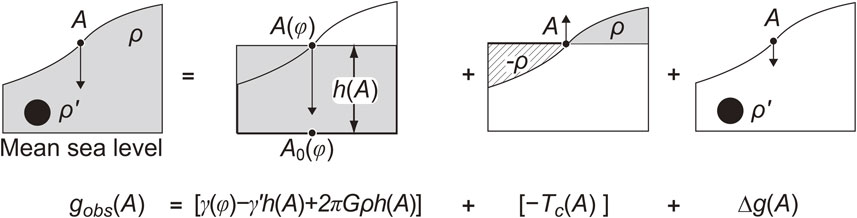
The gravity anomaly Δg. Terrestrial gravity g_obs at point A on the surface is decomposed into (1) γ, the normal gravity at the mean sea level A₀ at latitude φ, (2) −γ′h, the normal gravity difference between A and A₀, (3) 2πGρh, the attraction of an infinitely large flat plate of thickness h with density ρ, (4) −T_c, the topographic correction, and (5) Δg, the attraction of a subsurface body with an anomalous density. Note that we may always take both γ′ and T_c(A) to be positive because we consider downward to be the positive direction for terrestrial gravity.

The local gravity anomalies around volcanoes and seismic faults are usually within ±100 mGal or 10⁻⁴g₀. Based on various features of a gravity anomaly map, such as the one compiled by Shichi (2019)¹⁵⁾ (Fig. 2a), the geometries and density contrasts of the subsurface bodies can be estimated. For example, the very steep horizontal gravity gradient running from the Awaji Island to Kobe (Fig. 2b) strongly suggests the existence of a subsurface fault with a large density contrast in the NW–SE direction. Kobayashi et al. (1996)¹⁶⁾ quantitatively analyzed the gravity anomaly to determine the density structure using two-dimensional (2D) forward modeling.¹⁷⁾ Their results (Figs. 2c and 2d) clarify the subsurface fault between the Rokko granite and Osaka formation, which most probably slipped during the 1995 Kobe earthquake, leading to a death toll of more than 6000.

Fig. 2.

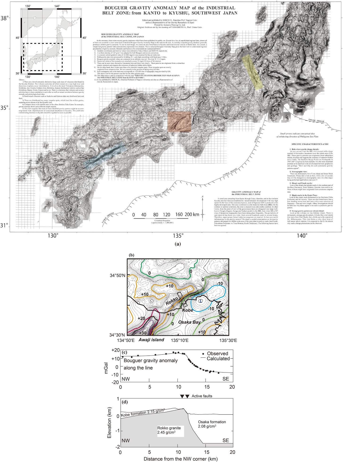
(a) Gravity anomalies in the southwest to central parts of Japan. Contour lines are drawn every 1 mGal. Steep horizontal gradient zones are clearly observable along the Median Tectonic Line (blue), the Itoigawa–Shizuoka Tectonic Line (yellow), and the fault zone of the 1995 Kobe earthquake (red). Redrawing of the original figure after Shichi (2019).¹⁵⁾

(b) Gravity anomalies around Kobe, where the M7 Kobe earthquake resulted in more than 6000 fatalities. The units are mGal, and the contours are drawn every 1 mGal. (c) Projection of the gravity anomalies along the rectangle in Fig. 2b around Kobe. (d) Subsurface density model beneath the rectangle in Fig. 2b derived from the gravity anomalies.

2.2. Nonuniqueness of gravimetric inversion for subsurface density.

The gravity analysis explained in section 2.1 is based on forward modeling. In this approach, a density model consistent with the observed gravity anomalies is searched for while considering the geophysical and geological constraints. However, the derived density model is not unique because there are numerous models that explain the gravity anomalies equally well. A trivial example is that the constant gravity g₀ on a sphere of radius a can be explained by a uniform sphere or a uniform spherical shell if they have the same mass M = g₀a²/G. Thus, the gravity data impose important constraints on the subsurface density distribution but the density structure estimated based on gravity anomalies alone is not free from the ambiguity inherent in any potential field such as the geomagnetic field.^18),19) To meaningfully interpret the gravity anomalies, additional geophysical information derived from seismic and geomagnetic/electric explorations as well as geological constraints is often necessary. The simultaneous inversion of gravity anomalies and seismic data is the most commonly used approach. However, it is not entirely free from ambiguities because it is necessary to assume an ad hoc relationship between the density and seismic P- and S-wave velocities. To circumvent this difficulty, we need observables other than gravity that are primarily sensitive to density. One of the candidates is the cosmic-ray flux penetrating a rock body. In the following section, we briefly describe the principle of cosmic-ray imaging and show how it can be integrated with gravity observations for three-dimensional (3D) density imaging.

2.3. Cosmic-ray radiography and its integrated analysis with gravity anomalies.

The first cosmic-ray muon image of the inside of a volcano was acquired in a pioneering study by Tanaka et al. (2007).²⁰⁾ Tanaka and Yokoyama (2008)²¹⁾ named the imaging technique muon radiography and applied it to probe the inside of Showa-shinzan volcano located in Hokkaido, Japan. In this approach, the absorption of cosmic-ray muons, as they penetrate rocks on their paths to a sensor on the ground, is measured (Fig. 3). The attenuation of the muon flux is governed by the density length X, defined as   

\begin{equation} X(\theta,\lambda) \equiv \int_{T} \rho (l, \theta, \lambda) dl = \bar{\rho} (\theta, \lambda) \cdot L (\theta,\lambda), \end{equation} [3]

  

\begin{equation} L (\theta,\lambda) = \int_{T} dl, \end{equation} [4]

  

\begin{equation} \bar{\rho} (\theta, \lambda) = X(\theta,\lambda)/L (\theta,\lambda), \end{equation} [5]

where ρ is the material density at a distance l from the sensor, θ and λ are the zenith angle and azimuth, respectively, of the incident muon; L is the path length within the target T, and $\bar{\rho }$ is the rock density averaged along the incident path (Fig. 3). Note that the path length L(θ, λ) in Eq. [4] can be accurately estimated when a digital elevation model is available. It follows that the pattern of the mean density $\bar{\rho }(\theta ,\lambda )$ can be easily derived from Eq. [5] once the density length X(θ, λ) is obtained from muon flux observations.²²⁾

Fig. 3.

Principle of cosmic-ray radiography. The figure shows a profile with a specific azimuth λ₀. The flux of muons reaching the ground sensor from the zenith angle θ and azimuth λ₀, N_rec, depends on the density ρ and the travel distance L along the path in the target. We may compute the density length X by comparing N_rec with the known incidence flux N_in.

The image of the muon radiographic density $\bar{\rho }(\theta ,\lambda )$ of a target can be compared to an X-ray snapshot. We should note here that a cosmic-ray image acquired by a sensor on the ground is a 2D section image averaged along the cosmic-ray paths to the sensor rather than a 3D density image. A simulation study showed that at least 16 2D muon radiographic images captured from independent directions are necessary to reconstruct a 3D density model of a target with a reasonable resolution.²³⁾ However, it is not practical to evenly distribute many muon detectors around a volcano having a rugged topography. Because long-term electric power supply is not feasible for such conditions, there is no alternative but to use the emulsion plates as muon detectors. However, in general, with an increasing number of muon detectors on the ground, more time is needed to scan and process the muon trajectories on the emulsion plates. An easier 3D density reconstruction method was expected, and Nishiyama et al. (2014)²⁴⁾ presented a breakthrough with respect to this problem, noting that both muon absorption and gravity are sensitive to the internal density structure. Specifically, they proposed the simultaneous inversion of the 2D muon radiographic data and gravity anomalies to obtain the 3D density structure (Fig. 4). They began by dividing a target volcano into N voxels with density ρ_j (j = 1,2,…, N). The gravity anomaly at the i-th gravity station on the ground at (x_i, y_i, z_i) can be expressed as   

\begin{equation} \Delta g_{i} \equiv \Delta g(x_{i},y_{i},z_{i}) = \sum_{j = 1}^{N}G_{ij}\rho_{j};\ i = 1,2, \ldots ,N_{G} \end{equation} [6]

where G_ij is the vertical component of gravity due to the j-th voxel with unit density at (x_j, y_j, z_j):   

\begin{equation} G_{ij} = G\iiint \frac{(z_{i} - z_{j})}{\left(\sqrt{(x_{i} - x_{j})^{2} + (y_{i} - y_{j})^{2} + (z_{i} - z_{j})^{2}}\right)^{3}}dV. \end{equation} [7]

On the other hand, the density length derived in the direction of the zenith angle θ_k and azimuth λ_k is related to the voxel density ρ_j as   

\begin{equation} X_{k} = \sum_{j = 1}^{N}L_{kj}\rho_{j};\ k = 1,2, \ldots,N_{C}, \end{equation} [8]

where L_kj is the length of the k-th trajectory passing through the j-th voxel (Fig. 4). Because Eqs. [6]–[8] show that the gravity and density length data are linearly related to the voxel density, they can be rewritten using the matrix $\tilde{\text{A}}$ and vectors $\vec{d}$ and $\vec{\rho }$ as   

\begin{equation} \vec{d} = \tilde{\text{A}}\vec{\rho}, \end{equation} [9]

  

\begin{align} \vec{d} &= (\Delta g_{1},\Delta g_{2}, \ldots,\Delta g_{N_{G}},X_{1,}X_{2,}, \ldots,X_{N_{C},})^{t},\\ \tilde{A} &= (\tilde{G},\tilde{L})^{t},\ \vec{\rho} = (\rho_{1},\rho_{1}, \ldots,\rho_{N})^{t}. \end{align} [10]

Fig. 4.

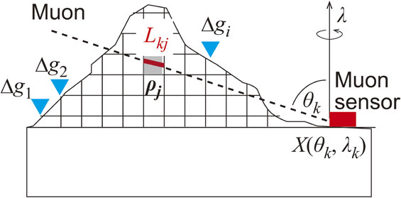
Principle of 3D density modeling by integrating the cosmic-ray radiography and gravity anomaly analysis. The density of each voxel is determined such that it simultaneously satisfies the muon flux and gravity anomalies. The flux of muons X(θ_k, λ_k) coming from the zenith angle θ_k and azimuth λ_k is dependent on the density ρ_j and travel distance L_kj along the path in the j-th voxel. The contribution of the j-th voxel to Δg_i, the gravity anomaly at the i-th point, is G_ij in Eq. [6].

Solving Eq. [9] for the voxel density $\vec{\rho }$ is a linear inverse problem. Nishiyama et al. (2016)²⁵⁾ applied this method to Showa-shinzan lava dome, Hokkaido, Japan and imaged its interior with unprecedented high resolutions of 0.1 and 0.2 km in the vertical and horizontal directions, respectively (Fig. 5). The resulting 3D image exhibits remarkable improvement when compared with the 2D section image.²¹⁾ It clearly shows a cylindrical column of massive matter with a diameter of 300 m oriented vertically, rising to the top of the lava dome (Fig. 5). This technique is widely applied to study the interiors of volcanoes worldwide such as La Soufrière de Guadeloupe.²⁶⁾

Fig. 5.

Showa-shinzan lava dome (left, courtesy of Dr. Ryuichi Nishiyama) and 3D representation of the density model (right) derived from the integrated analysis of the gravimetry and muon radiography, redrawing Fig. 6 of Nishiyama et al. (2016).²⁵⁾ The gravity points are shown using red solid squares, whereas the muon trajectories are drawn using blue lines.

3. Temporal gravity changes due to earthquakes

From the geophysical point of view, most earthquakes can be reasonably modeled in terms of a dislocation embedded in an elastic medium. Consequently, we can formulate the gravity changes as well as crustal deformations (i.e., displacements, tilt, and strains of the ground) in the framework of the dislocation theory.^27),28) In the following subsections, we will provide an overview of the theoretical and observational results with respect to the gravity changes for several important cases.

3.1. Gravity changes excited by a large earthquake when magnitude M < 8.

The terrestrial gravity field changes when a large earthquake occurs partly because the slip motion on the fault causes compression/dilation of the rocks around the fault and partly because the observation points are raised/lowered in space. The former necessarily causes a density change based on whether the rocks are compressed or dilated. The latter is the result of measuring the gravity at different points in space before and after an earthquake, provided that they are fixed on the deformable ground surface. Considering these two factors, Okubo (1992)²⁹⁾ derived formulas for the gravity and potential changes (Δg and ΔΨ, respectively) due to faulting on a finite rectangular plane in a homogeneous half-space (Fig. 6). These equations are useful for estimating Δg when the curvature of the Earth and the inhomogeneity of physical constants can be reasonably ignored. This is the case for large earthquakes having moment magnitudes of less than 8 because their fault dimensions are usually several tens of kilometers or less. Using the Cartesian coordinates (x₁, x₂, x₃), Δg at a point (x₁, x₂, x₃ = 0) fixed on the ground can be expressed as   

\begin{align} &\Delta g (x_{1}, x_{2}) \\ &\quad = \{\rho G [U_{1}S_{g} (\xi, \eta) + U_{2}D_{g} (\xi, \eta) + U_{3} T_{g} (\xi, \eta )]\\ &\qquad + (\rho' - \rho )GU_{3}C_{g} (\xi, \eta)\}{\parallel}-\beta\Delta h (x_{1}, x_{2}), \end{align} [11]

  

\begin{align} &\Delta \mathit{h} (x_{1}, x_{2}) \\ &\quad= [U_{1}S_{h} (\xi, \eta) + U_{2}D_{h} (\xi, \eta) + U_{3}T_{h} (\xi, \eta)]{\parallel}, \end{align} [12]

where U₁ and U₂ are the strike-slip and dip-slip components of fault motion during an earthquake, respectively; U₃ is the component perpendicular to the fault, which usually vanishes for ordinary earthquakes but is not equal to 0 when magma or hydrothermal water intrudes along a thin sheet to form a tensile opening (i.e., a dike or sill); ρ and ρ′ are the densities of the half-space and intruding matter, respectively; Δh and β ∼ 0.3086 (mGal/m) denote the uplift of the ground and the vertical gradient of the terrestrial gravity field, respectively. The symbol ∥ is defined by Chinnery (1961)³⁰⁾ as   

\begin{align} f(\xi, \eta){\parallel} &\equiv f (x_{1}, p) - f (x_{1}, p - W) \\ &\quad - f (x_{1} - L, p) + f (x_{1} - L, p - W), \end{align} [13]

  

\begin{equation} p \equiv x_{2} \cos \delta + d \sin \delta, \end{equation} [14]

where L, W, and δ are the length, width, and dip angle of the fault, respectively (Fig. 6); S_g, D_g, T_g, and C_g denote the contributions of strike-slip, dip-slip, tensile opening, and filling of the cavity sheet, respectively, and are given by Okubo (1992)²⁹⁾ in an analytical form; and S_h, D_h, and T_h are the contributions of strike-slip, dip-slip, and tensile opening to the uplift, respectively, as given by Okada (1985).²⁷⁾

Fig. 6.

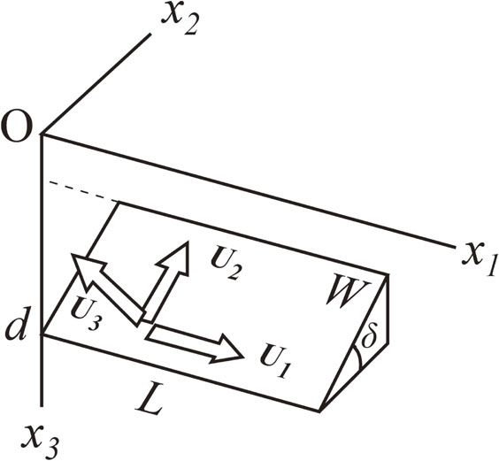
A rectangular fault of length L and width W embedded in a homogeneous half-space with a dip angle of δ. U₁, U₂, and U₃ denote the strike-slip, dip-slip, and tensile opening components, respectively.

The theoretical coseismic gravity change was observationally tested by Tanaka et al. (2001)¹²⁾ against the gravity changes observed during the Shizukuishi earthquake on September 3, 1998 (M6.1) by fulfilling all the technical requirements to verify the theory. They showed that the observed spatiotemporal gravity variations agreed remarkably well with those expected from Eqs. [11]–[14] when the fault parameters were estimated from the displacement data alone without using the gravity changes (Fig. 7). This was the first unequivocal detection of coseismic gravity changes and confirmed the validity of the theory. Currently, these expressions have been implemented in an earthquake simulator in California.³¹⁾

Fig. 7.

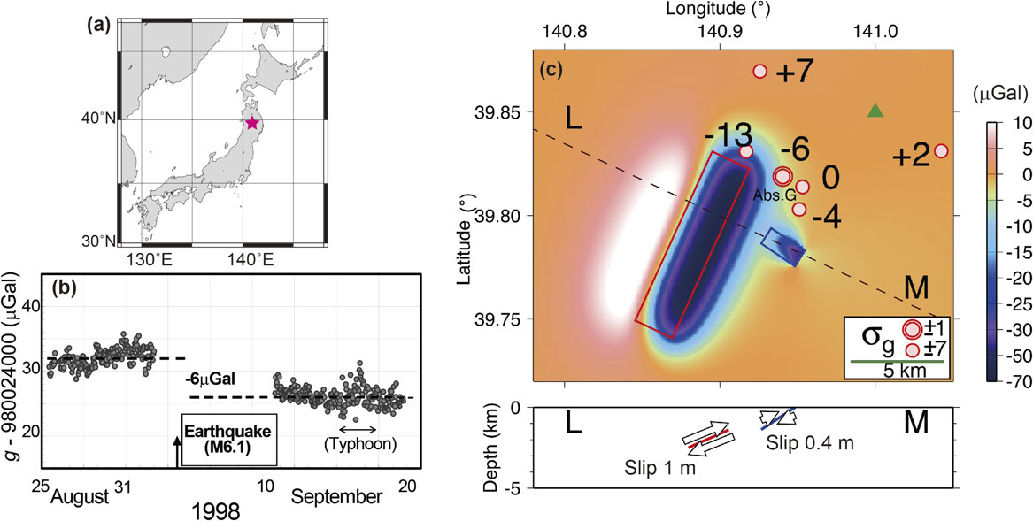
Gravity changes during the Shizukuishi earthquake (redrawing of the original figures from Tanaka et al. (2001)¹²⁾). (a) Epicenter is denoted using a red star. (b) Absolute gravity change during the earthquake. The measurement error is approximately 1–2 µGal. (c) (Top) Theoretical gravity changes (colors) and observed gravity changes (figures) during the M6.1 earthquake (the units are µGal), where σ_g denotes the measurement error. The blue and red rectangles are the faults projected on the surface. (Bottom) Cross-section along L–M viewed from the southwest. The slips on the larger and smaller faults are 1 and 0.4 m, respectively.

3.2. Gravity changes excited by a great earthquake (M > 8).

Estimation of the regional- to global-scale gravity changes excited by a great earthquake requires the consideration of the curvature and radial inhomogeneity of the Earth³²⁾ because they have unusually large fault areas covering several thousand square kilometers.³³⁾ For example, the fault length L and width W of the 2011 Tohoku earthquake were 500 and 200 km, respectively.^34),35) A fault length greater than 100 km implies that significant displacement and gravity changes are imposed beyond the epicentral distance of a few hundred kilometers and that the Earth can no longer be approximated to be flat. In addition, the density and elastic moduli vary significantly with depth along a fault because it penetrates the boundary between the crust and mantle located at a depth of 10–30 km.

Sun and Okubo (1993)³⁶⁾ was the first who succeeded in obtaining the theoretical coseismic gravity changes for a spherically symmetric, nonrotating, perfectly elastic, and isotropic (SNREI) Earth with self-gravitation. They presented a set of Green’s functions {G_ij(D_s, θ, λ); i, j = 1, 2, 3} describing the global gravity changes due to the dislocations of a unit seismic moment located on the polar axis (Fig. 8). Once the set of Green’s functions {G_ij; i, j = 1, 2, 3} has been computed, the gravity change Δg due to an earthquake can be easily estimated through numerical integration over the fault surface S as follows:³⁷⁾   

\begin{equation} \Delta g(\theta, \lambda) = \iint\nolimits_{s}G_{ij}(D_{s},\Theta,\Lambda)[\mu\ u_{i}\ n_{j}](\theta',\lambda')dS(\theta',\lambda'), \end{equation} [15]

where (θ, λ) denotes the colatitude and longitude of the observation point; D_s and (θ′, λ′) denote the depth, colatitude, and longitude of the infinitesimal fault dS in the integral, respectively; u_i and n_j denote the Cartesian components of the dislocation and a vector normal to the fault, respectively; and μ denotes the rigidity. In addition, Θ and Λ are the epicentral distance (as an angle) and azimuth of the observation point measured from the source given by the following spherical trigonometric relations:   

\begin{equation} \cos\Theta = \cos\theta\cos\theta' + \sin\theta\sin\theta'\cos(\lambda' - \lambda), \end{equation} [16]

  

\begin{equation} \sin\Theta\sin\Lambda = \sin\theta'\sin(\lambda - \lambda'), \end{equation} [17]

  

\begin{equation} \sin\Theta\cos\Lambda \sin\theta' = \cos\theta - \cos\theta'\cos\Theta. \end{equation} [18]

Fig. 8.

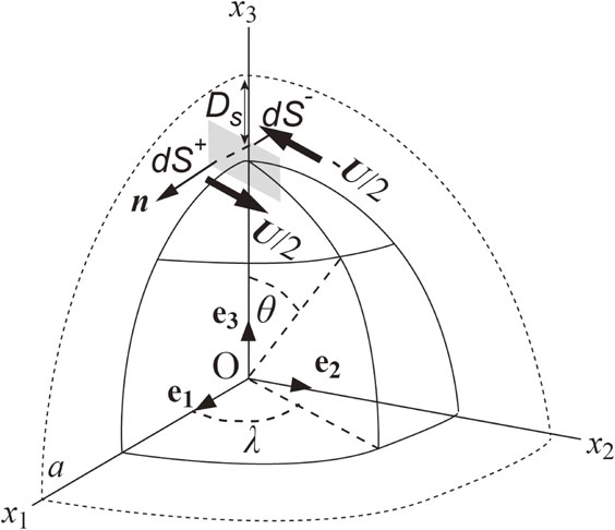
Point dislocation on the polar axis for the SNREI Earth. The dislocation vector U is assumed on an infinitely small rectangle defined by a normal vector n and area dS ≪ 1. D_s and a denote the source depth and the Earth’s radius, respectively.

It took ten years for the theory of Sun and Okubo to be verified by the observations of Imanishi et al. (2004),³⁸⁾ who detected the regional gravity changes during the 2003 Tokachi-oki earthquake (M8.0) using an array of superconducting gravimeters (SGs) (Fig. 9). In a series of studies, the author’s research group predicted that great earthquakes cause gravity changes on regional to global scales exceeding the signal level of modern satellite gravity missions.^39)–41) In fact, the GRACE (Gravity Recovery and Climate Experiment) satellite mission⁴²⁾ detected significant gravity changes during the 2004 Indian Ocean earthquake off the coast of Sumatra, Indonesia (M9.1), the 2010 Maule earthquake in central Chile (M8.8), and the 2011 Tohoku earthquake in Japan (M9.1) consistent with the theoretical expectations according to Eq. [15].^43)–45)

Fig. 9.

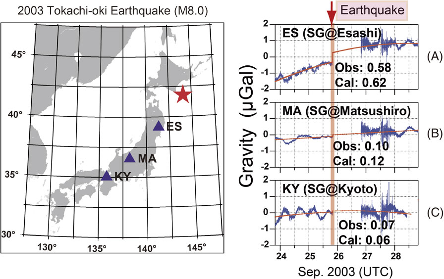
Regional gravity changes detected with an array of SGs (redrawing of the original figures from Imanishi et al. (2004)³⁸⁾). The units are µGal. (Left) Epicenter (a red star) of the 2003 Tokachi-oki earthquake and the SG station locations (triangles). ES, Esashi; MA, Matsushiro; KY, Kyoto. (Right) Gravity data (blue) recorded by SGs for the Tokachi-oki earthquake in 2003. The units are µGal. (A) Esashi, (B) Matsushiro, and (C) Kyoto. The red curves are the smoothed values obtained by considering the coseismic gravity steps and instrumental long-term drift.

4. Temporal gravity changes due to volcanic activity

4.1. Physical modeling of volcanic eruptions.

A volcanic eruption can be defined as the ejection of liquid or solid matter, such as lava and tephra, from the ground through vents. The most familiar type of eruption is summit eruption, in which a crater located around the center of the edifice serves as the vent. If an eruption occurs on the sides located at a considerable distance from the summit, it may be called a flank eruption. The other important type of eruption is a fissure eruption, in which magmatic matter is ejected from the vents along a line on the ground extending for many kilometers. Fissure eruptions are often found at places where the tensile tectonic stress is dominant, as in rift valleys and mid-oceanic ridges.

Physical models of these eruptions usually comprise several components: (1) an inflating or deflating magma chamber located at a depth of 1 to 10 km, (2) a conduit, serving as a pathway for the magma from the chamber to the surface, and (3) a dike connecting the magma chamber to linear fissures on the ground. In the following subsections, we will integrate these components to discuss the gravity changes and crustal deformations from the theoretical and observational perspectives.

4.2. Summit/flank eruption — modeling with a blocked conduit coupled to a magma chamber.

The volcano deformation preceding a summit or flank eruption can be modeled by assuming a coupled magma chamber and conduit. As the conduit is usually blocked or plugged with solidified magma until the moment of eruption, the overpressure ΔP builds up effectively in the magma chamber when magma is fed from below or volcanic gases exsolve from the melt in the chamber. As a first approximation, the crustal deformation can be analyzed using the Mogi model.⁴⁶⁾ It assumes a spherical pressurized source embedded in a homogeneous elastic half-space, ignoring the conduit deformation. If the source radius a is considerably less than the source depth D, the elastic displacements (u_r, u_θ, u_z) on the surface are given by Yamakawa (1955)⁴⁷⁾ as   

\begin{equation} \vec{u} = (u_{r},u_{\theta},u_{z}) = \frac{(1 - \nu)\Delta P}{\mu} \frac{a^{3}}{(r^{2} + D^{2})^{\frac{3}{2}}}\quad (r,0,D), \end{equation} [19]

where r, θ, and z are the conventional cylindrical coordinates, with the origin located on the ground just above the pressure source, and μ and ν are the rigidity and Poisson’s ratio of the medium, respectively. Equation [19] can be rewritten in terms of ΔV, the volume change of the inflating magma reservoir, as   

\begin{equation} (u_{r},u_{\theta},u_{z}) = \frac{(1 - \nu)}{\pi}\frac{\Delta V}{(r^{2} + D^{2})^{\frac{3}{2}}}\quad (r,0,D). \end{equation} [20]

The observables, such as the radial tilt t and radial strain ε on the surface, can be derived as   

\begin{equation} t = -\frac{\partial u_{z}}{\partial r},\quad \varepsilon = \frac{\partial u_{r}}{\partial r}. \end{equation} [21]

The surface gravity change Δg measured at a fixed point on the ground comprises the following four contributions: (1) the free-air gravity change due to the uplift of the observation point u_z; (2) the attraction of the surface mass distribution (single layer) originating from the deformed ground having density ρ and thickness u_z; (3) the attraction from the perturbed density field ($ - \rho \,\text{div}\,\vec{u})$ within the Earth; and (4) the direct attraction of the mass transported to/from the magma reservoir ΔM. Hagiwara (1977)⁴⁸⁾ provided analytical solutions for each aforementioned contribution. The resulting total gravity change on the surface can be expressed as   

\begin{equation} \Delta g(r) = -\beta u_{z}(r) + G\Delta M\frac{D}{(r^{2} + D^{2})^{\frac{3}{2}}}, \end{equation} [22]

where β = 0.3086 mGal/m implies the free-air gravity gradient; ΔM is the mass transported to the magma chamber during the inflation process and is related to the uplift u_z from Eq. [20] according to   

\begin{equation} \Delta M = \rho_{0}\Delta V = \rho_{0}\left(\frac{\pi}{1 - \nu}\right)\frac{(r^{2} + D^{2})^{\frac{3}{2}}}{D}u_{z}(r), \end{equation} [23]

where ρ₀ is the density of the matter involved in the inflation process. By substituting Eq. [23] into [22], we obtain   

\begin{equation} \Delta g(r) = \left(- \beta + \frac{\rho_{0}\pi G}{1 - \nu}\right)u_{z}(r). \end{equation} [24]

If bubble formation of volatile gases in the magma chamber is responsible for the inflation, the ratio of the gravity change to uplift yields   

\begin{equation} \frac{\Delta g(r)}{u_{z}(r)} \sim -\beta = -0.31\,\text{mGal/m} \end{equation} [25]

because $\rho _{0} \ll \frac{\beta }{G}$. On the other hand, if the inflation originates from the supply of melt from a deeper part, we obtain   

\begin{equation} \frac{\Delta g(r)}{u_{z}(r)} = -0.23\,\text{mGal/m} \end{equation} [26]

by assuming ρ₀ = 3 × 10³ kg/m³ and ν = 1/4. Equations [24]–[26] clearly show that the ratio $\frac{\Delta g}{u_{z}}$ is independent of the distance from the inflation source and provides invaluable information regarding ρ₀, i.e., the density of the transported matter. It should be emphasized that ρ₀ is never obtained by analyzing displacement data alone, as can be seen in Eq. [19]. It is only recoverable from the simultaneous observations of the gravity and elevation changes.

After the volcanic mass (lava, tephra, and gases) is ejected from a summit or flank crater during an eruption, the overpressure ΔP is lowered and the volcano usually undergoes deflation. Although the conduit is no longer blocked, Eqs. [19]–[23] still provide an appropriate model for computing the deformation and gravity changes during the eruption by considering negative values of ΔP and ΔV to model the deflating magma chamber. This formulation will be used to analyze the gravity change for a deflating pressure source in section 4.5.

4.3. Continual summit/flank eruption — modeling with an open conduit coupled to a magma chamber.

Volcanic eruptions often occur continually from the same crater for periods ranging from a month to years, as was the case for the volcanic activities of Asama volcano, Honshu, Japan in 2004 and Sakura-jima volcano from 2009 to 2016. Continual Vulcanian explosions from the same crater strongly suggest that the conduit is mostly open, implying that the overpressure inside the magma chamber is continually released at the surface. This results in only minor crustal deformation but the gravity changes can still be as large as those in the cases of blocked conduits, as can be observed below.

Let us now consider magma rising in a conduit open at the top. As a first approximation, we may assume a vertical open pipe of radius a_pipe linked to a pressurized sphere of radius a_sph embedded at depth D_sph in an elastic half-space of rigidity μ (Fig. 10).⁴⁹⁾ The pipe represents the conduit, whereas the sphere corresponds to the magma chamber. We assume that the pipe is initially filled with magma up to an elevation of H_head. When magma of density ρ is supplied to the system from below by volume ΔV_inflow, a uniform pressure change ΔP is expected in the sphere and most of the pipe. In the newly filled portion of the pipe, the pressure linearly decreases with the elevation. Ignoring the compressibility of the magma, we obtain   

\begin{equation} \Delta V_{\textit{inflow}} = \Delta V_{\textit{head}} + \Delta V_{\textit{pipe}} + \Delta V_{\textit{sph}} \end{equation} [27]

from the law of mass conservation, where ΔV_head is the volume of the ascending column and ΔV_pipe and ΔV_sph are the volume changes of the pipe and the sphere, respectively (Fig. 10). Specifically,   

\begin{equation} \Delta V_{\textit{head}} = \pi a_{\textit{pipe}}^{2}\Delta H_{\textit{head}}, \end{equation} [28]

  

\begin{equation} \Delta V_{\textit{pipe}} = 2\pi a_{\textit{pipe}}\Delta a_{\textit{pipe}}(D_{\textit{sph}} + H_{\textit{head}}), \end{equation} [29]

  

\begin{equation} \Delta V_{\textit{sph}} = 4\pi a_{\textit{sph}}^{2}\Delta a_{\textit{sph}}, \end{equation} [30]

where ΔH_head is the elevation change of magma head given by $\Delta H_{head} = \frac{\Delta P}{\rho g}$ using g = 9.8 m/s² as the standard gravity on the Earth’s surface. Because the radial expansions of the pipe and sphere are given by Bonaccorso and Davis (1999)⁵⁰⁾ and Yamakawa (1955)⁴⁷⁾ as   

\begin{equation} \Delta a_{\textit{pipe}} = \frac{a_{\textit{pipe}}\Delta P}{\mu},\ \Delta a_{\textit{sph}} = \frac{a_{\textit{sph}}\Delta P}{4\mu}, \end{equation} [31]

we obtain   

\begin{equation} \frac{\Delta V_{\textit{head}}}{\Delta V_{\textit{inflow}}} = 0.946,\ \frac{\Delta V_{\textit{pipe}}}{\Delta V_{\textit{inflow}}} = 0.016,\ \frac{\Delta V_{\textit{sph}}}{\Delta V_{\textit{inflow}}} = 0.038 \end{equation} [32]

by assuming reasonable values of a_pipe = 70 m, a_sph = 500 m, D_sph = 5000 m, H_head = 400 m, and (μ/ρ)$^{\frac{1}{2}}$ = 2500 m/s. It is obvious from Eq. [32] that most of the supplied mass is used to raise the magma head. It follows that the gravity change for the open conduit system is primarily governed by the direct attraction from the raised mass in the conduit.

Fig. 10.

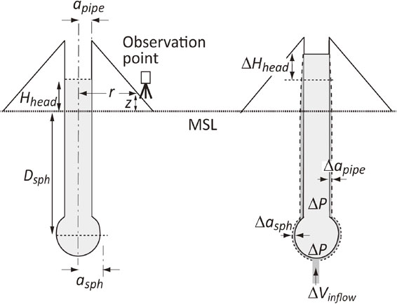
An open conduit coupled to a magma chamber modeled as a cylindrical pipe linked to a spherical pressure source. (Left) Reference state. (Right) When magma is supplied to the magma chamber, the resulting excess pressure causes elastic deformation of the pipe and sphere along with the rising magma head.

The continual summit eruptions of Asama volcano in 2004 can be successfully explained using the open conduit coupled to a magma chamber (Figs. 11a and 11b). The conduit is likely to have been opened to the free surface by the first Vulcanian eruption on September 1, 2004, which blew off the plug at the top of the conduit. Subsequent volcanic events, such as the formation of a lava cake around the vent, indicate that the conduit remained open at least throughout September 2004 (Table 1). It follows that the terrestrial gravity should vary as the magma head rises and falls in an open conduit during this period. Figure 11c shows the gravity change Δg(t) measured at 4 km from the summit since September 8, 2004. The point of greatest interest is that eruptions have always occurred when Δg(t) was decreasing to a local minimum. A simple explanation of this correlation is provided in Fig. 11d. As the magma head rises above the observation point toward the vent, the magma in the conduit attracts the gravimeter upward, partially eliminating the downward terrestrial gravity and resulting in a gravity decrease.

Fig. 11.

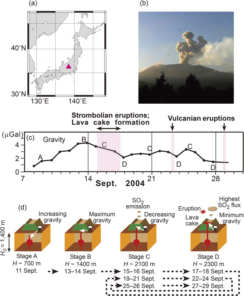
(a) Location of Asama volcano, denoted by a red triangle. (b) Eruption on September 15, 2004, 17:19 JST (courtesy of Dr. Mitsuhiro Yoshimoto). (c) Gravity variations (minus the nominal value of 979 869 900 µGal) measured at the Asama Volcano Observatory during September 2004. (d) Diagrams of the rise and fall of the magma head derived from the gravity data. The maximum gravity is observed when the magma head reaches the elevation of the gravimeter.

Table 1. Chronology of the volcanic unrest at Asama volcano in 2004 (based on Nakada et al. (2005)⁵¹⁾)

Date	Event description
July–August 2004	Gradual increase of the baseline length between two points across the summit, suggesting inflation of the edifice.
September 1, 2004	First Vulcanian eruption ejecting country rocks without magmatic matter, indicating that the plug at the top of the conduit was blown off.
September 15–17, 2004	Strombolian eruptions occurred continually. Lava cake was detected from a SAR (synthetic aperture radar) image on September 16, 2004.
September 23, 2004	Second Vulcanian eruption.
September 29, 2004	Third Vulcanian eruption.
October 1, 2004	Depression found in the central part of the lava cake, suggesting drain-back of the magma in the conduit.
October–December 2004	Vulcanian eruptions on October 10 and November 14, 2004.

Let us now quantitatively evaluate the gravity change. Because the radius of the conduit a ∼ 100 m is much smaller than the horizontal distance between the conduit and the observation point L = 4000 m, the attraction of magma Δg can be appropriately expressed using the following line mass model (Fig. 12a):   

\begin{align} \Delta g(H(t)) &= \pi G\rho_{\textit{melt}}a^{2}\phi\left(\frac{1}{\sqrt{L^{2} + (H(t) - H_{0})^{2}}} - \frac{1}{L}\right) \\ &\quad + \Delta g_{0}, \end{align} [33]

  

\begin{equation} \Delta g_{0} \equiv g(H(t) = H_{0}), \end{equation} [34]

where H(t) is the height of the magma head above the mean sea level (MSL) at time t, H₀ is the height of the gravity station above the MSL (Fig. 12b), and ρ_melt and ϕ denote the density of the magma and conduit porosity, respectively. By substituting appropriate values derived from the muon radiography,²²⁾ i.e., a = 110 m, ρ_melt = 2.67 g/cm³, and ϕ = 0.67, Eq. [33] can be solved for H(t) from the observed daily gravity change Δg(t) (Fig. 12b). It should be noted here that Eq. [33], which relates Δg to H, is not single-valued. This ambiguity can be resolved by noting that H(t) is a continuous function of time and by taking an appropriate initial condition. We take H = H₁ = 2500 m on September 18, 2004, when a 0.9 × 10⁶-m³ lava mound was formed on the summit crater of Asama volcano.

Fig. 12.

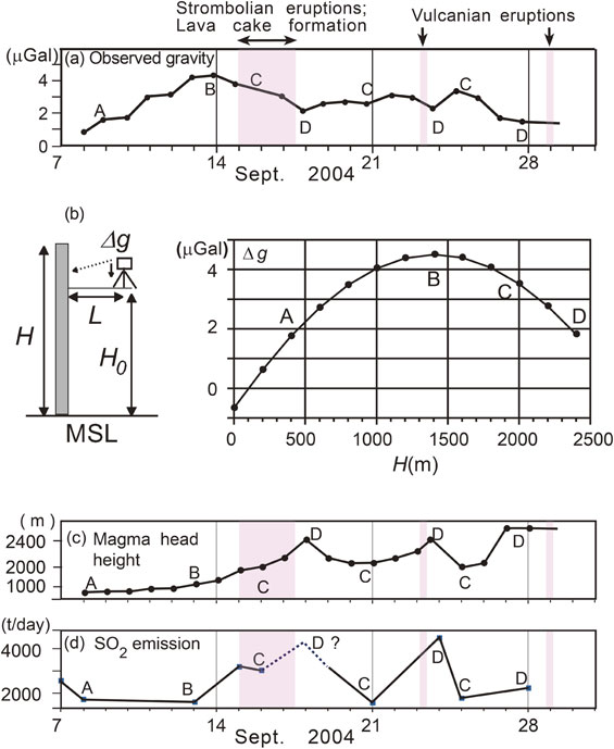
Modeling of the magma in a conduit. Labels A, B, C, and D correspond to magma head heights of 400, 1400 (observation site elevation), 2000, and 2400 m (summit elevation), respectively. (a) Gravity change. Same as Fig. 11c. (b) The line mass model used to calculate the magma head elevation. A gravimeter was installed at an elevation H₀ above the MSL. The distance from the conduit to the gravimeter is L. (c) The magma head height H derived from the gravity changes, as described in Eq. [33]. (d) The SO₂ emission rate measured with a compact UV spectrometer.⁵³⁾

The calculated magma head height H(t) reveals the rise of the magma to the top of the vent immediately preceding the three major eruptions (Fig. 12c). Two other observations support this result. The first is the SO₂ flux that was repeatedly measured using a compact UV spectrometer system.⁵²⁾ Compared with the emission rate of ∼100 t/day before the first eruption on September 1, 2004, an unusually high rate of several thousand t/day was observed during periods of continual Strombolian eruption (September 15–17, 2004) and the second Vulcanian eruption (September 23, 2004) (Fig. 12d).⁵³⁾ The active degassing during phases C–D can be well explained in our scenario (Fig. 11d) as a result of the lowered pressure at the magma/atmosphere interface when the magma head rose; SO₂ exsolves from magma only under pressures of less than 2–3 MPa or equivalent to 100–150 m lithostatic or shallower below the summit.⁵⁴⁾ This concept is supported by the fact that a lava dome with a volume of 0.9 × 10⁶ m³ appeared on the summit on September 16, 2004.⁵⁵⁾ Thus, the gravity analysis provides a tool for accurately estimating the magma head height.

4.4. Fissure eruption — modeling with dike/sill intrusion coupled to a magma chamber.

Recent fissure eruptions in Japan include the 1986 Izu-Oshima eruption,⁵⁶⁾ the submarine eruption off the coast of Ito in 1989,⁵⁷⁾ and the Miyake-jima eruption in 2000.⁵⁸⁾ They are characterized by crustal deformations with mirror symmetries on a line on which fissure vents are created. The symmetry is a result of elastic deformation when a thin vertical planar sheet of magma intrudes into country rock as a dike. When the dike reaches the surface, linear or echelon fissures are created on the ground, from which lava is ejected as a curtain of fire. It follows that the tensile dislocation model discussed in section 3.1 provides an adequate mathematical framework for describing the gravity changes during fissure eruption. Therefore, it is only necessary to assume the vanishing tangential dislocation, U₁ = U₂ = 0, in Eqs. [11] and [12]. It should be noted here that the intrusions require mass transport from a deeper source, most likely from a magma reservoir. Consequently, dike intrusion is expected to be accompanied by magma chamber deflation. The model of a dike coupled to a magma chamber will be used in section 4.5 to analyze the gravity changes during the eruption of Miyake-jima volcano in 2000.

4.5. Hybrid gravity observation during caldera formation.

A caldera is the depressed topography often found on top of a volcano. Most calderas are believed to have been formed by the collapse of the tops of volcanic cones into the space formed by an ejection or by the lateral outflow of magma during volcanic eruptions.⁵⁹⁾ However, details of the formation process are not yet well understood among volcanologists,⁶⁰⁾ primarily because such events have rarely been witnessed.⁶¹⁾ The Miyake-jima volcanic eruption in 2000 provided a rare opportunity to study the process of caldera formation using modern observation instruments. Table 2 summarizes how the volcanic activity evolved during the first two months, following the onset of volcanic unrest.

Table 2. Chronology of the volcanic unrest at Miyake-jima Island in 2000

Date	Event description
June 26, 2000	Onset of an earthquake swarm below Miyake-jima volcano. A significant ground tilt of ∼0.1 mrad indicated swelling of the volcano due to dike intrusion with the E–W strike.62)
June 27, 2000	Submarine fissure eruption off the west coast of the island with the E–W strike.
June 27–July 1, 2000	Migration of the hypocenters from the west coast toward the northwest for more than 20 km, strongly suggesting the lateral dike intrusion of magma from Miyake-jima.
June 28–July 7, 2000	Gradual subsidence of the ground revealed by the tilt and GPS observations.
July 4–mid-August 2000	A remarkable increase in seismicity just below the summit; hypocenters were mostly confined to a cylindrical volume of 500-m radius extending to 2500 m below the sea level.63)
July 8, 2000	A small summit eruption lasting for 10 min.
July 9, 2000	A pit crater of ∼800-m diameter and 100–200-m depth was found on the top, most likely due to the collapse of the summit into the cavity.64)
July 10–September 30, 2000	Growth of the crater to form a caldera of 1.6 km diameter and 500-m depth.63)

Modern hybrid gravity measurements were performed on Miyake-jima volcano to reveal the gravity changes from June 1998 to July 6, 2000.^65),66) The results are intriguing because decreases in gravity by as much as 145 µGal were found in the summit area only two days before the collapse on July 8, 2000 (Fig. 13b). Further, a significant gravity increase of approximately 100 µGal was observed on the west coast, where fissures were found on the ground along the line of the offshore submarine eruption vents. The author’s research group postulated an integrated physical model comprising (1) a dike responsible for the fissure eruption on June 28, 2000 and the migrating earthquake swarm, (2) a deflating magma chamber linked to the dike, and (3) a cavity created by stoping beneath the summit when magma flowed out of the chamber. By assigning reasonable values to the parameters (Table 3, Fig. 13d), the three-element model reproduces the observed gravity change (Figs. 13b and 13c) and ground displacements detected by GPS.^65),66) Because the spherical cavity with a radius of ∼240 m (Table 3) is comparable in size to the fresh pit crater (∼800-m diameter) found on July 9, 2000 (Table 2, Fig. 13d), the significant gravity decrease in the summit area demonstrates the presence of a cavity before the collapse of the summit. The cavity is likely to serve as a seed for the growing caldera.

Fig. 13.

Volcanism of Miyake-jima in 2000. (a) Location of Miyake-jima volcano, indicated by a red triangle. (b) The observed gravity changes two days before the caldera collapse on July 8, 2000. The reference gravity was measured in June 1998. (c) The expected gravity changes based on the physical model given in Table 3. (d) Diagram of the physical model inferred based on the gravity and crustal deformation data. (e) Photo captured on July 9, 2000 after the collapse of the summit (courtesy of Prof. Setsuya Nakada).

Table 3. A physical model to explain the gravity change and displacement of Miyake-jima from 1998 until July 6, 2000, two days prior to the collapse of the summit

Deflating sphere
Depth	5.3 ± 0.45 km
Volume change	−8.7 ± 0.5 × 107 m3
Density	2600 kg/m3
Spherical cavity
Depth	1.7 ± 0.2 km
Radius	240 ± 20 m
Density contrast	−2300 kg/m3
Rectangular dike
Strike direction	N60°W
Open dislocation	1.6 ± 1.0 m
Horizontal length	13.5 ± 1.0 km
Vertical width	10 km
Density of the intruding matter	2600 kg/m3

The pit crater continued to grow until the end of September 2000 to form a caldera of 1.6 km in diameter, indicating that a huge volume of 6 × 10⁸ m³, equivalent to a mass of 1 × 10⁹ t, must have been transported from Miyake-jima to somewhere else. In the following, we show that the absolute gravity data for Miyake-jima constrain mass movement during the caldera formation. We further decompose the gravity changes on Miyake-jima Island into three parts: (1) attraction associated with the lost mass around the caldera; (2) the Bouguer effect of the local uplift/subsidence on gravity; and (3) the residual (Fig. 14a). The first two components can be accurately estimated by using the topography change data⁶⁷⁾ and the GPS data⁶⁸⁾ during the period. We note that the residual gravity on Miyake-jima Island remained as small as ±2 µGal during the entire period. The destination of the transported mass is constrained by the condition that the downward attraction due to the migrated mass must be equal to the residual gravity within observational error. Figure 14b shows the Newton attraction expected at the gravity station of Miyake-jima as a function of the horizontal distance and depth of the destination. The areas marked in red in Fig. 14b, just below Miyake-jima volcano, are the most implausible destinations. Thus, we can reject the hypothesis that the magma drained back to deeper parts beneath the volcano during the collapse of the summit. The preferred destination is found in the area located 15–40 km from Miyake-jima, suggesting the lateral transport of the magma.

Fig. 14.

Search for the destination of the mass transported from Miyake-jima. (a) The gravity changes observed at the absolute gravity station on Miyake-jima volcano (blue) comprise the topographic change effect (green), the Bouguer effect of site elevation change (orange), and the remainder (red). (b) Newton attraction expected at the gravity station of Miyake-jima when a mass of 10⁹ t is transported to a spherical region centered at a specified depth and distance from Miyake-jima. The units of attraction are µGal.

The results are intriguing because an intensive earthquake swarm of more than 20000 microearthquakes occurred 15–35 km away from Miyake-jima volcano during the caldera formation period (Fig. 15c).⁶³⁾ It is likely that the transport of fluid magma triggered the microearthquakes partly because the effective confining pressure must be reduced by the intruding fluid. In addition, the significant displacements around the swarm area⁶⁹⁾ indicate a tensile opening of 6 m on a vertical plane that is 20 km in length and extends from 2 to 20 km in depth (Figs. 15d and 15e).⁶⁹⁾ The 2 × 10⁹-m³ space created by the tensile opening is comparable in volume to the 0.6 × 10⁹-m³ mass lost from Miyake-jima. Data pertaining to the gravity, hypocenters, and crustal displacement convinced us of the lateral magma flow from Miyake-jima and the resulting collapse of the volcanic edifice, i.e., caldera growth (Fig. 15b).

Fig. 15.

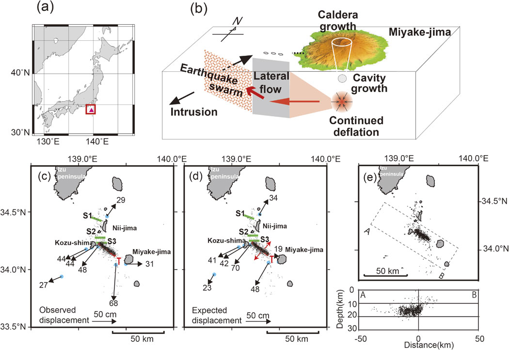
Magma movement from Miyake-jima volcano from July to September 2000.⁷⁰⁾ (a) The study area is indicated by the red square. The red triangle indicates Miyake-jima volcano. (b) A conceptual model that provides a comprehensive explanation of the growth of the Miyake-jima caldera, earthquake swarm, and crustal deformation. (c) Displacements as large as 20–60 cm are observed around the swarm area. The numerous small dots are epicenters of ∼20000 small earthquakes. S1, S2, and S3 denote the strike-slip faults responsible for M6 class earthquakes during the period. (d) Horizontal displacement expected for a tensile opening of 6 m on a vertical plane (20 km × 17 km) denoted by a red line “T” and three other supplementary strike-slips: 0.5 m on S1, 0.5 m on S2, and 1.5 m on S3. (e) Hypocenter distribution of the earthquakes with magnitudes greater than 3.5 from July 1 to September 30, 2000 after the unified seismic catalog of the Japan Metrological Agency. The hypocenters lie on a vertical plane at depths of 2–20 km.

5. Discussion and conclusions

Herein, we have provided an overview of the advances in gravity research on volcanic eruptions and earthquakes. Static investigations based on the gravity anomalies are still useful for detecting the possible faults of future earthquakes in Japan and other earthquake-prone areas. A more modern technique that integrates gravimetry and muon radiography is expected to flourish in the revelation of the volcanic interiors. With respect to the dynamic aspect, the author’s research group devised a theoretical framework for the gravity changes due to dislocations. The importance of this framework will increase further with respect to earthquake science because the hybrid gravity measurements and dedicated satellite gravity missions provide gravity data as accurate as 1 µGal more efficiently than that obtained previously. Integrated analysis using the two observational tools is considerably useful when studying the co- and postseismic processes within the Earth on a regional to global scale because they are complementary. The former has no limitations in terms of spatial resolution but is only applicable to the gravity changes on land, whereas the latter yields data over the sea even though its spatial resolution is limited to a few hundred kilometers.

It should be noted here that gravity analysis is limited by the disturbances caused by groundwater. Unusual gravity changes are often observed after heavy rainfall of >50 mm/day.⁷¹⁾ Consequently, the gravity method of studying earthquakes and volcanic activity does not work without appropriately correcting the gravity disturbances caused by groundwater. Kazama and Okubo (2009)⁷²⁾ provided a solution to this problem based on physical hydrology. The effectiveness of the hydrological correction method was proved in subsequent studies conducted by the author’s research group.^73)–75)

Because no physical observables other than gravity are sensitive to mass redistribution within the deep interior of the Earth, gravity analyses will continue to provide invaluable information about the transport of magma beneath volcanoes and the possible effects of fluids on the earthquake processes.^75)–77)

Acknowledgments

The author expresses his sincere thanks to the anonymous reviewers for their help in improving this manuscript. He is also deeply thankful to Prof. M. Amalvict for her explanation about Richer’s manuscript. Figure 15(e) was drawn using the Wellweb system of the Geological Survey Institute of Japan (https://gbank.gsj.jp/wellweb/cgi-bin/GSJ/earth/epicenter/res?0). This work was supported by the JSPS KAKENHI Grant Number 18H01305.

Notes

Edited by Yoshio FUKAO, M.J.A.

Correspondence should be addressed: S. Okubo, Earthquake Research Institute, The University of Tokyo, 7-3-1 Hongo, Bunkyo-ku, Tokyo 113-0033, Japan; Faculty of Geosciences and Environmental Engineering, Southwest Jiaotong University, West Park, Hitech Zone, Chengdu, Shichuan 611756, China (e-mail: [e-mail], [e-mail]).

References

• 1)  Richer, J. (1679) Observations Astronomiques et Physiques Faites en L’Isle de Caïenne. Mémoires de l’Academie Royale des Sciences, Paris. https://archive.org/details/bub_gb_uey3wMEY918C" target="_blank" rel="noopener noreferrer" class="bluelink-style">https://archive.org/details/bub_gb_uey3wMEY918C.
• 2)   Sakuma,  A. (1963) État actuel de la nouvelle détermination absolue de la pesanteur au Bureau International des Poids et Mésures, Sèvres. Bull. Geod. 69, 249–260.
• 3)  Faller, J.E. (1963) An absolute interferometric determination of the acceleration of gravity, Ph.D. Thesis, Princeton University.
• 4)   Niebauer,  T.M.,  Sasagawa,  G.,  Faller,  J.E.,  Hilt,  R. and  Klopping,  F.J. (1995) A new generation of absolute gravimeters. Metrologia 32, 159–180.
• 5)   Okubo,  S.,  Yoshida,  S.,  Sato,  T.,  Tamura,  Y. and  Imanishi,  Y. (1997) Verifying the precision of a new generation absolute gravimeter FG5 — Comparison with superconducting gravimeters and detection of oceanic loading tide. Geophys. Res. Lett. 24, 489–492.
• 6)  Torge, W. (1989) Gravimetry. de Gruyter, Berlin.
• 7)  Okubo, S., Satomura, M., Furuya, M., Sun, W., Matsumoto, S., Ueki, S. et al. (2002) Grand design for the hybrid gravity network around the Mt. Fuji volcano. In International Symposium on Geodesy in Kanazawa abstract, pp. 39–40.
• 8)  Hinderer, J., Hector, B., Mémin, A. and Calvo, M. (2016) Hybrid gravimetry as a tool to monitor surface and underground mass changes. In International Symposium on Earth and Environmental Sciences for Future Generations. International Association of Geodesy Symposia, Vol. 147 (eds. Freymueller, J.T. and Sánchez, L.). Springer, Cham, pp. 123–130.
• 9)   Yokoyama,  I. (1963) Structure of caldera and gravity anomaly. Bull. Volcanol. 26, 67–72.
• 10)   Fukao,  Y.,  Yamamoto,  A. and  Kono,  M. (1989) Gravity anomaly across the Peruvian Andes. J. Geophys. Res. 94, 3867–3890.
• 11)   Kono,  M.,  Fukao,  Y. and  Yamamoto,  A. (1989) Mountain building in the central Andes. J. Geophys. Res. 94, 3891–3905.
• 12)   Tanaka,  Y.,  Okubo,  S.,  Machida,  M.,  Kimura,  I. and  Kosuge,  T. (2001) First detection of absolute gravity change caused by earthquake. Geophys. Res. Lett. 28, 2979–2981.
• 13)   Furuya,  M.,  Okubo,  S.,  Sun,  W.,  Tanaka,  Y.,  Oikawa,  J.,  Watanabe,  H. (2003) Spatiotemporal gravity changes at Miyakejima Volcano, Japan: Caldera collapse. explosive eruptions and magma movement. J. Geophys. Res. 108, 2219.
• 14)  Hoffman-Wellenhof, B. and Moritz, H. (2005) Physical Geodesy. Springer, Wien.
• 15)   Shichi,  R. (2019) Bouguer gravity anomaly map of the industrial belt zone from Kanto to Kyushu, southwest Japan. Earthq. J. 67, 54–57 (in Japanese). https://www.static.jishin.go.jp/resource/figure/figure999009.jpg" target="_blank" rel="noopener noreferrer" class="bluelink-style">https://www.static.jishin.go.jp/resource/figure/figure999009.jpg.
• 16)   Kobayashi,  S.,  Yoshida,  S.,  Okubo,  S.,  Shichi,  R.,  Shimamoto,  T. and  Kato,  T. (1996) Two-dimensional analysis of gravity anomaly across the Rokko fault system. J. Phys. Earth 44, 357–372.
• 17)   Talwani,  M.,  Worzel,  J.L. and  Landisman,  M. (1959) Rapid gravity computations for two-dimensional bodies with application to the Mendocino submarine fracture zone. J. Geophys. Res. 64, 49–59.
• 18)  Zidarov, D. (1990) Inverse gravimetric problem in geoprospecting and geodesy, Elsevier, New York.
• 19)  Hinze, W.J., von Frese, R.R.B. and Saad, A.H. (2013) Gravity and Magnetic Exploration. Cambridge University Press, New York.
• 20)   Tanaka,  H.K.M.,  Nakano,  T.,  Takahashi,  S.,  Yoshida,  J. and  Niwa,  K. (2007) Development of an emulsion imaging system for cosmic-ray muon radiography to explore the internal structure of a volcano, Mt. Asama. Nucl. Instr. Meth. A 575, 489–497.
• 21)   Tanaka,  H.K.M. and  Yokoyama,  I. (2008) Muon radiography and deformation analysis of the lava dome formed by the 1944 eruption of Usu, Hokkaido — Contact between high-energy physics and volcano physics. Proc. Jpn. Acad. Ser. B 84, 107–116.
• 22)   Okubo,  S. and  Tanaka,  H.K.M. (2012) Imaging the density profile of a volcano interior with cosmic-ray muon radiography combined with classical gravimetry. Meas. Sci. Technol. 23, 042001.
• 23)   Nagahara,  S. and  Miyamoto,  S. (2018) Feasibility of three-dimensional density tomography using dozens of muon radiographies and filtered back projection for volcanos. Geosci. Instrum. Method. Data Syst. 7, 307–316.
• 24)   Nishiyama,  R.,  Tanaka,  Y.,  Okubo,  S.,  Oshima,  H.,  Tanaka,  H.K.M. and  Maekawa,  T. (2014) Integrated processing of muon radiography and gravity anomaly data toward the realization of high-resolution 3-D density structural analysis of volcanoes: Case study of Showa-Shinzan lava dome, Usu, Japan. J. Geophys. Res. Solid Earth 119, 699–710.
• 25)   Nishiyama,  R.,  Miyamoto,  S.,  Okubo,  S.,  Oshima,  H. and  Maekawa,  T. (2016) 3D density modeling with gravity and muon-radiographic observations in Showa-Shinzan lava dome, Usu, Japan. Pure Appl. Geophys. 174, 1061–1070.
• 26)   Rosas-Carbajal,  M.,  Jourde,  K.,  Marteau,  J.,  Deroussi,  S.,  Komorowski,  J.-C. and  Gibert,  D. (2017) Three-dimensional density structure of La Soufrière de Guadeloupe lava dome from simultaneous muon radiographies and gravity data. Geophys. Res. Lett. 44, 6743–6751.
• 27)   Okada,  Y. (1985) Surface deformation due to shear and tensile faults in a half-space. Bull. Seismol. Soc. Am. 75, 1135–1154.
• 28)   Okubo,  S. (1991) Potential and gravity changes raised by point dislocations. Geophys. J. Int. 105, 573–586.
• 29)   Okubo,  S. (1992) Gravity and potential changes due to shear and tensile faults in a half-space. J. Geophys. Res. 97, 7137–7144.
• 30)   Chinnery,  M.A. (1961) The deformation of ground around surface faults. Bull. Seismol. Soc. Am. 51, 355–372.
• 31)  Schutz, K.W., Sachs, M.K., Heinen, E.M., Yoder, M.R., Rundle, J.B., Turcotte, D.L. et al. (2016) Virtual quake: statistics, co-seismic deformation and gravity changes for driven earthquake fault systems. In International Symposium on Geodesy for Earthquake and Natural Hazards (GENAH) (ed. Hashimoto, M.). Springer, Cham, pp. 29–37.
• 32)   Sun,  W. and  Okubo,  S. (2002) Effects of earth’s spherical curvature and radial heterogeneity in dislocation studies for a point dislocation. Geophys. Res. Lett. 29, doi:10.1029/2001GL014497.
• 33)   Kanamori,  H. and  Anderson,  D.L. (1975) Theoretical basis of some empirical relations in seismology. Bull. Seismol. Soc. Am. 65, 1073–1095.
• 34)   Lay,  T. and  Kanamori,  H. (2011) Insights from the great 2011 Japan earthquake. Phys. Today 64, 33–39.
• 35)   Ozawa,  S.,  Nishimura,  T.,  Suito,  H.,  Kobayashi,  T.,  Tobita,  M. and  Imakiire,  T. (2011) Coseismic and postseismic slip of the 2011 magnitude-9 Tohoku-Oki earthquake. Nature 475, 373–376.
• 36)   Sun,  W. and  Okubo,  S. (1993) Surface potential and gravity changes due to internal dislocations in a spherical earth — I. Theory for a point dislocation. Geophys. J. Int. 114, 569–592.
• 37)   Sun,  W. and  Okubo,  S. (1998) Surface potential and gravity changes due to internal dislocations in a spherical earth — II. Application to a finite fault. Geophys. J. Int. 132, 79–88.
• 38)   Imanishi,  Y.,  Sato,  T.,  Higashi,  T.,  Sun,  W. and  Okubo,  S. (2004) A network of superconducting gravimeters detects submicrogal coseismic gravity changes. Science 306, 476–478.
• 39)   Sun,  W. and  Okubo,  S. (2004) Co-seismic deformations detectable by satellite gravity missions — a case study of Alaska (1964, 2002) and Hokkaido (2003) earthquakes in the spectral domain. J. Geophys. Res. 109, B04405.
• 40)   Sun,  W.,  Okubo,  S. and  Sugano,  T. (2006) Determining dislocation Love numbers using satellite gravity mission observations. Earth Planets Space 58, 497–503.
• 41)   Sun,  W.,  Okubo,  S.,  Fu,  G. and  Araya,  A. (2009) General formulations of global and coseismic deformations caused by an arbitrary dislocation in a spherically symmetric earth model applicable to deformed earth surface and space-fixed point. Geophys. J. Int. 177, 817–833.
• 42)   Tapley,  B.D.,  Bettadpur,  S.,  Watkins,  M. and  Reigber,  C. (2004) The gravity recovery and climate experiment: Mission overview and early results. Geophys. Res. Lett. 31, L09607.
• 43)   Han,  S.C.,  Shum,  C.K.,  Bevis,  M.,  Ji,  C. and  Kuo,  C.Y. (2006) Crustal dilatation observed by GRACE after the 2004 Sumatra–Andaman earthquake. Science 313, 658–662.
• 44)   Heki,  K. and  Matsuo,  K. (2010) Coseismic gravity changes of the 2010 earthquake in central Chile from satellite gravimetry. Geophys. Res. Lett. 37, L24306.
• 45)   Matsuo,  K. and  Heki,  K. (2011) Coseismic gravity changes of the 2011 Tohoku-Oki earthquake from satellite gravimetry. Geophys. Res. Lett. 38, L00G12.
• 46)   Mogi,  K. (1958) Relations between the eruptions of various volcanoes and the deformations of the ground surfaces around them. Bull. Earthq. Res. Inst. Univ. Tokyo 36, 99–134.
• 47)   Yamakawa,  N. (1955) On the strain produced in a semi-infinite elastic solid by an interior source of stress. J. Seismol. Soc. Jpn. 8, 84–98.
• 48)   Hagiwara,  Y. (1977) The Mogi model as a possible cause of the crustal uplift in the Eastern part of Izu Peninsula and the related gravity change. Bull. Earthq. Res. Inst. Univ. Tokyo 52, 301–309 (in Japanese with English abstract).
• 49)  Lisowski, M. (2007) Analytical volcano deformation source models. In Volcano Deformation (ed. Dzurisin, D.). Springer Praxis Books. Springer, Berlin, Heidelberg, pp. 279–304.
• 50)   Bonaccorso,  A. and  Davis,  P.M. (1999) Models of ground deformation from vertical volcanic conduits with application to eruptions of Mount St. Helens and Mount Etna. J. Geophys. Res. 104, 10531–10542.
• 51)   Nakada,  S.,  Yoshimoto,  M.,  Koyama,  E.,  Tsuji,  H. and  Urabe,  T. (2005) Comparative study of the 2004 eruption with old eruptions at Asama volcano and the activity evaluation. Bull. Volcanol. Soc. Jpn. 50, 303–313 (in Japanese with English abstract).
• 52)   Galle,  B.,  Oppenheimer,  C.,  Geyer,  A.,  McGonigle,  A.J.S.,  Edmonds,  M. and  Horrocks,  L. (2003) A miniaturised ultraviolet spectrometer for remote sensing of SO₂ fluxes: A new tool for volcano surveillance. J. Volcanol. Geotherm. Res. 119, 241–254.
• 53)   Ohwada,  M.,  Kazahaya,  K.,  Mori,  T.,  Kazahaya,  R.,  Hirabayashi,  J.,  Miyashita,  M. (2013) Sulfur dioxide emissions related to volcanic activity at Asama volcano, Japan. Bull. Volcanol. 75, 775.
• 54)   Gerlach,  T.M. (1986) Exsolution of H₂O, CO₂, and S during eruptive episodes at Kilauea volcano, Hawaii. J. Geophys. Res. 91, 12177–12185.
• 55)   Oki,  S.,  Murakami,  M.,  Watanabe,  N.,  Urabe,  B. and  Miyawaki,  M. (2005) Topographic change of the summit crater of the Asama volcano during 2004 eruption derived from repeated airborne synthetic aperture radar (SAR) measurements. Bull. Volcanol. Soc. Jpn. 50, 401–410 (in Japanese with English abstract).
• 56)   Yukutake,  T. (1990) An overview of the eruptions of Oshima volcano, Izu, 1986–1987 from the geomagnetic and geoelectric standpoints. J. Geomag. Geoelectr. 42, 141–150.
• 57)   Okubo,  S.,  Hirata,  Y.,  Sawada,  M. and  Nagasawa,  K. (1991) Gravity change caused by the 1989 earthquake swarm and submarine eruption off Ito. Japan- test on the magma intrusion hypothesis. J. Phys. Earth 39, 219–230.
• 58)   Ueda,  H.,  Fujita,  E.,  Ukawa,  M.,  Yamamoto,  E.,  Irwan,  M. and  Kimata,  F. (2005) Magma intrusion and discharge process at the initial stage of the 2000 activity of Miyakejima, central Japan, inferred from tilt and GPS data. Geophys. J. Int. 161, 891–906.
• 59)  Williams, H. (1941) Calderas and their origin. Bull. Univ. Calif., Dep. Geol. Sci., Berkeley 25, 239–346.
• 60)   Yokoyama,  I. (2005) A side view of geophysical research of caldera structure for the recent 50 years. Bull. Volcanol. Soc. Jpn. 50, S59–S76.
• 61)   Simkin,  T. and  Howard,  K.A. (1970) Caldera collapse in the Galapagos Islands. 1968. Science 169, 429–437.
• 62)   Ukawa,  M.,  Fujita,  E.,  Yamamoto,  E.,  Okada,  Y. and  Kikuchi,  M. (2000) The 2000 Miyakejima eruption: crustal deformation and earthquakes observed by the NIED Miyakejima observation network. Earth Planets Space 52, xix–xxvi.
• 63)   Sakai,  S.,  Yamada,  T.,  Ide,  S.,  Mochizuki,  M.,  Shiobara,  H.,  Urabe,  T. (2001) Magma migration from the point of view of seismic activity in the volcanism of Miyake-jima island in 2000. J. Geog. 110, 145–155 (in Japanese with English abstract).
• 64)   Nakada,  S.,  Nagai,  M.,  Yasuda,  A.,  Shimano,  T.,  Geshi,  N.,  Ohno,  M. (2001) Chronology of the Miyakejima 2000 eruption: Characteristics of summit collapsed crater and eruption products. J. Geog. 110, 168–180 (in Japanese with English abstract).
• 65)   Okubo,  S. (2005) Gravity changes associated with volcanism — observation, theory, and analysis. Bull. Volcanol. Soc. Jpn. 50(S), S49–S58.
• 66)   Furuya,  M.,  Okubo,  S.,  Sun,  W.,  Tanaka,  Y.,  Oikawa,  J.,  Watanabe,  H. (2003) Spatiotemporal gravity changes at Miyakejima Volcano, Japan: Caldera collapse, explosive eruptions and magma movement. J. Geophys. Res. 108, 2219.
• 67)   Hasegawa,  H.,  Murakami,  M.,  Masaharu,  H.,  Matsuo,  K. and  Koarai,  M. (2001) Caldera subsidence measurement at Miyakejima summit. J. Geograph. Surv. Inst. 95, 121–128 (in Japanese).
• 68)   Furuya,  M.,  Okubo,  S.,  Kimata,  F.,  Miyajima,  R.,  Meilano,  I.,  Sun,  W. (2003) Mass budget of the magma flow in the 2000 volcano-seismic activity at Izu-islands, Japan. Earth Planets Space 55, 375–385.
• 69)   Terai,  K.,  Yabuki,  T.,  Sasahara,  N.,  Kawai,  K.,  Fukano,  K.,  Sato,  M. (2001) Crustal movement observation at small islands in Izu Shoto and crustal movements of adjacent sea area by Miyakejima eruption. Rep. Hydrogr. Res. 37, 73–86 (in Japanese with English abstract).
• 70)  Okubo, S., Sun, W., Yoshino, T., Kondo, T., Amagai, J., Kiuchi, H. et al. (2002) Far-field deformation due to volcanic activity and earthquake swarm. In Vistas for Geodesy in the New Millennium. International Association of Geodesy Symposia, Vol. 125 (eds. Ádám, J. and Schwarz, K.P.). Springer, Berlin, pp. 518–521.
• 71)   Okubo,  S.,  Tanaka,  Y.,  Ueki,  S.,  Oshima,  H.,  Maekawa,  T. and  Imanishi,  Y. (2013) Gravity variation around Shinmoe-dake volcano from February 2011 through March 2012 — Results of continuous absolute gravity observation and repeated hybrid gravity measurements. Earth Planets Space 65, 563–571.
• 72)   Kazama,  T. and  Okubo,  S. (2009) Hydrological modeling of groundwater disturbances to observed gravity: theory and application to Asama volcano, central Japan. J. Geophys. Res. 114, B08402.
• 73)   Kazama,  T.,  Tamura,  Y.,  Asari,  K.,  Manabe,  S. and  Okubo,  S. (2012) Gravity changes associated with variations in local land water distributions: 1. Observations and hydrological modeling at Isawa Fan, Northern Japan. Earth Planets Space 64, 309–331.
• 74)   Kazama,  T.,  Okubo,  S.,  Sugano,  T.,  Matsumoto,  S.,  Sun,  W.,  Tanaka,  Y. (2015) Absolute gravity change associated with magma mass movement in the conduit of Asama Volcano (Central Japan), revealed by physical modeling of hydrological gravity disturbances. J. Geophys. Res. Solid Earth 120, 1263–1287.
• 75)   Okubo,  S.,  Kazama,  T.,  Yamamoto,  K.,  Iguchi,  M.,  Tanaka,  Y.,  Sugano,  T. (2013) Absolute gravity variation at Sakurajima Volcano from April 2009 through January 2011 and its relevance to the eruptive activity of Showa crater. Bull. Volcanol. Soc. Jpn. 58, 153–162.
• 76)   Tanaka,  Y.,  Kato,  A.,  Sugano,  T.,  Fu,  G.,  Zhang,  X.,  Furuya,  M. (2010) Gravity changes observed between 2004 and 2009 near the Tokai slow-slip area and prospects for detecting fluid flow during future slow-slip events. Earth Planets Space 62, 905–913.
• 77)   Tanaka,  Y.,  Suzuki,  T.,  Imanishi,  Y.,  Okubo,  S.,  Zhang,  X.,  Ando,  M. (2018) Temporal gravity anomalies observed in the Tokai area and a possible relationship with slow slips. Earth Planets Space 70, 25.

Profile

Shuhei Okubo was born in the Oita Prefecture in 1954. He graduated from the University of Tokyo in 1976. He majored in Geophysics at the Graduate School of Science of the University of Tokyo and received his Ph.D. degree in 1982. During his graduate student days, he presented a simple and elegant theory on the Earth’s rotation in 1980 along with T. Sasao and M. Saito. It is now well known as the SOS theory after the authors’ family names. He began his professional career at the Earthquake Research Institute (ERI) of the University of Tokyo in 1982 by studying the Earth’s time-variable gravity field and became a Professor in 1997. He has presented comprehensive formulas with respect to gravity changes during earthquakes and volcanic eruptions. He has been awarded the Guy Bomford Prize (from the International Association of Geodesy) and the Inoue Prize for Science for his accomplishments in 1991 and 1997, respectively. He transitioned from theoretical formulation to field works using the technique of hybrid gravimetry. He elucidated the transport of magma during the 2000 Miyake-jima eruption, the 2004 Asama eruption, and the Sakurajima eruption from 2009. He served ERI as the Director from 2005 to 2009 and was appointed as a Member of the Science Council of Japan from 2011 to 2017. He is currently a Professor Emeritus of the University of Tokyo and a Professor of the Southwest Jiaotong University, Chengdu, China.