Abstract
The molecular dynamics (MD) method is a promising approach for investigating the molecular mechanisms of microscopic phenomena. In particular, generalized ensemble MD methods can efficiently explore the conformational space with a rugged free-energy surface. However, the implementation and acquisition of technical knowledge for each generalized ensemble MD method are not straightforward for end-users. Here, we present a new version of the myPresto/omegagene software, which is an MD simulation engine tailored for a series of generalized ensemble methods, which are virtual-system coupled multicanonical MD (V-McMD), virtual-system coupled adaptive umbrella sampling (V-AUS), and virtual-system coupled canonical MD (VcMD). This program has been applied in several studies analyzing free-energy landscapes of a variety of molecular systems with all-atom simulations. The updated version provides new functionality for coarse-grained simulations powered by the hydrophobicity scale method. The software package includes a step-by-step tutorial document for enhanced conformational sampling of the poly-glutamine (poly-Q) oligomer expressed as a one-bead per residue model. The myPresto/omegagene software is freely available at the following URL: https://github.com/kotakasahara/omegagene under the Apache2 license.
Significance
A major update of the molecular dynamics (MD) simulation engine myPresto/omegagene is presented. The myPresto/omegagene software has several unique features, including an efficient calculation of electrostatic potentials using the zero-multipole summation method and enhanced sampling from our original methods. In this update, two new functionalities were implemented: (i) a virtual-system coupled canonical MD (VcMD) method for enhanced conformational sampling, along with multi-dimensional reaction coordinate space, and (ii) a coarse-grained model to investigate higher-order molecular assembly. The use of these new functionalities is described in the step-by-step tutorial attached to the software. This article briefly introduces these functionalities and an example.
Introduction
The molecular dynamics (MD) method has been widely applied to dissect the microscopic behavior of various biophysical phenomena. Although early studies using the MD method analyzed the picosecond dynamics of a small protein [1], the rapid growth of computer technologies and extensive efforts for methodological development have extended the scope of MD studies to larger and more complex molecular systems on a much longer time scale. Extensive developments of MD specialized hardware [2–4] achieved milliseconds simulations. Even with the commodity clusters, implementing efficient algorithms for accelerators enables microseconds simulations [5–8]. Moreover, theoretical developments in the mechanics and physics also accelerate MD simulations, e.g., efficient calculation methods for the electrostatic potential [9–11]. However, exploring the huge conformational spaces of complicated molecular systems is still not straightforward because the simulation trajectories are often trapped in energy basins and overlook rare events during the exploration of a rugged free-energy landscape. To tackle this problem, a variety of generalized-ensemble methods that enhance the conformational transitions of molecular systems by applying non-Boltzmann sampling have been extensively developed [12,13]. These approaches can efficiently sample conformational ensembles of molecular systems. Simultaneously, generalized ensemble methods require users to acquire experience and knowledge for performing simulations appropriately [14–20]. Therefore, the development of software to facilitate generalized ensemble MD simulations is essential for this field of study [21].
We have developed MD simulation software called myPresto/omegagene, which focuses on generalized ensemble MD methods [22]. This software is a member of a molecular simulation software suite termed myPresto, which was developed and maintained over the past several decades. The myPresto/omegagene software provides functionalities for efficient conformational sampling with explicitly solvated all-atom systems that uses our original generalized ensemble methods such as the virtual-system coupled multicanonical MD method (V-McMD) [23], and the virtual-system coupled adaptive umbrella sampling method (V-AUS) [24]. These methods have been applied to solve biophysical issues such as dimerization of peptides [23,24], protein folding [20], molecular recognition by a protein [25], elucidation of conformational diversity of an intrinsically disordered region (IDR) [26], dissecting mechanisms of phosphorylation-dependent transcription regulation with an IDR [27], and multimodal complex formation of an IDR and structured protein [28,29]. These studies were powered by myPresto/omegagene by taking advantage of GPGPU acceleration.
Here, we present a major update of the myPresto/omegagene software with two new functionalities. The first is an original generalized-ensemble method called the virtual-system coupled canonical MD method (VcMD) [30–33]. This method enhances conformational transitions along arbitrarily defined reaction coordinates or collective variables as similar to the AUS method. An advantage of the VcMD method is its capability for sampling in a multi-dimensional reaction coordinate space. Although some studies have reported sampling methods for multi-dimensional reaction coordinate space, it is difficult to apply them for practical biomolecular systems due to the complexity [34–37]. The VcMD method tackles this problem by discretizing reaction coordinate space and introducing the virtual system which is coupled to the real system. We have applied this method to investigate conformational ensembles of complex biomolecular systems. For example, our previous study successfully calculated conformational ensemble for GPCR–endothelin1 binding along the reaction coordinates captured open-close motion of the receptor and bind–unbind motion of the ligand [38]. The second update is the implementation of a coarse-grained model. Although the capability of MD simulations has rapidly increased, it is still challenging to analyze highly complicated molecular systems, for example, protein aggregation, at the atomic level. A coarse-grained model is a promising approach for analyzing such phenomena. The new version of myPresto/omegagene enables simulation with a coarse-grained model based on the hydrophobicity scale model [39] and the Debye-Hückel approximation. Details of these two functionalities and software components are presented in this article. The myPresto/omegagene software is freely available at https://github.com/kotakasahara/omegagene under the Apache2 license.
Methods
Virtual-system coupled sampler
The myPresto/omegagene software implements a series of generalized ensemble methods, that is, V-McMD, V-AUS, and VcMD. They are collectively called the virtual-system coupled sampler. Here, we provide only a brief description of the virtual-system coupled sampler. See our previous studies for more details [30–33].
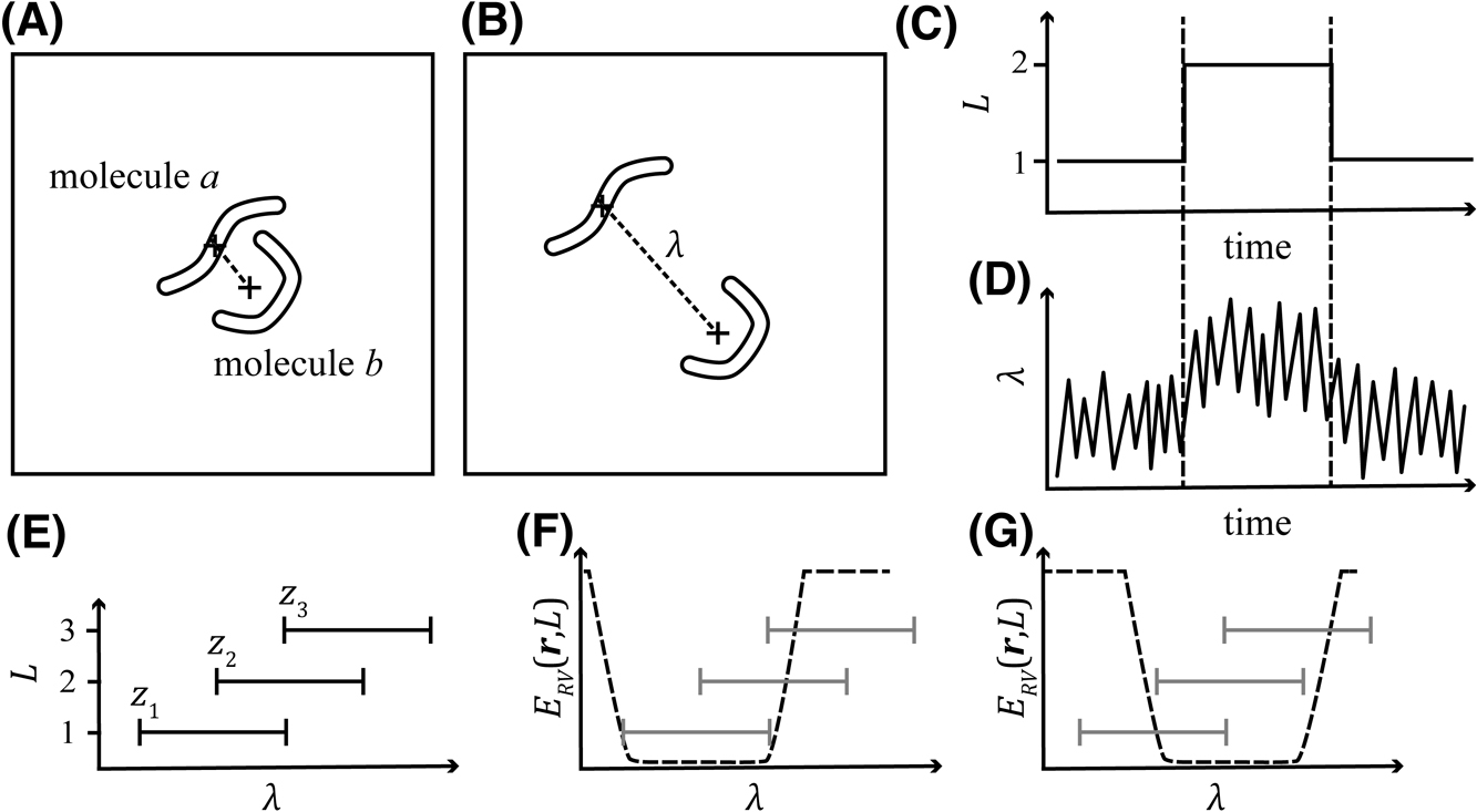
In this class of sampler, the virtual system, which consists of arbitrarily defined discrete states termed as virtual states L, is introduced. The virtual system interacts with the molecular system, or a real system, which is defined as the coordinate and velocity of each particle [r, v]. The phase space of the entire system is defined as [r, v, L]. The state variable L is expressed as an NRc-dimensional integer vector, where NRc indicates the number of reaction coordinates and each axis of the virtual system corresponds to an arbitrarily defined reaction coordinate (λ; Figs. 1A and B). The reaction-coordinate space is divided into several regions overlapping with their neighbors (Fig. 1E), and each region is associated with each virtual state. When the virtual system is in the virtual state L, the real system is confined to a range of reaction coordinates associated (λ∈zL), where zL is defined as the range of λ from [zL]min to [zL]max). After a certain number of sampling steps, the virtual system stochastically transitions to another virtual state L', which is a virtual state neighboring to L (Fig. 1C). Then, the sampling was performed in the range zL' (Fig. 1D). This process is repeated until the end of the simulation.
The virtual system coupled sampler applies the physical system constituted by the following Hamiltonian:
where Eentire(r, L) and K(v) are the potential and kinetic energy terms, respectively. Because the virtual system evolves by the Monte Carlo method, the kinetic term depends only on the real system. Eentire(r, L) is defined by the following equation:
| Eentire(r,L)=ERr+ERVr,L+EVL, | (2) |
where ER(r) and EV(L) are the potential energy terms for the real and virtual systems, respectively. ERV(r, L) is the interaction between the two systems. This term confines the real system into the region zLi, which is associated with the current virtual state Li, for example, the flat-bottom potential (Figs. 1F, G). EV(L) is given as a constant value for each virtual state L, and determines the transition probability between the virtual states. The values of EV(L) for each L can be adjusted to enhance conformational sampling. If the region zL in the reaction-coordinates space is less populated in the canonical distribution, a bias for trapping into this region should be applied by lowering EV(L). The actual procedure for adjusting EV(L) for the case of VcMD is shown in Ref. [30–33].
V-McMD, V-AUS, and VcMD are special cases of the virtual-system coupled sampler. For the V-McMD, the virtual system is defined as one-dimensional (1D) space, the reaction coordinate of which is the potential energy of the real system, and ER(r) is the multicanonical potential defined by the following equation:
| ERr=E(r)+RT ln[PcE(r),T], | (3) |
where E(r) is the potential energy defined by the force field and electrostatic potential in the real system, and Pc(E(r), T) is the canonical distribution of E(r) at temperature T [23]. Conversely, V-AUS applies a structural parameter, for example, the distance between two molecules, to define the 1D reaction-coordinate space, with the adaptive umbrella potential for ER(r).
| ER(r)=E(r)+RT ln [Pcλ,T], | (4) |
where λ is the structural parameter. In this framework, multiple reaction coordinates with a multi-dimensional virtual system can be applied. However because the estimation of the multi-dimensional distribution function Pc(λ, T) would be impractical because of its complexity [24], use-cases of the V-AUS method are practically limited to 1D reaction coordinate space.
VcMD applies an unbiased potential for ER(r).
Instead, conformational sampling is enhanced only by adjusted transition probabilities between different virtual states [30–33].
After the production runs, the canonical ensemble can be obtained by reweighing the resultant ensemble. Because the transitions between different virtual states are biased according to the energy gap of EV(L), the ratio of canonical probabilities of two neighboring virtual states is calculated by the following equation:
| ALj;LiALi;Lj=QcanoLiQcanoLj=exp-EVLj-EVLiRT, | (6) |
where Qcano(Li) is the virtual state-partitioned canonical probability for Lj, and ALj;Li is the transition probability from the state Li to Lj. See Supporting Information of Ref. [33] for more details. In addition, further reweighting is required for the V-McMD and V-AUS methods because sampling in each virtual state is also biased (Eq (3) and (4), respectively). Contrarily, in the VcMD method, sampling in each virtual state is performed under the unbiased manner. Therefore, it is expected that the intersection on the reaction coordinate axis between two neighboring virtual states yields the same distribution. This feature provides the unique protocols for the iterative simulations and sampling as described in Ref. [40].
Coarse-grained simulation
In addition to all-atom simulations, the coarse-grained model can also be applied in myPresto/omegagene. The one-bead-one-residue model with the hydrophobicity scale method [39] is implemented. This method applies a correction reflecting hydrophobicity of the bead to the Lennard-Jones potential:
| Φ(r)=
ΦLJ(r)+(1-λ)ϵ
if r≤216σ
λΦLJ(r)
otherwise
, | (7) |
where Φ(r) is the potential function of a pairwise non-bond interaction with distance r, and ΦLJ is the conventional Lennard-Jones potential with the parameters ε and σ. λ is the scaling factor reflecting hydrophobicity. When λ is unity, Φ(r)=ΦLJ(r). Otherwise (λ is less than unity), the potential is weakened/strengthened for distances which are closer/further than the equilibrium distance, respectively. See the Ref. [39] for details. This potential function has succeeded in reproducing the experimentally determined radii of gyrations of a variety of IDRs and the analysis of liquid-droplet formations [41,42]. For the electrostatic potential calculation, the Debye-Hückel approximation was implemented. Because the previous GPGPU kernel was tailored for all-atom models [22], we modified it to apply the coarse-grained models.
Example
This section describes a VcMD simulation for poly-glutamine (poly-Q) octapeptides, with the coarse-grained model described above as a simple example demonstrating the new functionalities. Because the purpose of this simulation is to provide a simple example that is suitable for a step-by-step tutorial without heavy computations, we do not discuss in detail the molecular phenomena based on the simulation results. More practical applications of the new version of myPresto/omegagene have been reported in our previous studies applying the all-atom VcMD method [29,38]. Applications of the coarse-grained model to investigate higher-order molecular assemblies are partially introduced in Ref. [43], and their details are presented elsewhere.
In this simple example with poly-Q peptides, the reaction coordinate of the 1D virtual system was defined as the distance between the center of masses of these two molecules. The VcMD simulation enhances the sampling of system configurations over a wide range of intermolecular distances. The initial configuration of the molecular system was built by placing two poly-Q octapeptides in a cubic cell with a 60-Å length for each axis. Each poly-Q consisting of eight beads took a fully extended conformation. The system was relaxed in a canonical simulation at 300 K lasting over 105 steps. Ten snapshots were randomly selected from the trajectory and used for the initial structures of the VcMD simulation. In the VcMD simulation, conformational sampling was performed with ten independent runs based on the trivial trajectory parallelization scheme [44] at 300 K. The virtual system was defined as the 1D space based on the distance between the center-of-mass of the two peptides (λ). The range of the λ to be sampled was determined to be 3–30 Å and divided into seven states (Table 1). The parameter set for the hydrophobicity scale model reported by Dignon et al. [41] was applied.
Table 1
Definition of the virtual system
| L |
[zL]min (Å) |
[zL]max (Å) |
| 1 |
3 |
5 |
| 2 |
4 |
6 |
| 3 |
5 |
9 |
| 4 |
6 |
12 |
| 5 |
9 |
17 |
| 6 |
12 |
22 |
| 7 |
17 |
30 |
To determine the potential energy in each virtual state EV(L), conformational sampling using an estimated EV(L) and adjusting EV(L) was iteratively performed until the resultant ensemble converged. Subsequently, a production run was performed with the estimated EV(L). The simulation length of each iteration was 106 steps, and that of the production run was 107 steps. For the first iteration, the potential energies EV(L) for all the virtual states L were set to have a constant value, meaning that the conformational change was not enhanced. This simulation behaved similarly to the unbiased canonical MD. As a result, the resultant ensemble of the first iteration was biased to the configurations with high λ values, and bound configurations were rarely sampled (the red line in Fig. 2A). Then, EV(L) was updated to enhance the conformational changes to the unsampled range of reaction coordinates. After several iterations, the ensemble resulted in a near-uniform distribution over the virtual states, which indicates that a wide range of reaction coordinates was almost equally sampled (Fig. 2B). Based on this estimation of EV(L), a production run was performed. The resultant ensemble can be converted into a canonical ensemble by reweighting each snapshot according to EV(L) (Fig. 2C). In the canonical distribution, under the given potential, dimer conformations were unstable, and the dissociated states showed a more stable potential of mean forces than those in the associated states. The resultant conformational ensemble can be characterized using a variety of analytical methods. Figure 2D presents the free-energy landscape analyzed with the principal component analysis (PCA) for the matrix of 8×8=64 inter-residue distances between the two peptides over 10,000 snapshots. The most stable basin was composed of dissociated configurations (Fig. 2F), which mainly stabilized by the entropic effects. The first principal component axis (PC1) was correlated with the inter-centroid distance between two peptides (the Pearson correlation coefficient was –0.81), and bound conformations were found in the region with high values of PC1 (Fig. 2E).

Conclusions
We presented a new version of the MD simulation engine, myPresto/omegagene. This software is tailored for a series of generalized ensemble approaches termed virtual-system coupled samplers. In this approach, conformational changes in the real system are enhanced by state transitions in the virtual system, which interact with the real system. The new version of myPresto/omegagene provides functionality for the three special cases of the virtual-system coupled sampler, which are V-McMD, V-AUS, and VcMD, and users can choose the appropriate one according to their purpose. In addition, the coarse-grained model with the hydrophobicity scale method and the Debye-Hückel approximation was also implemented. The generalized ensemble approach can be applied to a variety of molecular systems from all-atom explicit-solvent models to coarse-grained models.
This update of myPresto/omegagene includes the documentation for a step-by-step tutorial for VcMD sampling with the coarse-grained model. The input files are attached in “sample/cg_q8” directory of the repository. This example does not demand high computational costs, and users can acquire the necessary skills for the VcMD methods using a laptop computer. For the all-atom model, see “sample/ala3” directory and our previous publication.
Acknowledgments
This work was supported by the Japan Society for the Promotion of Science KAKENHI (Grant Numbers JP16K18526, JP16K05517, and JP20K12069). The computational resources were provided by the HPCI System Research Project (Project IDs: hp190017, hp190018, hp200063, and hp200090), the ROIS National Institute of Genetics, Human Genome Center (the University of Tokyo), and the Research Center for Computational Science, Okazaki, Japan.
Conflicts of Interest
All the authors declare that they have no conflicts of interest.
Author Contributions
KK, JH, TT, and HN designed this study. KK developed the software. KK, JH, and HN developed the methods. HI, SG, and HT performed the calculations. KK and TH wrote the software documentation. All the authors contributed to the writing of the manuscript.
References
- [1] McCammon, J. A., Gelin, B. R. & Karplus, M. Dynamics of folded proteins. Nature 267, 585–590 (1977). DOI: 10.1038/267585a0
- [2] Shaw, D. E., Deneroff, M. M., Dror, R. O., Kuskin, J. S., Larson, R. H., Salmon, J. K., et al. Anton, a special-purpose machine for molecular dynamics simulation. Commun. ACM 51, 91–97 (2008). DOI: 10.1145/1364782.1364802
- [3] Shaw, D. E., Grossman, J. P., Bank, J. A., Batson, B., Butts, J. A., Chao, J. C., et al. Anton 2: raising the bar for performance and programmability in a special-purpose molecular dynamics supercomputer. SC ’14: Proceeding of the International Conference for High Performance Computing, Networking, Storage and Analysis, 41–53 (2014).
- [4] Ohmura, I., Morimoto, G., Ohno, Y., Hasegawa, A. & Taiji, M. MDGRAPE-4: a special-purpose computer system for molecular dynamics simulations. Philos. Trans. A Math. Phys. Eng. Sci. 372, 20130387 (2014). DOI: 10.1098/rsta.2013.0387
- [5] Götz, A. W., Williamson, M. J., Xu, D., Poole, D., Le Grand, S. & Walker, R. C. Routine Microsecond Molecular Dynamics Simulations with AMBER on GPUs. 1. Generalized Born. J. Chem. Theory Comput. 8, 1542–1555 (2012). DOI: 10.1021/ct200909j
- [6] Abraham, M. J., Murtola, T., Schulz, R., Páll, S., Smith, J. C., Hess, B., et al. GROMACS: High performance molecular simulations through multi-level parallelism from laptops to supercomputers. SoftwareX 1-2, 19–25 (2015). DOI: 10.1016/j.softx.2015.06.001
- [7] Waidyasooriya, H. M., Hariyama, M. & Kasahara, K. An FPGA Accelerator for Molecular Dynamics Simulation Using OpenCL. Int. J. Networked Distrib. Comput. 5, 52–61 (2017). DOI: 10.2991/ijndc.2017.5.1.6
- [8] Waidyasooriya, H. M., Hariyama, M. & Kasahara, K. OpenCL-Based Implementation of an FPGA Accelerator for Molecular Dynamics Simulation. Inform. Eng. Express. 3, 11–23 (2017).
- [9] Ishida, H. Molecular dynamics simulation system for structural analysis of biomolecules by high performance computing. Prog. Nuc. Sci. Tech. 2, 470–476 (2011). DOI: 10.15669/pnst.2.470
- [10] Andoh, Y., Yoshii, N., Fujimoto, K., Mizutani, K., Kojima, H., Yamada, A., et al. MODYLAS: A Highly Parallelized General-Purpose Molecular Dynamics Simulation Program for Large-Scale Systems with Long-Range Forces Calculated by Fast Multipole Method (FMM) and Highly Scalable Fine-Grained New Parallel Processing Algorithms. J. Chem. Theory Comput. 9, 3201–3209 (2013). DOI: 10.1021/ct400203a
- [11] Sakuraba, S. & Fukuda, I. Performance evaluation of the zero‐multipole summation method in modern molecular dynamics software. J. Comput. Chem. 39, 1551–1560 (2018). DOI: 10.1002/jcc.25228
- [12] Higo, J., Ikebe, J., Kamiya, N. & Nakamura, H. Enhanced and effective conformational sampling of protein molecular systems for their free energy landscapes. Biophys. Rev. 4, 27–44 (2012). DOI: 10.1007/s12551-011-0063-6
- [13] Iida, S., Nakamura, H. & Higo, J. Enhanced conformational sampling to visualize a free-energy landscape of protein complex formation. Biochem. J. 473, 1651–1662 (2016). DOI: 10.1042/BCJ20160053
- [14] Periole, X. & Mark, A. E. Convergence and sampling efficiency in replica exchange simulations of peptide folding in explicit solvent. J. Chem. Phys. 126, 014903 (2007). DOI: 10.1063/1.2404954
- [15] Abraham, M. J. & Gready, J. E. Ensuring Mixing Efficiency of Replica-Exchange Molecular Dynamics Simulations. J. Chem. Theory Comput. 4, 1119–1128 (2008). DOI: 10.1021/ct800016r
- [16] Sindhikara, D., Meng, Y. & Roitberg, A. E. Exchange frequency in replica exchange molecular dynamics. J. Chem. Phys. 128, 024103 (2008). DOI: 10.1063/1.2816560
- [17] Sindhikara, D. J., Emerson, D. J. & Roitberg, A. E. Exchange Often and Properly in Replica Exchange Molecular Dynamics. J. Chem. Theory Comput. 6, 2804–2808 (2010). DOI: 10.1021/ct100281c
- [18] Rosta, E. & Hummer, G. Error and efficiency of replica exchange molecular dynamics simulations. J. Chem. Phys. 131, 165102 (2009). DOI: 10.1063/1.3249608
- [19] Iwai, R., Kasahara, K. & Takahashi, T. Influence of various parameters in the replica-exchange molecular dynamics method: Number of replicas, replica-exchange frequency, and thermostat coupling time constant. Biophys. Physicobiol. 15, 165–172 (2018). DOI: 10.2142/biophysico.15.0_165
- [20] Shimato, T., Kasahara, K., Higo, J. & Takahashi, T. Effects of number of parallel runs and frequency of bias-strength replacement in generalized ensemble molecular dynamics simulations. PeerJ Phy. Chem. 1, e4 (2019). DOI: 10.7717/peerj-pchem.4
- [21] The PLUMED consortium. Promoting transparency and reproducibility in enhanced molecular simulations. Nat. Methods 16, 670–673 (2019). DOI: 10.1038/s41592-019- 0506-8
- [22] Kasahara, K., Ma, B., Goto, K., Dasgupta, B., Higo, J., Fukuda, I., et al. myPresto/omegagene: a GPU-accelerated molecular dynamics simulator tailored for enhanced conformational sampling methods with a non-Ewald electrostatic scheme. Biophys. Physicobiol. 13, 209–216 (2016). DOI: 10.2142/biophysico.13.0_209
- [23] Higo, J., Umezawa, K. & Nakamura, H. A virtual-system coupled multicanonical molecular dynamics simulation: Principles and applications to free-energy landscape of protein–protein interaction with an all-atom model in explicit solvent. J. Chem. Phys. 138, 184106 (2013). DOI: 10.1063/1.4803468
- [24] Higo, J., Dasgupta, B., Mashimo, T., Kasahara, K., Fukunishi, Y. & Nakamura, H. Virtual-system-coupled adaptive umbrella sampling to compute free-energy landscape for flexible molecular docking. J. Comput. Chem. 36, 1489–1501 (2015). DOI: 10.1002/jcc.23948
- [25] Dasgupta, B., Nakamura, H. & Higo, J. Flexible binding simulation by a novel and improved version of virtual-system coupled adaptive umbrella sampling. Chem. Phys. Lett. 662, 327–332 (2016). DOI: 10.1016/j.cplett.2016.09.059
- [26] Iida, S., Mashimo, T., Kurosawa, T., Hojo, H., Muta, H., Goto, Y., et al. Variation of free‐energy landscape of the p53 C‐terminal domain induced by acetylation: Enhanced conformational sampling. J. Comput. Chem. 37, 2687–2700 (2016). DOI: 10.1002/jcc.24494
- [27] Kasahara, K., Shiina, M., Higo, J., Ogata, K. & Nakamura, H. Phosphorylation of an intrinsically disordered region of Ets1 shifts a multi-modal interaction ensemble to an auto-inhibitory state. Nucleic Acids Res. 46, 2243–2251 (2018). DOI: 10.1093/nar/gkx1297
- [28] Iida, S., Kawabata, T., Kasahara, K., Nakamura, H. & Higo, J. Multimodal Structural Distribution of the p53 C-Terminal Domain upon Binding to S100B via a Generalized Ensemble Method: From Disorder to Extradisorder. J. Chem. Theory Comput. 15, 2597–2607 (2019). DOI: 10.1021/acs.jctc.8b01042
- [29] Higo, J., Kawabata, T., Kusaka, A., Kasahara, K., Kamiya, N., Fukuda, I., et al. Molecular interaction mechanism of 14-3-3ε protein with phosphorylated Myeloid leukemia factor 1 revealed by an enhanced conformational sampling. bioRxiv (2020). DOI: 10.1101/2020.05.24.113209
- [30] Higo, J., Kasahara, K., Dasgupta, B. & Nakamura, H. Enhancement of canonical sampling by virtual-state transitions. J. Chem. Phys. 146, 044104 (2017). DOI: 10.1063/1.4974087
- [31] Higo, J., Kasahara, K. & Nakamura, H. Multi-dimensional virtual system introduced to enhance canonical sampling. J. Chem. Phys. 147, 134102 (2017). DOI: 10.1063/1.4986129
- [32] Hayami, T., Kasahara, K., Nakamura, H. & Higo, J. Molecular dynamics coupled with a virtual system for effective conformational sampling. J. Comput. Chem. 39, 1291–1299 (2018). DOI: 10.1002/jcc.25196
- [33] Hayami, T., Higo, J., Nakamura, H. & Kasahara, K. Multidimensional virtual‐system coupled canonical molecular dynamics to compute free‐energy landscapes of peptide multimer assembly. J. Comput. Chem. 40, 2453–2463 (2019). DOI: 10.1002/jcc.26020
- [34] Jiang, W., Luo, Y., Maragliano, L. & Roux, B. Calculation of Free Energy Landscape in Multi-Dimensions with Hamiltonian-Exchange Umbrella Sampling on Petascale Supercomputer. J. Chem. Theory Comput. 8, 4672–4680 (2012). DOI: 10.1021/ct300468g
- [35] Bartels, C. & Karplus, M. Multidimensional adaptive umbrella sampling: Applications to main chain and side chain peptide conformations. J. Comput. Chem. 18, 1450–1462 (1997). DOI: 10.1002/(SICI)1096-987X(199709)18: 12<1450::AID-JCC3>3.0.CO;2-I
- [36] Higo, J., Nakajima, N., Shirai, H., Kidera, A. & Nakamura, H. Two‐component multicanonical Monte Carlo method for effective conformation sampling. J. Comput. Chem. 18, 2086–2092 (1997). DOI: 10.1002/(SICI)1096-987X(199712) 18:16<2086::AID-JCC12>3.0.CO;2-M
- [37] Sugita, Y., Kitao, A. & Okamoto, Y. Multidimensional replica-exchange method for free-energy calculations. J. Chem. Phys. 113, 6042–6051 (2000). DOI: 10.1063/ 1.1308516
- [38] Higo, J., Kasahara, K., Wada, M., Dasgupta, B., Kamiya, N., Hayami, T., et al. Free-energy landscape of molecular interactions between endothelin 1 and human endothelin type B receptor: fly-casting mechanism. Protein Eng. Des. Sel. 32, 297–308 (2019). DOI: 10.1093/protein/gzz029
- [39] Kapcha, L. H. & Rossky, P. J. A Simple Atomic-Level Hydrophobicity Scale Reveals Protein Interfacial Structure. J. Mol. Biol. 426, 484–498 (2014). DOI: 10.1016/j.jmb.2013.09.039
- [40] Higo, J., Kawabata, T., Kusaka, A., Kasahara, K., Kamiya, N., Fukuda, I., et al. GA-guided mD-VcMD: A genetic-algorithm-based method for multi-dimensional virtual-system coupled molecular dynamics. arXiv. 2006.06950 (2020).
- [41] Dignon, G. L., Zheng, W., Kim, Y. C., Best, R. B. & Mittal, J. Sequence determinants of protein phase behavior from a coarse-grained model. PLoS Comput. Biol. 14, e1005941 (2018). DOI: 10.1371/journal.pcbi.1005941
- [42] Dignon, G. L., Zheng, W., Best, R. B., Kim, Y. C. & Mittal, J. Relation between single-molecule properties and phase behavior of intrinsically disordered proteins. Proc. Natl. Acad. Sci. USA 115, 9929–9934 (2018). DOI: 10.1073/pnas.1804177115
- [43] Kasahara, K., Terazawa, H., Takahashi, T. & Higo, J. Studies on Molecular Dynamics of Intrinsically Disordered Proteins and Their Fuzzy Complexes: A Mini-Review. Comput. Struct. Biotech. J. 17, 712–720 (2019). DOI: 10.1016/j.csbj.2019.06.009
- [44] Ikebe, J., Umezawa, K., Kamiya, N., Sugihara, T., Yonezawa, Y., Takano, Y., et al. Theory for trivial trajectory parallelization of multicanonical molecular dynamics and application to a polypeptide in water. J. Comput. Chem. 32, 1286–1297 (2010). DOI: 10.1002/jcc.21710
