Theory and Results
Preliminary Description of AFM
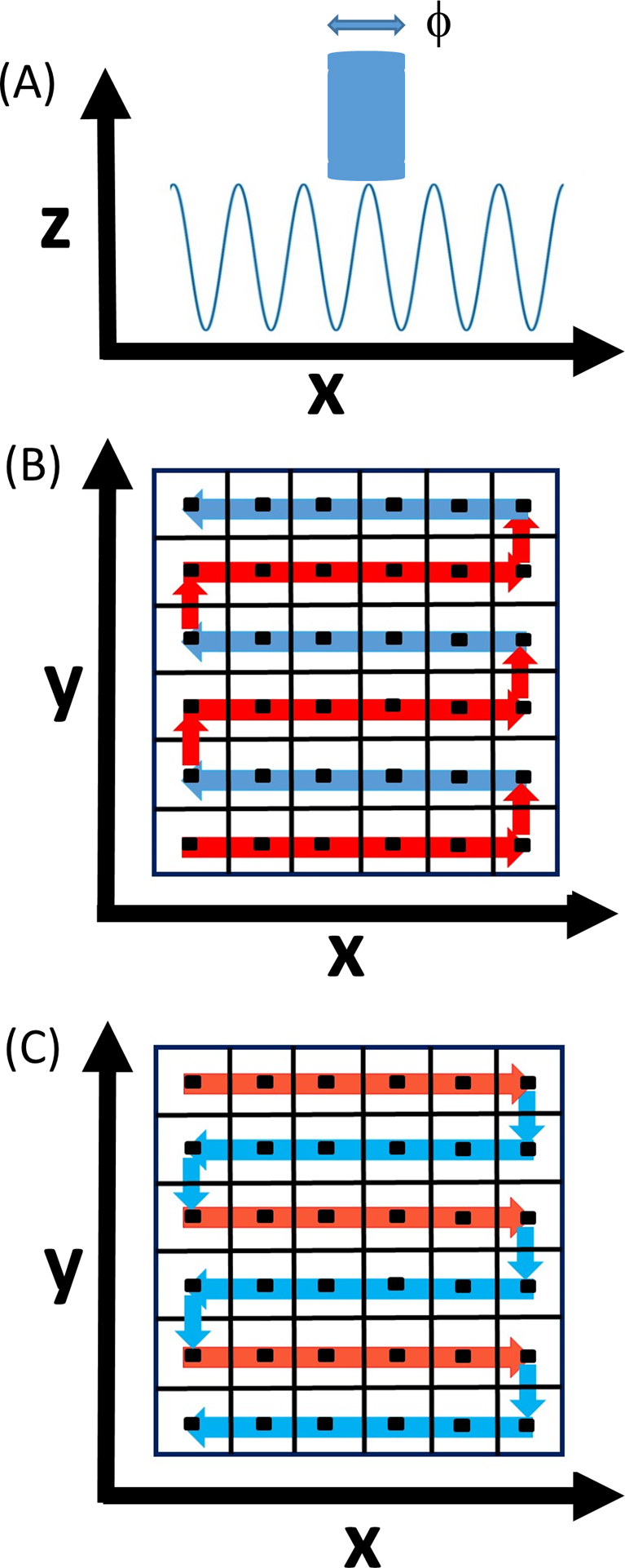
At its core, an AFM is a translatable force gauge equipped with a nanometer-diameter sensing probe [14–16]. The probe, also known as the AFM tip, can be brought into contact with the surface, with the degree of applied force able to be regulated via a feedback control circuit that uses some measurable aspect of the interaction with the sample as input [16,17] (Fig. 2a). The relatively recent development of HS-AFM was made possible through advances in cantilever/tip manufacture and tip/sample spatial control (via use of integrated piezoelectric materials) [12,13]. To enhance sampling rates and the degree of surface coverage, in most modern AFM devices the tip is typically induced to continually oscillate, with the measurement control principles governing the tip/surface interaction based on either amplitude modulation (AM) or frequency modulation (FM) [18]. The vast majority of biologically tailored AFM instrumentation, developed for measuring samples immersed in liquid, operate in the AM mode (also called tapping mode) [16]. Whilst a comprehensive discussion of all of the technical aspects of AFM is beyond the scope of the current work, we present here a number of core points that will prove useful for introducing the present topic of study (Fig. 2b). Important parameters include the maximum side lengths of the x and y axes defining the scanned image area [xmax, ymax], the effective z-axis tip oscillation frequency and tip amplitude pairing, [f, A] and the linear tip scan rates in the x (lateral) and y (vertical) directions, [υX, υY]. When the tip is in contact with the surface, the x linear scan rate, together with the z-axis oscillation frequency determines the effective minimum lateral line sampling distance, xmin=(υX/f). Although not absolutely required, for reasons of simplicity, in this work we set the minimum vertical line sampling distance equal to its lateral counterpart i.e. ymin=xmin.
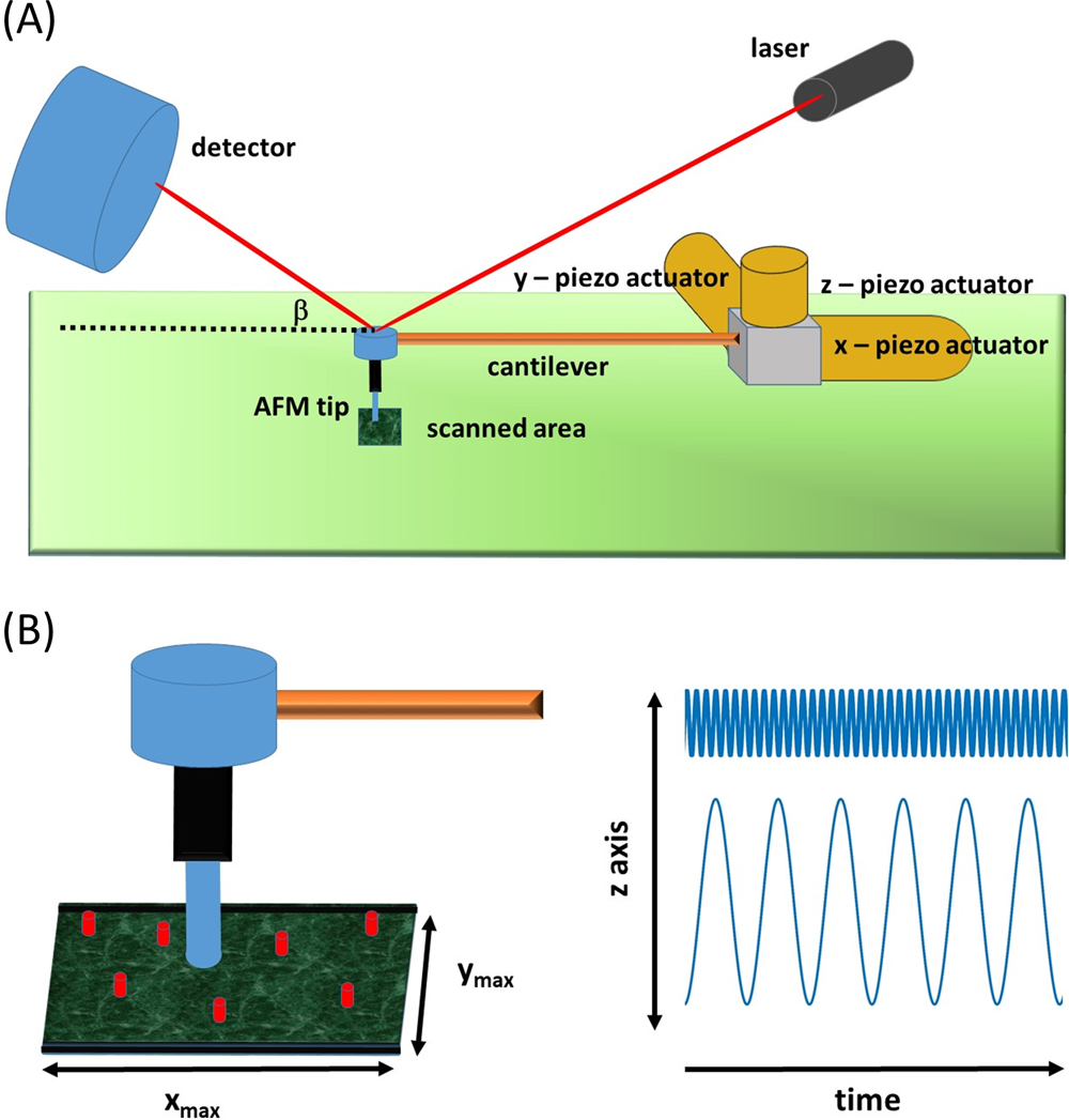
An important step in any AFM experiment is setting the degree of image pixilation [17,19,20] (Fig. 3). A pixel is the basic unit of information within a two-dimensional digital image that is defined by a rectangle of side-lengths xpixel and ypixel and one or more numerical value(s) representing the positional magnitude of the measured variable(s) [21]. Competing factors based on minimizing image size, maximizing signal to noise ratio, maximizing image resolution and minimizing scan time all play a role in dictating the final values of the adopted pixel dimensions [17,22]. The tension between these different determinants can be best understood by comparing the lateral and vertical pixel dimensions (xpixel, ypixel) against the minimum sampling distance (xmin=ymin) and the AFM tip diameter, ϕ (here for simplicity we consider the AFM tip as a right circular cylinder) (Fig. 3a). If we consider the measured variable as the pixel centered surface height, hxy, then we note that when (xpixel, ypixel)>xmin the reported pixel value is the average of the numerous internal values obtained at the sampling interval xmin (Eqn. 1a—with i and j representing running indices for subpoints within the pixel with Nx and Ny describing the number of subpoints in the x and y directions). For static surfaces, such averaging will yield improvements in the signal to noise ratio for locally non-rough surfaces [20,22,23]. Alternatively, when (xpixel, ypixel)=xmin the maximum data driven image pixilation (smallest pixel size possible with maximum number of pixels in image) is achieved such that the reported height is the single measured value at that point (Eqn. 1b).

|
hx,y=∑i=1Nx∑j=1Nyzi,jxpixel/xminypixel/ymin
for (xpixel, ypixel)>xmin
| (1a) |
|
hx,y=zx,y
(xpixel, ypixel)=xmin
| (1b) |
An important distinction in surface sampling can be made when the minimum sampling distance is considered in relation to the tip diameter. For regimes in which xmin≤ϕ we may say that the surface is ‘continuously’ sampled whereas for the situation xmin>ϕ we describe the surface coverage as ‘discontinuously’ sampled. In relation to Eqn. 1 we can set the joint limit of continuous sampling and minimum degree of image pixilation as occurring at the point xmin=ϕ. At this continuous/discontinuous sampling juncture the lateral image resolution, λ, (in the analysis of static samples) will approximately be equal to the minimum sampling distance i.e. λ~ϕ. Neglecting a minor correction for factoring in the feedback control delay, this sampling limit also acts to define the fastest achievable ‘continuous’ lateral scan velocity (Eqn. 2a) which, in turn, defines the fastest continuous vertical scan velocity (Eqn. 2b).
The smallest productive file size that also corresponds to the fastest possible image scanning rate within the continuous sampling regime is given by Eqn. 3.
| Image Sizemin=xmax ymaxϕ2 | (3) |
Having raised some of the factors that jointly optimize the fastest possible scan rates, smallest file size and best resolution we now turn to an examination of how the adopted approach for scanning the surface determines the total scanning time. However, we will revisit the topic of pixilation in the discussion, pointing out some important differences between the averaging process for static and dynamic surfaces.
Raster Scanning Patterns
In HS-AFM the surface is typically interrogated by using raster scanning [24]. Calculation of the return rate of the raster scanning tip to its original position requires knowledge of the scanned image dimensions, the linear scanning rate, the pixilation dimensions and definite assignment of a raster pattern. Although more complex scan patterns are available [24–26] (and discussed in Supplementary 2), we concentrate here on the commonly adopted square grid-based raster pattern applied within the just discussed continuous sampling limit, which we operationally define here as ‘continuous raster’.
Continuous Raster
Continuous scanning applies a fast oscillating, small amplitude vibration to the AFM tip [f,A] under conditions defined by Eqn. 2a such that the maximum scanning velocities and minimum pixilation distance are respectively given by (υx)max=fϕ, (υy)max=fϕ2/xmax and xpixel=ypixel=ϕ (note this also implies that the lateral resolution, λ, for static samples, is approximately λ~ϕ) (Fig. 4a). Raster scanning follows a classical grid pattern with tip motion tracing successive positive and negative directions along the x axis (Fig. 4b, c) [24]. Step increments on the y axis occur in an initially positive direction, until the maximum of the y value range is met, upon which the y axis step increments then become negative for the return raster journey. Due to the back-and-forth nature of the raster scanning process, the tip return rate, Δtret, becomes both a function of pixel position, and direction (positive or negative) of the y step increments. Assuming that the x and y line assignment, lx and ly, and xy-pixel assignment, pX,Y, are set as per a Cartesian graph coordinate system with the maximum line range values for the x and y axes given by lX ∈ (1,xmax/xpixel) and lY ∈ (1,ymax/ypixel), then the time for tip-pixel encounter in the positive, tpos, and negative, tneg, raster scan directions from the respective positive and negative starting positions, are given by Eqn. 4. Other raster patterns are discussed in Supplementary 2.
| tpospX,Y=lX-1xpixelυx+lY-1ypixelυy lY = odd xmaxxpixel-lXxpixelυx+lY-1ypixelυy lY = even | (4a) |
| tnegpX,Y=lX-1xpixelυx+ymaxypixel-lYypixelυy lY = evenxmaxxpixel-lXxpixelυx+ymaxypixel-lYypixelυy lY = odd | (4b) |
For the sake of creating a characteristic AFM temporal constant we define the time taken to complete one tour of the pixel matrix (from the first to the last pixel) as tSCAN. We note that the shortest possible scan time within the continuous sampling limit is given by Eqn. 5a which for the case of a square scanned image area (L=xmax=ymax) is given by Eqn. 5b.
We now use this characteristic tSCAN constant to discuss how AFM sampling rates might be usefully compared with the dynamic processes occurring within the cell membrane.
AFM Assignment for Mobile Cell Membranes
The theoretical potential of an AFM device to measure spatially dependent properties at nanometer levels of lateral resolution and sub-nanometer levels of vertical resolution [16,18] has driven interest into its application to cell biology since soon after the time of its invention [27,28]. Non-penetrative measurements of a cell’s behavior principally involve the high spatial density recording of relatively soft interactions between the AFM tip and the outer cell membrane [28,29]. However, due to its non-equilibrium nature the cell membrane is a dynamic structure that changes over time [30–36]. In terms of how this change occurs, we make a distinction between (i) relatively large-scale (~100nm) gross morphological changes in membrane shape that occur slowly with a time constant, τ1 (~minutes) [e.g. 31,35,37] and (ii) relatively small-scale (~10 nm) changes in the local composition of the two-dimensional membrane fluid, occurring more rapidly with a time constant, τ2 (~milliseconds) [1,38–40]. Although we will define this parameter more carefully in a subsequent section we consider for now that the AFM measurement itself proceeds with a time constant of the order of tSCAN. To a first approximation we compare these different characteristic time constants (τ1, τ2, tSCAN) to define three disparate dynamic regimes of cell membrane motion with each characterized by a corresponding potential capability to relate information between scans via spatial feature assignment.
Regime 1: (τ2<τ1)<<tSCAN → Low confidence
Regime 2: τ2<tSCAN<τ1 → Intermediate confidence
Regime 3: tSCAN≤τ2<τ1) → High confidence
In regime 1, the rate of the AFM measurement is slow in comparison to both the large-scale and small-scale changes in the membrane, resulting in low confidence ability to make spatial assignment between observations. In regime 2 the AFM measurement process is considered fast in relation to the large-scale changes in cell membrane structure but slow in relation to the small-scale changes in membrane composition. This level of resolution is sufficient to assign changes in gross morphological structure, such as for those occurring in cell division [41,42], exosome formation [43], pseudopodia/microvilli projections [44,45] and cell membrane reorganization [29,30,32]. However, the rate of AFM measurement is not sufficient to track and identify molecular level changes in plasma membrane components. Within regime 3 the AFM measurement is considered to operate at a rate comparable to, or faster than, the rate of local redistribution of the membrane contents, thereby potentially allowing for assignment of changes observed between scans. Such a relative temporal difference can be effected in practice by either slowing down the rate of internal redistribution of the membrane (e.g. by chemical fixation [33,46,47]) or by speeding up the rate of the AFM measurement [16,31,48].
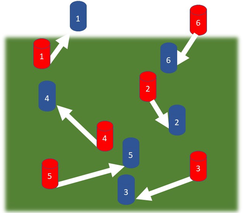
As HS-AFM technologies have continued to improve the tSCAN≤τ2 limit of regime 3 has begun to be approached [16,49,50] such that it is now relevant to investigate the potential for AFM-based assignment of features observed in live cell membranes. To examine this question we have performed both analytical and numerical calculations of an idealized HS-AFM experiment carried out on a region of an otherwise effectively flat cell membrane surface. The measurable difference in some observable property (e.g. vertical height, Δz) is conserved due to a single type of mobile component, denoted as species q, that is capable of random motion defined by a spatially isotropic two-dimensional diffusion coefficient, Dq (Fig. 1). Throughout this paper we will consider a square scanned area on a cell membrane defined by a side length of 10 μm and which contains within it at least one q-type molecule that features an observable topographical projection Δz, and which displays mobility characteristics that comport to either a lipid or peripheral membrane protein [38,51,52], an integral membrane protein [38,53] or a clustered domain of both protein and lipid [54,55]. From experimental measurements of diffusion in artificial vesicle systems, it has been shown that lipids and integral membrane proteins typically show a ten-fold difference in their respective mobilities within the phospholipid bilayer (Dq°~[1,10] μm2s–1) [38,53–57]. This relative difference is somewhat extended in real cell membranes, with the range of absolute mobilities for each decreased by a factor of ten to one-hundred, (Dqreal~[0.01,1] μm2s–1) [38,58]. Theoretical support for this range of experimentally observed values is also given by the Saffman-Delbrück equation (Eqn. 6a) [59,60] which is able to predict the diffusion coefficient of cylindrical rods of radius Rq randomly moving in a continuum two-dimensional fluid of viscosity, η2d, and thickness, H, with the 2d-fluid itself supported in a three-dimensional solvent of viscosity, η3d (with γ denoting the Euler-Mascheroni constant approximately given by 0.5772). Typical values for the two-dimensional membrane viscosity and the three-dimensional solution viscosity at 37°C are η2d=2.7×10⁻¹ kgm–1s–1 and η3d=0.7×10⁻³kgm–1s–1 [61]. The Saffman-Delbrück equation can also be extended to predict the diffusion constant of components in membranes that are densely populated by proteins (defined as a fractional membrane area occupation θ), either over a very short time, DS (Eqn. 6b)—with the fractional area occupation averaged over a local area, <θ>local, or a longer time, DL (Eqn. 6c)—with the fractional area occupation averaged over the total area, <θ> [60–63].
| Dq°=kT4πη2dHlogeη2dHη3dRq-γ | (6a) |
| DqS=Dq°1-2θlocal+2.8238θlocal logeη2dHη3dRq-γ for θlocal≤0.35 | (6b) |
| DqL=DqL1-2.1187θ+1.802θ2-1.6304θ3+0.9466θ4 for θ≤0.7 | (6c) |
An empirical anomalous diffusion relation can be used to fit the transition between DSq and DLq [62] (Table 1).
Table 1
Reduction in diffusion coefficient,
Dq°, of a cylindrical particle existing in the cell membrane as a function of particle radius, and fractional area occupation <θ> or <θ>
local
| Rq/H |
Dq°/Dq°* |
<θ> or <θ>local |
DqS/Dq°** |
DqL/Dq°*** |
| 0.1 |
1 |
0 |
1 |
1 |
| 0.25 |
0.87 |
0.05 |
0.96 |
0.90 |
| 0.5 |
0.77 |
0.1 |
0.92 |
0.80 |
| 0.75 |
0.71 |
0.15 |
0.88 |
0.72 |
| 1 |
0.67 |
0.2 |
0.84 |
0.64 |
| 2 |
0.57 |
0.25 |
0.81 |
0.56 |
| 3 |
0.51 |
0.3 |
0.77 |
0.49 |
| 4 |
0.47 |
0.35 |
0.73 |
0.42 |
| 5 |
0.44 |
0.4 |
|
0.36 |
| 10 |
0.34 |
0.5 |
|
0.25 |
| 50 |
0.10 |
0.6 |
|
0.15 |
| 100 |
0.003 |
0.7 |
|
0.07 |
At 37°C are η2d=2.7×10⁻¹ kgm–1s–1 and η3d=0.7×10⁻³kgm–1s–1. Membrane height H set at 5 nm.
Saffman-Delbrück equation (Eqn. 2a [52]) provides respective estimates Dq° for a lipid (Rq=0.5nm, H=2.5nm) and a mid-sized membrane protein (Rq=2.5nm, H=5nm) in a model lipid bilayer at 37°C as 1.5 μm2s–1 and 0.6 μm2s–1.
* Calculated using the Saffman-Delbrück equation (Eqn. 2a [52]) and normalized with respect to Dq°RqH=0.1.
** Calculated using the equation of Bussell, Koch and Hammer (Eqn. 2b [56]), normalized for Dq°RqH=0.5.
*** Calculated using the equation of Saxton (Eqn.2c [55]).
In the simulations that follow, the scanned image area containing the mobile component is subjected to raster scanning at either a slow, medium or fast scanning speed such that tSCAN ∈ (1,10,100) s. Interpreted through the lens of Eqn. 5 this implies that for a square image scan area of L=10 μm, and a typical AFM device setup with a tip size ϕ ∈ (10, 100) nm, the required AFM cantilever tip oscillation frequencies and tip lateral scan velocities will be in the respective ranges, f ∈ (100, 1×10⁶) and υx ∈ (0.01, 10) mm/s—values which are compatible with current state of the art HS-AFM devices [36,64]. In a corresponding fashion we bracket a range of diffusion constants relevant to the motion of lipids, proteins and protein complexes within a typical phospholipid cell membrane, sampling from Dq ∈ [0.01,0.1,1] μm2s–1.
(i.) What Situations are Assignable?
In order to assign the identity of a mobile particle between successive scans we must first examine an even more basic question that relates to defining which types of mobile systems are indeed ‘assignable’ in the time frame of the measurement. During the course of the first scan, the q-type particle will be initially located at some starting position, r(t0)=[x, y] that corresponds to a pixel coordinate, (pX,Y)start. Depending upon both (i) the initial position of the particle within the scanned region of interest, and (ii) the initial direction of the raster scanning AFM tip upon the first encounter (i.e. positive or negative), the time taken between initial encounter of some particle at pixel position (pX,Y)start and its later possible observation at some pixel coordinate (pX,Y)observe will be defined by the return interval, Δtret, given by Eqn. 7a (for a positive/negative raster scan sequence) and Eqn. 7b (for a negative/positive raster sequence). Some additional useful extensions of the return time come from a pixel-by-pixel consideration of the minimum (Eqn. 7c) or maximum (Eqn. 7d) return time (selected from positive/negative or negative/positive scan directions). All four versions of the return time are shown schematically as a temporal map in Fig. 5.
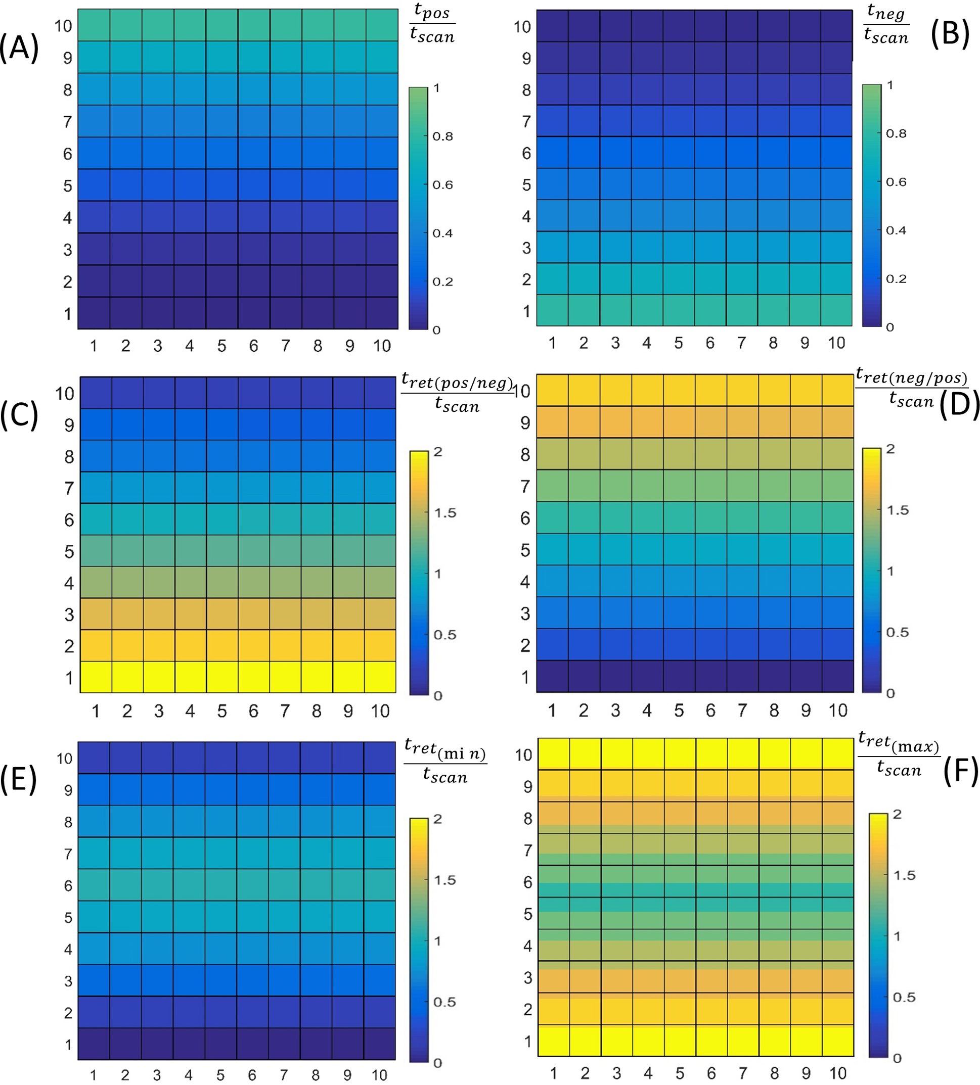
| ∆tretpos/negpX,Yobserve= tscan-tpospX,Ystart+ tnegpX,Yobserve | (7a) |
| ∆tret(neg/pos)pX,Yobserve= tscan-tnegpX,Ystart + tpospX,Yobserve | (7b) |
| ∆tret(min)pX,Yobserve= min(∆tret(pos/neg), ∆tret(neg/pos)) | (7c) |
| ∆tret(max)pX,Yobserve= max(∆tret(pos/neg), ∆tret(neg/pos)) | (7d) |
At a later time, defined by the return period Δtret, the q-type particle’s random (Brownian) motion, can be predicted using the two-dimensional diffusion probability density function, C(r,Δtret), which describes the redistribution of species q to some new position r(Δtret)=[xb, yb] (separated by a distance Δr=|r(Δtret)–r(t0)|) (Eqn. 8a) [61,62]. The probability of finding the particle within a particular square pixel element of area on the plane can be gotten by numerically integrating the probability density function in two dimensions (Eqn. 8b). To assist the numerical solution to approach the continuum limit each pixel was divided into approximately 100 subpixels and the pixel value evaluated via summation of the subpixel probabilities.
| Cr,t=∆tret=14πDite--∆r24Dit | (8a) |
| PpX,Yobserve,t=∆tret≈Cr,t∆xpixel∆ypixel | (8b) |
In the present case the property of assignability relates to the particle’s continuing presence within the image area between successive frames of the AFM scan. Therefore, to answer the question of which situations are assignable we must evaluate the probability, B((pXY)start, t=Δtret) (Eqn. 9) that a particle, initially located at pixel (pXY)start will still be observable within the scan area based on its diffusion coefficient, its initial position and the minimum return time corresponding to its initial position.
| B(pX,Y)start,t=∆tret≈∑X=1X=xmax/xmin∑Y=1Y=ymax/yminPpX,Yobserve,∆tret | (9) |
Figure 6 shows a multi-panel graph showing the evaluation of the assignability, B((pX,Y)start,t) (Eqn. 6) for the three different diffusion coefficients (shown in Table 1) and three different scan times (with return times calculated for each pixel on the basis of Eqns. 7a for the positive, negative scan direction). From Fig. 6 we note that some locations afford a better opportunity for subsequent localization on the return pass than others (when the scanned image area is an open sub-system of a greater area). This position dependence is due to both the position dependent nature of the scan return time and the position dependent propensity of the particle for moving outside the area of observation.

Having established a methodology for assessing assignability (as well as defining realistic limits for what region of the parameter spectrum we could reasonably expect to achieve feature assignment) we now proceed to outline a general method for estimating spatial assignment for any particular mobile system studied by AFM.
(ii.) Spatial ‘Assignment’ for a Single Molecule
Initially we consider the situation of a single mobile q-type molecule comporting to the ‘most assignable’ case described in Fig. 6 i.e. the slowest diffusion coefficient (Dq=0.01 μm2s–1) with the fastest raster scan rate (tSCAN=1 s). The mobile q-type particle is initially located at one of nine positions within a scanned area of side length 10 μm and is probed with a minimal sampling (pixel) distance xmin=100 nm (Fig. 7). Due to the symmetry property associated with the raster scanning and the selected positions we consider only a single directional return time based on the positive-negative transition (Eqn. 7a) trusting the reader to perform any required transformation for other return time possibilities for other raster scanning patterns—see Supp. 2 and 3. As can be seen from Fig. 7a and b when diffusion is relatively slow in relation to the scan rate, the average dispersion of the positional probability is limited, with this dispersion proceeding in a roughly diffusive manner i.e. the mean squared displacement (Eqn. 10a) is approximately linear with time and the average displacement in the x and y directions (Eqn. 10b and c) is very close to zero. Note that Eqns. 10a–c are all ‘renormalized’ to account for the fact that the finite area does not contain the entire probability density after a certain time.

| |∆r|2qeff(t)=∑xminxmax∑yminymaxPpX,Yobserve,t|∆r|2q∑xminxmax∑yminymaxPpX,Yobserve,t | (10a) |
| ∆xqeff(t)=∑xminxmax∑yminymaxPpX,Yobserve,t∆x∑xminxmax∑yminymaxPpX,Yobserve,t | (10b) |
| ∆yqeff(t)=∑xminxmax∑yminymaxPpX,Yobserve,t.∆y∑xminxmax∑yminymaxPpX,Yobserve,t | (10c) |
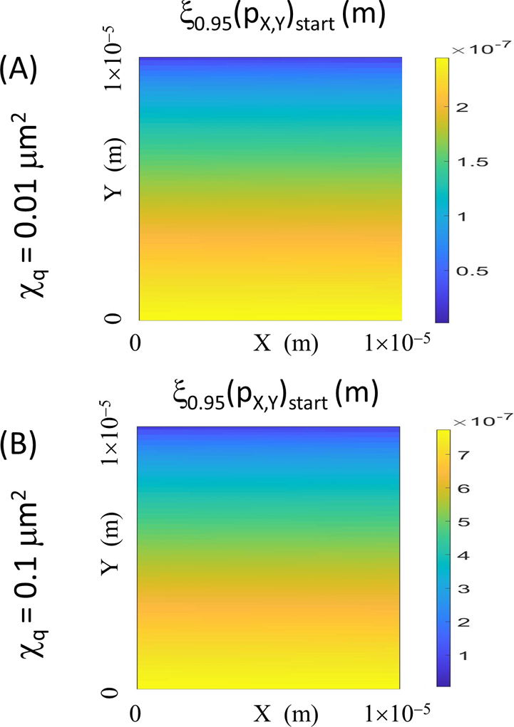
In defining spatial ‘assignment’ we seek to determine the maximum distance, ξ, that a single q-type molecule identified in one movie frame, may travel before we are unsure that it is the same molecule in the next consecutive movie frame, taken after a time interval Δt [5,65–67]. In the ‘diffusion-like’ regime we can answer the question of spatial assignment quite simply by analytically evaluating the integral form of the probability density function (Eqn. 11a) with the added condition that the degree of confidence be set to 0.95 to produce a position dependent estimate of the spatial resolution (Eqn. 11b) (Fig. 7c).
| P(r1(t2)<,t2=∆tret) = ∫θ=0θ=2π∫r=0r=ξCr,t2r.dθ.dr = 1-e-ξ2Dq∆tret(pX,Y) | (11a) |
| ξ0.95≈1.731Dq∆tret(pX,Y) | (11b) |
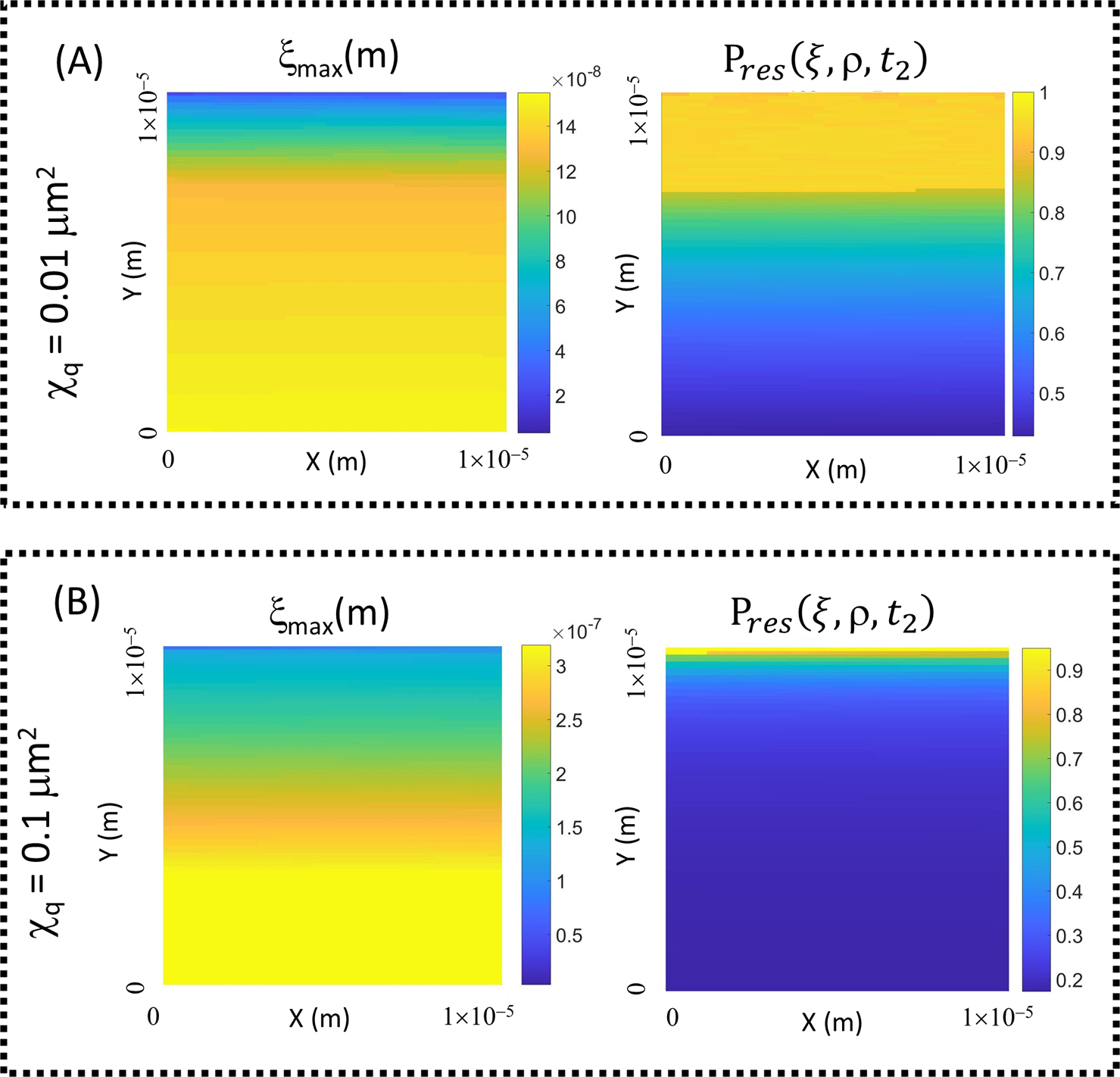
Taking advantage of the scaling property inherent in the diffusion equation we define a composite parameter, χq (where χq=Dq tSCAN), to explore the effect of raster scanning on the measurement as the operative parameters depart from the diffusion-like regime (as shown in Fig. 7) with the results shown in Fig. 8 (noting that the Einstein diffusion relation in two-dimensions <|Δr|2>=4DqΔtret implies that it is the product of the diffusion coefficient and the return time that determines the average squared displacement). We note that when the raster scanning is slow in relation to particle diffusion the reported behavior appears non-diffusive in the sense that the mean squared displacement is not linear in χq and the average x and y displacements significantly deviate from zero (Fig. 8F) (off centered). Aside from these derived parameters one can directly observe that the recorded probability profile becomes distorted and highly asymmetric across the series (Fig. 8A–E). As for the previous section on the question of assignability, the estimation of ‘spatial assignment’ in such circumstances becomes somewhat complex as the recorded profile reflects both a limited set of data (i.e. some particles have left the scanned image area) and a relative velocity effect occurring between the random particle motion and the driven AFM tip. However, plots of the type shown by Fig. 8 are useful for (i) their a priori ability to inform on the soundness of the chosen measurement parameters for feature assignment, and (ii) their a posteriori capability for inferring assignment when a straightforward interpretation is not available (e.g. Fig. 8C–E). To more fully inform on the capability for spatial assignment in AFM based observation of a single particle (Eqn. 8b) we have calculated this value for the range of the composite parameter cases, χq, existing within the diffusive regime (χq=[0.01,0.1] μm2 (Fig. 9).

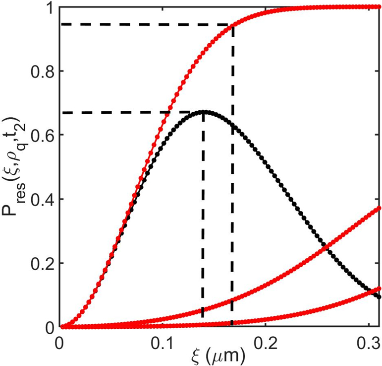
Having considered the question of assignment for a single particle we now determine a practical spatial assignment limit for a q-type particle surrounded by multiple other identical q-type mobile elements, each characterized by the same measurable property (e.g. the height difference, Δz). We consider the q-type elements to be randomly distributed on the surface at an area density, ρq, and are therefore separated from each of their four closest nearest neighbors, on average, by a separation distance dq=1/ρq and their next four closest neighbors by a distance 2dq (see Supp.Fig. 1). In the current work we truncate the probability evaluated in Eqn. 12c to the two nearest shells. In a similar manner to the single particle case, when defining spatial ‘assignment’ for a particle in a high-density arrangement, we seek to determine the maximum distance, ξ, that a single q-type molecule may travel before we are unsure that it is the same molecule in the next frame after a time interval Δt [5,67]. For the present case an equivalent way of stating this problem is to say that we wish to calculate a conditional probability, Pres(ξ,ρq,t2), where t2=Δtret (Eqn. 12a), as the product of the probability that the particle of interest has not moved beyond its resolution window, P(r1(t2)<ξ,t2) (Eqn. 12b). Then the probability that none of the other nearby identical mobile q-type particles (2,3,…,N) have relocated into the area coordinate set, Aξ, encompassing the circle of resolution for particle 1, will be defined by the distance ξ, i.e. ∏J=2j=NP(rj(t2)∉Aξ) (Eqn. 12c).
|
Presξ,ρ,t2=P(r1(t2)<ζ,t2)∏J=2j=NP(rj(t2)∉Aξ) | (12a) |
|
P(r1(t2)<ζ,t2) = 1-e-ξ24Dit2 | (12b) |
|
∏J=2j=NP(rj(t2)∉Aξ) = ∏J=2j=N(1-P(rj(t2)∈Aξ)) | (12c) |
Although the evaluation of the probability shown in Eqn. 12 is simply an exercise in geometry, no analytical solution was readily achievable. In lieu of an exact result a suitable numerical approximation was used (the development of which is shown as Supplementary 1).
Figure 10 shows the spatial assignment parameter, ξ, calculated for a mobile q-type particle characterized by a particular area density, ρq, and diffusion coefficient, Dq. Note that a maximum exists in the probability defining the maximum spatial resolution, ξmax, beyond which point the increasing possibility of substitution/confusion of the central particle for another diminishes confidence in the assignment of its identity. The existence of such a maximum represents a potentially useful way of pre-determining a minimal pixel resolution to the measurement i.e. it represents the most information that can be gotten from the AFM procedure. As this confidence maximum maps to a particular return time it will also be position dependent when conducting raster scanning. To show this we have calculated both the spatial assignment and associated confidence (probability) for each of the composite parameter cases, χq, within the diffusive regime (shown as Fig. 11).
Discussion
Since its invention and application to the measurement of biological samples [14,68] AFM has greatly added to the armamentarium of cell biologists, providing them with a window into molecular level events occurring on, and within, the cell [31,69]. Later developments to increase the speed and resolution of AFM imaging [16,36,64] have made possible the observation of dynamic biological events [e.g. see 29,33,36,40,43,45,70,71]. The current work started with a general question, ‘how confidently can one relate changes observed in consecutive HS-AFM images of a living cell membrane’. To determine an answer, we approached the problem from the simplifying limit of no gross morphological change occurring in the cell structure or position (the regime 2 to regime 3 transition described in this paper). Within this limit, changes in membrane properties, such as local elasticity or topography, result partly (or in whole) from the intrinsic fluidity and heterogeneity of the cell membrane itself [30,38,72,73]. Through a combination of analytical and numerical descriptions of membrane diffusion, raster scanning and image pixilation we have developed systematic methodologies for answering the following three, more specific, questions,
(i) What situations are assignable by AFM?
(ii) How would one confidently assign the identity of a single particle in HS-AFM?
(iii) How does the estimation of spatial assignment change when multiple copies of the particle are present?
With regards to the first question, ‘What situations are assignable by AFM?’, in this work we developed a process (Eqns. 4–9) for estimating the retention of a once encountered molecule within a demarcated region of measurement that exists as an open system within a larger membrane area [30,31,43]. By factoring in the AFM tip scan rate and likely component mobility values, an ‘assignability’ position dependence was determined specifically for the positive-negative return time (Fig. 6), although it is a trivial matter to apply it to any of the other versions of the return time shown in Eqn. 7 as well as for other raster scanning patterns (see Supp. 2 and 3). The simulation process also provided some quantitative backbone to the intuitive understanding that molecules identified towards the edge of the open system have intrinsically lower value in terms of meaningful assignment. Such a systematic approach to the consideration of image ‘assignability’ properties should prove useful to both experimental design and confidence assignment in post-acquisition interpretation of observed structures/properties from different areas of the obtained image [74,75].
To provide an answer to the second question, ‘How would one confidently assign the identity of a single particle in HS-AFM?’, we first developed processes to both, simulate the non-instantaneous AFM-based measurement of a single-particle undergoing random Brownian movement, and identify when the AFM measurement process would report the intrinsically diffusive behavior as not being so (Eqns. 10). When system parameters lie within this characteristic diffusion limit, the integrated form of the diffusion equation may be used to a priori determine a spatial assignment value, ξ, to an arbitrary level of confidence (Eqn. 11). In the present work we used 95% due to its well understood association with normal statistical tables of approximately 2 standard deviations [76]. The practical meaning of ξ0.95 in Eqn. 11 is that it defines the circular area on the membrane, centered around the point of first contact, within which the particle will likely exist at the time of the next AFM measurement. This process could be potentially useful in the design of experiments aimed at analyzing the behavior of distinctive single particles existing within the scanned image (such as for the case of labelled lipids or proteins or relatively rare (in the observation sense) labeled integral membrane proteins, complexes or separate microphases [77]) in two different ways. When high-resolution single particle tracking is the object of study, such information could be used to a priori define the upper limiting value of the image pixilation density and hence the pixel size (i.e. Δxpixel, Δypixel) beyond which potentially important spatial information would be lost. Alternatively, ξ0.95, could be used to inform on minimum pixel spacing when optimizing the high-speed recording of gross cell morphology using a low-resolution, large diameter AFM tip in intermittent raster scanning mode. It is important to realize that the developed formalism [Eqns. 7–10] does not lose its value when the relationship between AFM instrument parameters and the intrinsic membrane dynamics lie beyond the diffusion regime identified by Eqn. 6 and 7. They can still be used to inform on most probable assignment (e.g. Fig. 8C-E) however the problem now loses its circular symmetry and requires that the predicted probability profile be used directly (rather than in the simplified form described in Eqn. 11).
To generate a solution to the third question, ‘How does the estimation of spatial assignment change when multiple copies of the particle are present?’, we modified the single particle assignment calculation (Eqn. 11b) to factor in the conditional probability that a nearby identical particle might wander into the resolution window thereby diminishing our confidence in the assignment (Eqn. 12). This potential for substitution results in a reduced spatial resolution maximum at a lower confidence value (Figs. 10 and 11). In reality, such multiparticle situations are the most likely to be encountered experimentally, due to the fact that the tendency is always for overproduction (either when chemically labeling lipids or proteins or overexpression of genetic constructs) to facilitate easier observation [78,79]. Such density dependent effects on the assessment of required experimental parameters necessary for achieving spatial assignment could be used to inform upon optimal pixilation when the goal is to understand the growth of complexes via self-association of individual protein subunits or alternatively the agglomeration of membrane proteins or lipids into phase separated regions [77,80]. Again, we stress that the general approach (Eqn. 12) is not compromised when experimental diktats mean that the situation is no longer ‘diffusive’ as defined by Eqn. 10 and 12. However, in such cases the problem again loses its symmetry required for simplification and would require evaluation ‘on the fly’ in terms of the asymmetric probability distribution.
Questions Related to Pixilation Choice for Dynamic Membranes
At the beginning of each HS-AFM experiment the user must make a decision upon image pixilation. By formulating the pixilation question in the fashion described in Eqn. 1, this study has teased out some points relating to the differences between static and dynamic surfaces that we now discuss. As noted in the introduction, the joint condition of fastest scan rate and largest pixel size (lowest pixel density) in the continuous sampling limit is set by the oscillation frequency, f, and diameter, ϕ, of the AFM tip, and occurs when xpixel=xmin=ϕ. However, two reasons may prompt an experimenter to set a pixel size that is larger than the minimum lateral and vertical sampling distances (xpixel>xmin; ypixel > ymin) (discussed in the introduction with reference to Figs. 1–3 and Eqn. 1). The first reason involves increasing the signal to noise ratio through oversampling, the second involves decreasing the image file size by combining multiple independent pixels into a larger pixel [21,22,31,49,64]. We note that due to the asymmetric nature of the temporal delay associated with the raster scan process in the vertical and horizontal directions (Eqn.7) any closely positioned sub-pixel pair of measured values in the same lateral scan line, z(x1,y1,t1) and z(x2,y1,t2), will tend to exhibit both a high degree of spatial and temporal correlation for both dynamic and static surfaces. However, similarly closely positioned points in the vertical scan direction, z(x1,y1,t1) and z(x1,y2,tn), will show high spatial and temporal correlation only for static surfaces. Indeed, for dynamic surfaces, any significant redistribution of surface components over the greater time interval associated with completing the vertical component of the raster scanning will diminish the spatial and temporal correlation of the measured variable. Such an understanding implies that rectangular pixilation (with the long axis of the pixel aligned with the lateral direction) may be the preferred choice as a means for achieving both enhanced signal to noise ratios and decreasing image size for dynamic surfaces. Such raster-based spatiotemporal considerations of both pixel construction and pixel-association may also prove important in the execution of the recently posited sub-pixel expansion approach [75] to dynamic surfaces, suggesting at minimum, that different weighting be applied to the interpolations made using x and y-axis components.
Assumptions on Which This Study Rests
Many types of error exist within AFM experiments [16,18]. At the device level errors due to laser intensity fluctuations, quadrant detector Shot noise, cantilever thermal Brownian noise and xyz-piezoelectric creep will all lead to positional error, however these forms of noise are not expected to be significantly time and position dependent and we have neglected their inclusion in the present work. In this study we have placed our focus on positional changes introduced by mobile elements within the membrane [38,51–55]. To develop sufficient traction to move forward we had to make a number of assumptions which, for the sake of clarity we emphasize now. The first, and perhaps most crucial assumption, was that movement within the cell membrane is solely due to its fluid nature and not the result of gross morphological change within the cell. Towards this point, the movement is a general property of all living organisms and cells grown in culture undergo movement at a number of levels [31,81,82]. Cell motion may be due to whole cell walking type processes in which the actin driven lamellipodia project from the anterior membrane to form surface adhesive junctions which can then be used to pull the cell forward [83]. Another type of gross cell movement can be affected by generalized swelling or shrinkage [84]. Examples of more localized forms of movement are those associated with membrane remodeling (endo- or exocytosis) [43,82] or cell division [41]. Nevertheless, a static cell ‘resting state’, in which large scale movements in set sub-regions or by the entire cell, either do not occur or can be rendered negligible through operation of the AFM over a much faster time scale (Regime 2→3), is a known phenomenon for most cell-types, so when observation of cell movement is not the goal of the study, appropriate experimental preparation can minimize the potential complicating effects of movement during the timescale of an AFM measurement [85].
Another major assumption is that the AFM tip does not preferentially interact with mobile particles to influence their trajectory. Such behavior has been noted in the AFM-based measurement of surface defects and ad-atom motion [86,87] as well as in lateral ‘pulling’ experiments of cell membrane receptors by functionalized tips [88,89]. In general, unless interaction between the tip and the mobile surface molecule is a desired aspect of the study any such direct affinity can be eliminated (or at least minimized) by appropriate passivation of the AFM tip and use of appropriate sampling routines—such as the zero-force mode topographical measurement strategies [90]. However, in solution, interactions can also be mediated indirectly as hydrodynamic forces stemming from directed motion of the AFM tip [91]. Such motion can impart kinetic energy to the surrounding solvent, which in turn influences nearby surface molecules [61,92]. The role of such hydrodynamic mediated forces in AFM experimentation has been theoretically studied [91] and may be important if tip motion were to induce non-random behavior in the distributed surface components. If shown to be important, then two of the starting assumptions adopted in this study (diffusive motion of the membrane components and no local deformation of the cell membrane) would need to be modified.
A third major assumption is that the image are is an open system contained within a much larger equivalent membrane environment. Typical eukaryotic cells have diameters in the region of ~20 μm [93] and so this assumption is not unreasonable for many cell-types, however the aspect ratio of some cell types (long and thin fibroblasts or neurons) and the reduced size of others (many prokaryotic cells have diameters 1–5 μm [93]) mean that this boundary condition will not always be the most appropriate selection.
A further assumption relates to the appropriateness of our bounding of parameter space for HS-AFM based interrogation of living cells. Within the development of our argument, we provided experimental and theoretical justification for the selected range of diffusion constants (Table 1). However, we did not fully discuss the reasoning behind our choice of ranges for AFM tip scanning rates, scanned image size and raster patterns. With regard to AFM tip scanning rates, our fastest line scanning rate of 10,000 μm s–1 is representative of values currently achievable using specialist HS-AFM laboratory devices [16,36,43] whilst our slowest line scanning rate of 10 μm s–1 is on par with the vast majority of commercially available AFM devices.
The question of providing spatial bounds for the scanned image is a little more complicated. Potentially, even relatively slow line-scanning rate instruments could be presented as HS-AFM devices if a suitably small image area was chosen (producing sub-second tSCAN frame rates). However, when analyzing cell membrane properties the focus is to measure the cell-scale spatial distribution in the particular property of interest, making sub-micrometer distance scales problematic [28,36]. There are many examples within the AFM live cell membrane literature of AFM image areas with 10 to 40 μm side-lengths observed at frame scan times of several to tens of minutes. We have taken the point of view to use scan times ranging from 1 to 100 seconds to both inform upon results in the published literature as well as forecast what we may expect from next generation devices capable of achieving large area sub-second scan times [36,49].
The final parameter justification relates to our selection of a raster scanning pattern. Different AFM-amenable scanning profiles based on varying sinusoidal patterns, ellipses and decreasing spirals have all been suggested as potentially being superior to the standard back and forth raster pattern described here [24,25] (although we note that these assessments have been solely made in regard to the imaging of static unchanging surfaces). However, the standard raster pattern is a commonly adopted pattern in commercial instrumentation and thus our choice is representative of much published literature [17,49,69]. A related raster scan profile that is used in some laboratory-built AFM devices is the revolving back and forth raster pattern in which, after completion of one positive scan profile, the tip is translated back to the beginning of the image frame [36]. Another type of related scan profile is the uniformly same direction pattern recently introduced by Fukuda and Ando [9] in which both the line and vertical scanning both occur in the same direction throughout the scan. This latter approach has been shown to have the added benefits of simplifying feedback control of the HS-AFM tip and also greatly maintain sample integrity in biological HS-AFM experiments. Both the revolving and uniform direction raster profiles offer potential benefits in producing a regular return time for each pixel independent of its position within the imaged area. However, on the down side, the lack of a reverse scan capability potentially limits the advantages described in Fig. 4 E and F that are associated with the ability to analyze positional information associated with minimum (faster) and maximum (slower) return times. Importantly neither completely mitigate the potential for directional scan bias influencing the symmetry of the assignment envelope (for example see Supplementary 2).
How Our Work Differs from Previous Studies
Although the problem discussed here (AFM measurements of dynamic surfaces) is important for inferring meaning from AFM-based cell biology experiments, there has been surprisingly little work done to address it. Earlier studies by the groups of Greve and Scheuring [6,7] treated a similar problem that related to machine drift between AFM scans but paid less attention to sample component motion within the scan (beyond describing the motion as diffusive). More recently Kubo et al. have applied a Bayesian-based post-processing technique for recreation of more accurate estimates of highly dynamic large biological structures that span multiple pixels within the image [8]. Although the techniques described in that paper refer to specifically to structure estimation, the Bayesian approach described by Kubo et al. [8] could be adapted to the case of feature assignment in both the diffusive (Figs 7A, B) and non-diffusive regimes (Figs 7C-E). However, the major point of this paper is in establishing optimal conditions, prior to experiment, that will maximize data quality and afford easiest interpretability. In terms of the type of problem addressed (i.e. interpretation of dynamic biological surface) this work differs substantially from recent efforts that have concentrated on attaining super high-resolution information from static biological images acquired by HS-AFM methodology e.g. [75]. As the HS-AFM technique improves (becoming faster and less perturbing) the relationship between the relative dynamics of instrument/measurement and biology will change. During this technological evolution it is our belief that the dynamic considerations espoused within the current work will become increasingly important.
Checklist for Experimentalists
At a very practical level this paper has presented simple formalism (easily realizable via spread sheet evaluation) that is both able to provide an estimate of biologically relevant quantities and use the basic parameters of an AFM experiment (e.g. line scanning speed, minimal xy-sampling dimensions, minimum pixilation dimensions and scanned image size) to deduce more useful complex composite instrument terms. These biological and machine related quantities include,
(i) Pixel dependent scan arrival time (Eqn. 4)
(ii) Membrane component motion (Eqn. 6, 7)
(iii) Pixel dependent scan return time (Eqn. 7)
(iv) Positional image confidence (Eqn. 8 and 9)
(iv) Characteristic diffusive regime (Eqn. 10 and 11)
A slightly more difficult implementation of the information included in this paper relates to the specification of density dependent assignment confidence intervals (Eqn. 12, Fig. 11) (but the procedures for its numerical implementation outlined within Supplementary 1 should not be beyond most scientists). To provide some assistance we have developed a standalone application called HS-AFM UGOKU (HS-AFM Users’ Graphical Optimization tool from Kanazawa University) (Supplementary 3). Available upon request from the authors via email and also available for download at the authors’ institutional websites, the HS-AFM UGOKU application takes the scanned image dimensions, the tip diameter and tip oscillation frequency, the dynamic particles dimensions, diffusion constant and surface density and outputs the position and density dependent data described within this paper. Users can employ this tool to pre-optimize their experiment in an iterative graphical fashion. Some screenshots and a basic description of the procedure for usage of the HS-AFM UGOKU software is given as supplementary data to this paper (Supplementary 3).