Image Analysis Tools to Quantify Cell Shape and Protein Dynamics near the Leading Edge

Abstract

We present a set of flexible image analysis tools to analyze dynamics of cell shape and protein concentrations near the leading edge of cells adhered to glass coverslips. Plugins for ImageJ streamline common analyses of microscopic images of cells, including the calculation of leading edge speeds, total and average intensities of fluorescent markers, and retrograde flow rate measurements of fluorescent single-molecule speckles. We also provide automated calculations of auto- and cross-correlation functions between velocity and intensity measurements. The application of the methods is illustrated on images of XTC cells.

Introduction

The advancement of microscopic cell imaging techniques that allow high-resolution visualization of single cells and fluorescently-labeled proteins within cells has driven the development of image analysis methods to quantify cell shape and protein concentrations. In the area of cell motility, a variety of methods have been used to measure the contour and speed of migrating cells using methods such as Level Sets (LSM) (Machacek and Danuser, 2006) Electrostatic Contour Migration (ECCM) (Tyson et al., 2010), Skeletonization (Xiong et al., 2010) and others (Dormann et al., 2002; Bosgraaf et al., 2009; Bosgraaf and Van Haastert, 2010; Huang and Helmke, 2011). This quantification allows correlation of variations in cell shape to local changes in signaling proteins and cytoskeleton protein concentrations within the lamellipodia of eukaryotic cells (Machacek et al., 2009; Ryan et al., 2012). For example, some workers used image analysis methods to characterize oscillations of cell shape (Dubin-Thaler et al., 2004; Machacek and Danuser, 2006; Dubin-Thaler et al., 2008; Machacek et al., 2009; Lam Hui et al., 2012), travelling waves of protrusion propagating along the cell’s arc length (Döbereiner et al., 2006; Machacek and Danuser, 2006; Machacek et al., 2009; Driscoll et al., 2012; Ryan et al., 2012), to measure the retrograde flow velocity of the actin network at the leading edge within lamellipodia (Danuser and Waterman-Storer, 2006; Gardel et al., 2008; Ji et al., 2008; Babich et al., 2012; Ryan et al., 2012; Yi et al., 2012) and to investigate drug-dependent protein mobility and localization within cells (Fujita et al., 2009). Adoption of these methods by the scientific community is becoming widespread but some of these procedures are not available as software, are complex and challenging to implement because they require programming expertise and in some cases may rely on commercial software packages.

In this paper we present a set of flexible image analysis tools to study the protrusion and retraction dynamics of the leading edge of cells adhered to glass slides. We organized these tools into an open source package <http://athena.physics.lehigh.edu/LEAP>. They allow users to measure cellular leading edge speed, local protein concentrations, perform correlation analysis, and measure retrograde flow rates of single-molecule ‘speckles’ over both space and time. A subset of these methods recently allowed us to examine the relationship between cell shape change and local protein concentrations of XTC cells (Ryan et al., 2012). Because this software is designed to run in ImageJ, no commercial software is necessary. The analysis relies on two existing open-source packages, JFilament (Smith et al., 2010) and Speckle TrackerJ (Smith et al., 2011), which are applied to measure cell edge position and single molecule fluorophore positions.

Perhaps the most similar set of image analysis tools is the Quimp (Quantifying Spatio-Temporal Patterns of Fluorescence Intensities at the Cell Membrane) software series (Dormann et al., 2002; Bosgraaf et al., 2009; Bosgraaf and Van Haastert, 2010), which is available as a compiled program. Quimp allows analysis of cell shape and protein concentrations over time similarly to our work. Despite the similarity in approach, there are key differences that make each program better suited in different situations: (i) Our methods allow measurements of cell fragments (such as the image in Fig. 3A that shows only the edge of a cell). This is achieved by use of open active contours to segment part of the leading edge in addition to closed contours for whole cells; (ii) Our use of JFilament and Speckle TrackerJ allows additional manual controls to deal with fitting and tracking errors; (iii) We allow analysis of cell shape combined with retrograde flow measurements and speckle appearance rates; (iv) The methods in this paper are designed to be simple, flexible and to apply to non-motile cells while Quimp includes algorithms to deal with cell movement.

Results and Discussion

Measurement of leading edge position

In our method, cell edges are tracked over time using the JFilament plugin (Smith et al., 2010) to fit closed or open active contours to the intensity gradient at the edge of the cell, see Fig. 1A. Active contours (or snakes) are parametric curves that deform to minimize an energy, which is equal to the sum of an internal energy and an external energy (Li et al., 2009). The internal energy consists of snake stretching and bending terms while the external energy is determined by the image. A measurement of leading edge position of a cell is shown in Fig. 1 using images of an XTC cell expressing LifeAct-mCherry, a fluorescent marker for F-actin, from Ryan et al., 2012. In Fig. 1, for the external energy part of the snake we used the “gradient” option that fits the contour to regions of highest change in intensity, which coincides with the edge of cells (rather than “intensity” that fits contours to regions of highest intensity such as in images of fluorescently-labeled filaments). JFilament also includes “stretching” open active contours; here for open curves we use stretching parameters that approximately maintain the length of the snake.

Fig. 1

Tracking of cell edges allows for measurement of leading edge velocity. (A) Epifluorescence microscopy image of an XTC cell on a poly-L-lysine-coated glass coverslip expressing LifeAct-mCherry, a fluorescent marker for filamentous actin, reproduced with permission from Ryan et al., 2012. Bar, 10 μm. Live cell imaging at 160 nm/pixel and 10 s/frame was carried out as described in (Miyoshi et al., 2006). (B) Contours indicating the cell edge from panel A over 9 different 30 s intervals, using JFilament. (C) Radial velocity is measured as a function of angle from the radial displacement between contours at different consecutive frames. (D) Sample leading-edge velocity measurement at a fixed angle, as a function of time for cell in A. Velocity measurement was taken using M=1 in plugin LE_Velocity. The average standard error of the least squares velocity fit was 9 nm/s.

Tracking of the edge motion in a time lapse movie can be achieved by drawing and fitting an initial active contour along the leading edge. JFilament then propagates the initial contour from a given frame to fit subsequent frames. JFilament allows for manual manipulation of the contours to correct for fitting errors during snake evolution. Fig. 1B shows examples of contours where the cell edge position changes by a few μm over time.

JFilament provides Cartesian coordinates for approximately evenly spaced points along the active contours over time, (x(s, t), y(s, t)), where s is distance along the snake. This represents the position of the edge in the lab frame. For cells (or parts of cells) that remain approximately circular and do not translate over the substrate, as the cell in Fig. 1A (Movie 2 of Ryan et al., 2012), a polar coordinate system is convenient. The plugins included in the package map the contours to polar coordinates about the cell center (x_CM, y_CM). Reparametrization as r(θ, t) is possible when θ is a monotonic function of s. Plugin LE_Radius calculates and saves r(θ, t). All the following plugins assume reparametrization in terms of θ is possible. The distance between snake points along the arc length of the contour is a user-defined variable in JFilament (“point spacing”). We interpolate between recorded points on the active contours so that the leading edge position is measured at 1° intervals.

Measurement of leading edge velocity

Measuring leading edge velocity requires constructing a map between the contours at different time points (Giannone et al., 2004; Machacek and Danuser, 2006; Dubin-Thaler et al., 2008; Machacek et al., 2009; Ryan et al., 2012). This mapping can be complex and depends on assumptions about the physical mechanisms that underlie cell membrane shape evolution. We focused on measuring the radial velocity with respect to a fixed point (x_CM, y_CM), similar to Dubin-Thaler et al. (2004), which is a simple and intuitive measure for circular cells or parts of cells. Plugin LE_Velocity reads an active contour file mapping the leading edge of a cell and calculates the radial velocity at time t_i (where i indicates frame number) as a function of angle θ. Leading edge positions may change very little from frame to frame, depending on sampling rate. Linear regression of the leading edge radial position at a given angle θ over time provides the radial velocity, which is the slope of the linear fit of the leading edge position vs. time (see Fig. 1C). The regression is calculated over the time range [t_i–M, t_i+M], where M>0 is a user-defined value determining how many points are used for the fit. A negative velocity indicates retraction, while a positive velocity indicates protrusion.

LE_Velocity and all plugins discussed here calculate a suggested cell center (x_CM, y_CM) by fitting an arc to the active contours that describe the leading edge position. For every frame we use 100 triplets of points that define an arc and average over all triplets and frames. The cell coordinate center may also be changed manually.

Since we focus on cells whose center does not translocate over time (Dubin-Thaler et al., 2004; Giannone et al., 2004; Döbereiner et al., 2006; Dubin-Thaler et al., 2008; Ji et al., 2008; Machacek et al., 2009; Babich et al., 2012; Yi et al., 2012), applying a fixed cell center and parameterizing the leading edge in terms of θ is a simple and transparent assumption. If a cell is moving over time, or if it is irregularly shaped, a more complicated algorithm would have to be applied on the contour to measure velocities (Dormann et al., 2002; Machacek and Danuser, 2006; Bosgraaf et al., 2009; Bosgraaf and Van Haastert, 2010; Tyson et al., 2010; Xiong et al., 2010). A recent review (Xiong and Iglesias, 2010) discusses the additional assumptions of these methods and possible numerical instabilities in LSM and ECCM.

Measurement of protein intensities near the leading edge

The changing intensity of fluorescently-labeled proteins near the leading edge provides information on the mechanisms of cell signaling, protrusion, retraction, contraction, adhesion, and retrograde flow (Machacek et al., 2009; Ryan et al., 2012). Measuring the image intensity allows us to estimate changes in local protein concentrations over time.

Plugin Intensity_Ribbon uses contours tracking a cell’s leading edge over time to measure intensity in an area near the leading edge as a function of angle, θ, and time. Intensity_Ribbon uses the active contours from JFilament to create two new contours along the cell defined by parameters r_o and r_i (with r_o<r_i) that indicate the offsets of the outer and inner contours from the original contour inward, radially. If r_o=0, then the outer contour will be the original active contour. Negative values of r_o and r_i would be outside the cell. An example with r_o=0 and r_i=5 μm mapped to a cell expressing LifeAct-mCherry from Ryan et al., 2012 is shown in Fig. 2A. Fig. 2A shows the area between the two new contours unbent to a “ribbon” of cell, which is a 2D image I(r, θ, t). Intensity_Ribbon calculates the total intensity as a function of angle and time by integrating:   

$$I_{\mathit{tot}}\left(\theta ,t\right)=\sum _{r=r_a=r_i}^{r_a-t_o}I\left(r,\theta ,t\right)\left(\frac{r}{r_a\left(\theta ,t\right)}\right),$$(1)

where the sum is over pixels with different r, r_a(θ, t) is the position of the cell edge measured by the active contour. The sums of the pixel values are scaled by distance into the cell over its total radius. This weighted summation is applied to account for the distortion of the lamellipodium ‘ribbon’ to a rectangle: as a result of this distortion, the arc-length over an angle range Δθ corresponding to radius r is mapped from a length rΔθ, to r_aΔθ. An example of measured total intensity at a fixed angle over time is shown in Fig. 2A. By varying r_o and r_i it is possible to estimate changing concentrations of proteins over various sections of cell lamellipodia over time.

Fig. 2

Intensity measurements near the leading edge of a cell and correlation of data. (A) Left: Active contours were fit to the leading edge of the cell with JFilament (red). The green line shows a contour 5 μm into the cell (green). Lower panel: magnified Section. Bars are 10 μm (top) and 2 μm (bottom). Middle: The band between the two contours is unfurled into a rectangular ‘ribbon’ of lamellipodium, which is a function of angle θ around the cell, using plugin Intensity_Ribbon. The red and green lines correspond to the inner and outer contours on the left image. Right: Total intensity summed along the width of ribbon as a function of angle (blue). (B) Average LifeAct-mCherry intensity profile of cell in A as a function of distance from the leading edge, calculated using plugin Intensity_Profile and the active contours of panel A. (C) Two-dimensional autocorrelation of leading edge velocity measured from an XTC cell, evaluated with CrossCor_2D and the active contours of panel A. Output matrix of data was graphed in Matlab.

To show how fluorescent intensities vary as a function of distance into the cell from the leading edge, plugin Intensity_Profile uses active contours from JFilament and the output of LE_Velocity to calculate the intensity as a function of distance from the leading edge, angle, and radial leading edge velocity. One output of the plugin is an image stack of the average profile over a specified range of angles, as a function of time. An example is shown in Fig. 2B that shows the average over all the frames of the output profile stack. Another output is a data file of the intensity profile as a function of time and angle. The user may sort or average profiles over these independent variables.

Correlation analysis

The above methods allow measurement of radial leading edge velocity, v_r(θ, t), and total protein intensity I_tot(θ, t) as functions of time and angle (outputs of the LE_Velocity and Intensity_Ribbon plugins). These signals may contain periodic components and correlations that may be obscured by noise and other sources of variability (for example the signal in Fig. 1D has a periodic component). To perform statistical analysis of these measurements, we included plugins to calculate auto- and cross-correlation coefficients.

CrossCorr_2D calculates the cross-correlation coefficients between f(θ, t) and g(θ, t) as function of offsets in angle and time:   

$$c_{f*g}^{2D}\left(\mathrm{\Delta }\theta ,\mathrm{\Delta }t\right)=\sum _k\sum _j\frac{\left[f\left({\theta }_j,t_k\right)-\overline{f}\right]\left[g\left({\theta }_j-\mathrm{\Delta }\theta ,t_k-\mathrm{\Delta }t\right)-\overline{g}\right]}{\left(N-1\right)\left(M-1\right){\sigma }_f{\sigma }_g},$$(2)

where the sum is over time frames (index k) and angles (pixel index j). N and M are the total number of time frames and pixels corresponding to different angles, respectively, for a given Δθ and Δt. f̄ and ḡ are the averages of the respective datasets, and σ_f and σ_g are the corresponding standard deviations. If f and g are the same function then $c_{f*g}^{2D}$ (Δθ, Δt) is an autocorrelation. CrossCorr_1D performs the same calculation as equation (2) but assumes Δθ=0.

An example of an auto-correlation calculation using radial velocities from an XTC cell in Fig. S3 of Ryan et al., 2012 is shown in Fig. 2C. The repeating pattern reflects a periodic process of protrusion and retraction while the diagonal stripes illustrate wave-like propagation of protrusion (Ryan et al., 2012). The cross-correlation coefficients of two different data sets over time yields information about relative time delay between the signals, see Ryan et al., 2012 and Machacek et al., 2009.

Speckle position and retrograde flow measurements

To demonstrate the measurement of single-protein dynamics near the leading edge we use as an example an XTC expressing low amounts of EGFP-Actin, taken from Ryan et al. (2012), see Fig. 3A. The bright spots (“speckles”) show individual EGFP-actin subunits that are polymerized to the filamentous actin network in the cell’s lamellipodium (Watanabe and Mitchison, 2002; Miyoshi et al., 2006; Smith et al., 2011). Because the concentration of fluorescent markers is small, it is possible to distinguish individual molecules. In this figure the leading edge at the time of the snapshot is shown in red. The trajectories in the figure show measurements of the position of individual proteins as a function of time using Speckle TrackerJ (Smith et al., 2011). This plugin has the advantage that it allows users to accurately measure the positions of individual proteins by manually checking individual speckle trajectories, which minimizes tracking errors. The movement of speckles shows the retrograde flow of the actin network away from the leading edge. The position of the speckle was refined by applying the Gaussian Fit model of Speckle TrackerJ.

Fig. 3

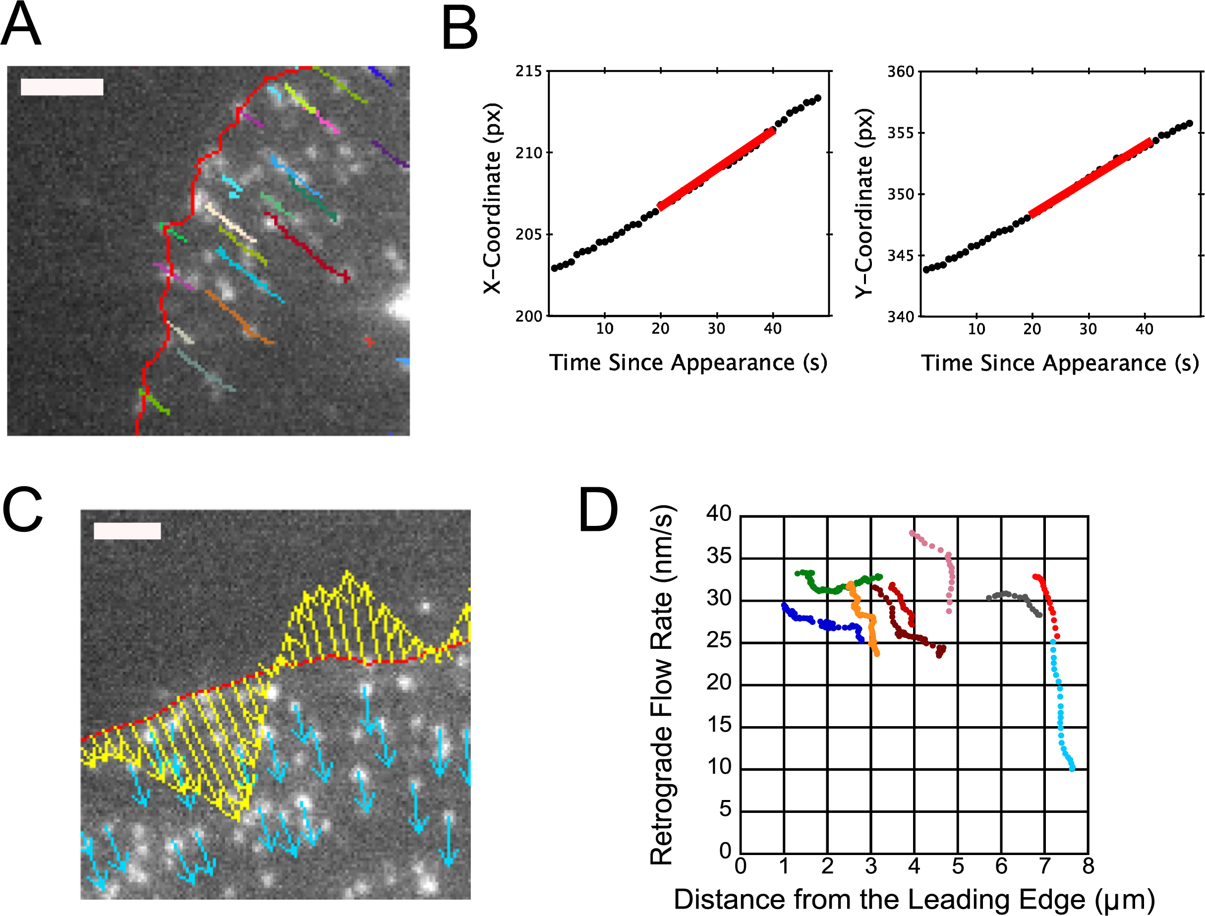
Tracking of single fluorophores via Speckle TrackerJ allows for measurements of retrograde flow rates versus time. (A) Epifluorescence microscopy image of an XTC cell expressing dilute amounts of EGFP-actin. Live cell imaging at 80 nm/pixel and 1 s/frame was carried out as described in (Miyoshi et al., 2006). Single EGFP-actin molecules associated with the filamentous actin network appear as speckles. The position of the leading edge of the cell was measured with JFilament (red line). The tracks of individual speckles tracked with Speckle TrackerJ are shown in multiple colors. We found standard deviations of speckle position fits to be 0.2–0.13 pixels (Ryan et al., 2012). Bar, 1 μm. (B) Example of x- and y-coordinates of one speckle over time. Red line: least squares linear fit over a 20 s time interval for cell from A. This fit is generated automatically in plugin Speckle_Velocity. (C) Example of velocity vectors, generated for XTC cell expressing dilute amounts of EGFP-actin (plugin Speckle_Velocity). Red indicates leading edge position, yellow indicates leading edge velocity, and cyan indicates speckle velocity. Velocity vectors are drawn with 0.5 nm/s per pixel. Bar, 2 μm. (D) Sample speckle velocities as a function of distance from the leading edge for the cell in panel A. Distinct speckles are indicated by color, with each data point corresponding to a different time. Velocity measurement was taken with M=10 in Speckle_Velocity (linear fit over 20 sec as in panel B). Speckle velocities have average error of 2.7 nm/s (Ryan et al., 2012).

Retrograde flow rate can be challenging to measure over time. Some workers developed automated software for images obtained by fluorescent speckle microscopy, where each speckle represents a cluster of molecules (Danuser and Waterman-Storer, 2006). Interpretation of these results however depended on assumptions about the behavior of clusters of molecules: changes in the apparent speckle speed, using a local linear fit, can be due to retrograde flow, polymerization, depolymerization and blinking. Some of the results obtained on retrograde flow by these fully automated tools have been controversial (Danuser, 2009; Vallotton and Small, 2009). Here we consider explicit measurements of the trajectory of single-molecules that leads to better accuracy at the expense of a lower total speckle number. We warn the readers that accuracy of speckle position, image noise, and length of speckle track all need to be carefully considered (Watanabe, 2012).

The ImageJ plugin Speckle_Velocity measures the speed of speckles over time from the output of Speckle TrackerJ and JFilament. Speckle TrackerJ measurements provide the speckle trajectories over time, while JFilament measurements of the leading edge position over time allow the data to be sorted over time, angle, and distance from the leading edge. For the experiment of the cell in Fig. 3A, the movement of an individual speckle is small between time frames. Speckle trajectories are fairly linear over time, both in the x- and y-directions (Fig. 3A, 3B). For a velocity measurement at time t_i (i is the frame number) Speckle_Velocity uses the least squares method to linearly fit the x- and y-coordinates over the time range [t_i–M, t_i+M], where M can be adjusted. An example of these fits is shown in Fig. 3B. The slopes of the fits are the x- and y-components of the speckle velocity, v_x(t) and v_y(t). From these slopes, the net speckle velocity at time t is calculated as   

$$v\left(t\right)=\sqrt{v_x{\left(t\right)}^2+v_y{\left(t\right)}^2}.$$(3)

Speckle_Velocity records the velocity of speckles as function of speckle number, time, speckle lifetime, angle, leading edge speed, and distance from the leading edge. Speckle_Velocity_NoSnakes is an additional plugin that calculates speckle velocities as a function of speckle number and time. It does not require leading edge data. Both plugins generate a velocity vector map, which displays the vector velocities, Fig. 3C.

The fitting interval width M must be chosen large enough so that the displacement of the speckle over the entire interval is larger than the error in position measurement. The accuracy in measuring position can be estimated using the signal to noise ratio (see Fig. 1 in Smith et al. (2011)). The user is advised to examine typical speckle lifetimes and displacements for their system before choosing M, since speckles with lifetimes less than 2M, will not contribute to velocity measurements.

We note another technical issue is the requirement of accurate leading edge position over time. This can be challenging in single molecule fluorescence microscopy images: when fluorophores are dilute the intensity gradient at the cell edge may be too noisy to fit with JFilament. A second fluorescence tag expressed within the cell could be used to guide leading edge movements; alternatively users may apply a moving time-average to enhance the cell edge over time.

Acknowledgments

We thank Matthew B. Smith, Yufei Xia and Sawako Yamashiro for discussions and help with image analysis. This work was supported by the Human Frontiers Science Program Grant No. RGP00612009-C to NW and DV and NEXT program grant No. LS013 from the Cabinet Office, Government of Japan to NW.

References

• Babich, A., Li, S., O’Connor, R.S., Milone, M.C., Freedman, B.D., and Burkhardt, J.K. 2012. F-actin polymerization and retrograde flow drive sustained PLCγ1 signaling during T cell activation. J. Cell Biol., 197: 775–787.
• Bosgraaf, L., van Haastert, P.J.M., and Bretschneider, T. 2009. Analysis of cell movement by simultaneous quantification of local membrane displacement and fluorescent intensities using Quimp2. Cell Motili. Cytoskeleton, 66: 156–165.
• Bosgraaf, L. and Van Haastert, P.J.M. 2010. Quimp3, an automated pseudopod-tracking algorithm. Cell Adhes. and Migr., 4: 46–55.
• Danuser, G. and Waterman-Storer, C.M. 2006. Quantitative Fluorescent Speckle Microscopy of Cytoskeleton Dynamics. Annu. Rev. Biophys. Biomol. Struct., 35: 361–387.
• Danuser, G. 2009. Testing the lamella hypothesis: the next steps on the agenda. J. Cell Sci., 122: 1959–1962.
• Döbereiner, H.-G., Dubin-Thaler, B.J., Hofman, J.M., Xenias, H.S., Sims, T.N., Giannone, G., Dustin, M.L., Wiggins, C.H., and Sheetz, M.P. 2006. Lateral Membrane Waves Constitute a Universal Dynamic Pattern of Motile Cells. Phys. Rev. Lett., 97: 038102.
• Dormann, D., Libotte, T., Weijer, C.J., and Bretschneider, T. 2002. Simultaneous quantification of cell motility and protein-membrane-association using active contours. Cell Motil. Cytoskeleton, 52: 221–230.
• Driscoll, M.K., McCann, C., Kopace, R., Homan, T., Fourkas, J.T., Parent, C., and Losert, W. 2012. Cell Shape Dynamics: From Waves to Migration. PLoS Comp. Biol., 8: e1002392.
• Dubin-Thaler, B.J., Giannone, G., Döbereiner, H.G., and Sheetz, M.P. 2004. Nanometer Analysis of Cell Spreading on Matrix-Coated Surfaces Reveals Two Distinct Cell States and STEPs. Biophys. J., 86: 1794–1806.
• Dubin-Thaler, B.J., Hofman, J.M., Cai, Y., Xenias, Y.H., Spielman, I., Shneidman, A.V., David, L.A., Döbereiner, H.G., Wiggins, C.H., and Sheetz, M.P. 2008. Quantification of cell edge velocities and traction forces reveals distinct motility modules during cell spreading. PLoS One, 3(11): e3735.
• Fujita, A., Shishido, T., Yuan, Y., Inamoto, E., Narumiya, S., and Watanabe, N. 2009. Kinase-Active and Kinase-Defective Abelson Kinase: Requirements of Myristoylation and src Homology 3 Domain. Mol. Pharm., 75: 75–84.
• Gardel, M.L., Sabass, B., Ji, L., Danuser, G., Schwarz, U.S., and Waterman, C.M. 2008. Traction stress in focal adhesions correlates biphasically with actin retrograde flow speed. J. Cell Biol., 183: 999–1005.
• Giannone, G., Dubin-Thaler, B.J., Döbereiner, H.G., Kieffer, N., Bresnick, A.R., and Sheetz, M.P. 2004. Periodic lamellipodial contractions correlate with rearward actin waves. Cell, 116: 431–443.
• Huang, L. and Helmke, B.P. 2011. A Semi-Automatic Method for Image Analysis of Edge Dynamics in Living Cells. Cell. Mol. Bioeng., 4: 205–219.
• Ji, L., Lim, J., and Danuser, G. 2008. Fluctuations of intracellular forces during cell protrusion. Nat. Cell Biol., 10: 1393–1400.
• Lam Hui, K., Wang, C., Grooman, B., Wayt, J., and Upadhyaya, A. 2012. Membrane Dynamics Correlate with Formation of Signaling Clusters during Cell Spreading. Biophys. J., 102: 1524–1533.
• Li, H., Shen, T., Smith, M.B., Fujiwara, I., Vavylonis, D., and Huang, X. 2009. Automated Actin Filament Segmentation, Tracking, and Tip Elongation Measurements based on Open Active Contour Models. Proc. IEEE Int. Symp. Biomed. Imaging., 2009: 1302–1305.
• Machacek, M. and Danuser, G. 2006. Morphodynamic profiling of protrusion phenotypes. Biophys. J., 90: 1439–1452.
• Machacek, M., Hodgson, L., Welch, C., Elliott, H., Pertz, O., Nalbant, P., Abell, A., Johnson, G.L., Hahn, K.M., and Danuser, G. 2009. Coordination of Rho GTPase activities during cell protrusion. Nature, 461: 99–103.
• Miyoshi, T., Tsuji, T., Higashida, C., Hertzog, M., Fujita, A., Narumiya, S., Scita, G., and Watanabe, N. 2006. Actin turnover-dependent fast dissociation of capping protein in the dendritic nucleation actin network: evidence of frequent filament severing. J. Cell Biol., 175: 947–955.
• Ryan, G.L., Petroccia, H.M., Watanabe, N., and Vavylonis, D. 2012. Excitable Actin Dynamics in Lamellipodial Protrusion and Retraction. Biophys. J., 102: 1493–1502.
• Smith, M.B., Li, H., Shen, T., Huang, X., Yusuf, E., and Vavylonis, D. 2010. Segmentation and tracking of cytoskeletal filaments using open active contours. Cytoskeleton, 67: 693–705.
• Smith, M.B., Karatekin, E., Gohlke, A., Mizuno, H., Watanabe, N., and Vavylonis, D. 2011. Interactive, Computer-Assisted Tracking of Speckle Trajectories in Fluorescence Microscopy: Application to Actin Polymerization and Membrane Fusion. Biophys. J., 101: 1794–1804.
• Tyson, R.A., Epstein, D.B.A., Anderson, K.I., and Bretschneider, T. 2010. High Resolution Tracking of Cell Membrane Dynamics in Moving Cells: an Electrifying Approach. Math. Modell. of Nat. Phen., 5: 34–55.
• Vallotton, P. and Small, J.V. 2009. Shifting views on the leading role of the lamellipodium in cell migration: speckle tracking revisited. J. Cell Sci., 122: 1955–1958.
• Watanabe, N. and Mitchison, T.J. 2002. Single-Molecule Speckle Analysis of Actin Filament Turnover in Lamellipodia. Science, 295: 1083–1086.
• Watanabe, N. 2012. Fluorescence single-molecule imaging of actin turnover and regulatory mechanisms. Methods Enzymol., 505: 219–232.
• Xiong, Y. and Iglesias, P.A. 2010. Tools for analyzing cell shape changes during chemotaxis. Integrative Biology, 2: 561–567.
• Xiong, Y., Kabacoff, C., Franca-Koh, J., Devreotes, P.N., Robinson, D.N., and Iglesias, P.A. 2010. Automated characterization of cell shape changes during amoeboid motility by skeletonization. BMC Syst. Biol., 4: 33.
• Yi, J., Wu, X.S., Crites, T., and Hammer, J.A.3rd 2012. Actin retrograde flow and actomyosin II arc contraction drive receptor cluster dynamics at the immunological synapse in Jurkat T cells. Mol. Biol. Cell, 23: 834–852.