Constructing Regression Models with High Prediction Accuracy and Interpretability Based on Decision Tree and Random Forests

Abstract

Models for predicting properties/activities of materials based on machine learning can lead to the discovery of new mechanisms underlying properties/activities of materials. However, methods for constructing models that exhibit both high prediction accuracy and interpretability remain a work in progress because the prediction accuracy and interpretability exhibit a trade-off relationship. In this study, we propose a new model-construction method that combines decision tree (DT) with random forests (RF); which we therefore call DT-RF. In DT-RF, the datasets to be analyzed are divided by a DT model, and RF models are constructed for each subdataset. This enables global interpretation of the data based on the DT model, while the RT models improve the prediction accuracy and enable local interpretations. Case studies were performed using three datasets, namely, those containing data on the boiling point of compounds, their water solubility, and the transition temperature of inorganic superconductors. We examined the proposed method in terms of its validity, prediction accuracy, and interpretability.

1 Introduction

Predicting properties and activities of compounds using machine learning is attracting much research attention. For such predictions, a model is constructed based on properties/activities of existing compounds as determined through experiments and simulations as well as structural descriptors that quantify their chemical structures and the experimental conditions used. Using the model, the properties and activities of new chemical structures can then be predicted without having to perform any experiments. This allows one to select the promising candidates among an almost infinite number of new chemical compositions, thereby improving the efficiency and lowering the costs of research and development efforts. Two examples of physical property/activity prediction models are the quantitative structure–activity relationship (QSAR) model and the quantitative structure–property relationship (QSPR) model. These are regression models between an objective variable y and explanatory variables X. Several methods have been developed for model construction, including the partial least squares (PLS) regression [1], least absolute shrinkage and selection operator (Lasso) [2], and support vector regression (SVR) methods [3]. However, the selection of the model-construction method depends on the dataset to be analyzed.

In 2004, the Organization for Economic Co-operation and Development established the following principles for validating QSAR methods [4]:

1. a defined endpoint

2. an unambiguous algorithm

3. a defined domain of applicability

4. appropriate measures of goodness-of-fit, robustness, and predictivity

5. a mechanistic interpretation, if possible

As described in “3. a defined domain of applicability,” the applicability domain of the model is data domains in which it exhibits good performance. This is because the prediction results will have low reliability in the case of samples whose X values are significantly far from those of the samples used for constructing the model. The applicability domain can be determined using methods such as the k-nearest neighbors classification method [5] or the one-class support vector machine method [6]. In addition, as discussed in “4. appropriate measures of goodness-of-fit, robustness, and predictivity,” in addition to the accuracy of the model with respect to the construction data, its prediction accuracy with respect to external data is also extremely important. Many studies have examined principles 1–4. However, there has been limited research on model interpretability as it pertains to “5. a mechanistic interpretation.” Model interpretation means understanding the relationship between y and X of the model, and improving interpretability can potentially lead to the discovery of new mechanisms and knowledge. However, model prediction accuracy and interpretability exhibit a trade-off relationship, wherein an increase in one means a decrease in the other [7]. For instance, deep neural networks, which are used widely for model construction [8], allow for highly accurate predictions. However, model interpretation in this case is difficult because the model is essentially a black box. If the problem of multi-collinearity does not exist, then the regression coefficients for a linear regression model can be interpreted as the contributions of X to y. On the other hand, the nonlinearity between y and X cannot be expressed owing to the assumption of linearity between them. Thus, the prediction accuracy of a model tends to decrease as one attempts to increase its interpretability. Nevertheless, a model with low prediction accuracy is considered to not have trained the relationship between y and X properly, meaning that its interpretation could also be incorrect. Thus, new methods for constructing models that exhibit both high predictivity and interpretability need to be developed.

Kar et al. constructed a model for predicting the power conversion efficiency of arylamine-based organic dye-sensitized solar cells and interpreted their underlying mechanism based on the variables of the obtained linear regression model and the regression coefficients [9]. Stanev et al. used random forests [10] to construct a prediction model for the transition temperature of superconductors and used it to elucidate the effects of the structure of superconductors on their transition temperature, starting from important variables [11]. In addition, there have been other reports on the interpretation of models with the aim of discovering new mechanisms [12, 13]. Factorized asymptotic Bayesian inference hierarchical mixture of experts (FAB/HMEs) were developed [14, 15] and were applied to extract knowledge on spin-driven thermoelectric materials [16]. Although FAB/HMEs have interpretability, sparsity, and predictive ability of models, nonlinearity between X and y dividing samples into components is limited to squared terms and cross terms of X. The problem of the trade-off between the prediction accuracy of models and their interpretability has not been solved because the interpretation methods are complicated and the prediction accuracy decreases if one focuses on model interpretability.

In this study, to construct QSAR/QSPR models with high prediction accuracy as well as excellent interpretability with the aim of solving the trade-off problem between the two, we combine decision tree (DT) [17] and random forests. A dataset to be analyzed is divided using DT, and then, an RF model is constructed for each subdataset. This approach allows for visual interpretation of the DT while improving the prediction accuracy and results in a more detailed interpretation of the regression model for each subdataset. Since RF is used in modeling each subdataset, any nonlinear relationships can be considered between X and y.

To evaluate the effectiveness of the proposed method, a dataset of boiling point and that of water solubility data are analyzed for various organic compounds. We also investigate the features and drawbacks of the proposed method by comparing its prediction accuracy with those of traditional methods and by examining its interpretability and validity. Then, regression models are constructed for the transition temperature of superconductors, the prediction accuracy of the models is verified, and then, used to discover a new mechanism to explain the characteristics of superconductors based on model interpretation.

2 Methods

2.1 Decision tree (DT)

DT is used to construct a model with a tree-like structure by setting a threshold for each X and repeatedly dividing the dataset based on the magnitude of X. In regression analysis, X and its threshold are determined such that the prediction error is minimized. The sample group at the root of the tree before division and the sample groups after division are called nodes. The nodes that are not divided further in the tree are called the end nodes. In this study, the classification and regression tree algorithm [18] was used as the DT algorithm.

When DT is used for regression analysis, a predicted y value is defined as the average of the sample group for each end node, as shown in Eq. (1):   

${\hat{y}}^{\left(i\right)}=\frac{1}{n}\sum _{i=1}^n{y}^{\left(i\right)}$(1)

Here, n is the number of samples and y⁽ⁱ⁾ and ${\hat{y}}^{\left(i\right)}$ represent the measured y value and the estimated y value, respectively, for the i-th sample. The mean absolute error (MAE) is used to evaluate the function for determining X and its threshold for dividing the dataset:   

$MAE=\frac{1}{n}\sum _{i=1}^n\left|y^{\left(i\right)}-{\hat{y}}^{\left(i\right)}\right|$(2)

With respect to DTs, knowing where to stop the growth of the tree is essential. If too many divisions are made, overlearning is likely to occur, while too few divisions will cause the prediction accuracy to decrease. In this study, the depth of the tree was optimized based on the standard error of the residual of the estimated value after cross-validation (XSE), as shown below.   

$XSE=\sqrt{\frac{\sum _{i=1}^n{\left(e^{\left(i\right)}-\overline{e}\right)}^2}{n\left(n-1\right)}}$(3)

Here, e⁽ⁱ⁾ is the difference between the estimated value of y after cross-validation and the measured value of y for the i-th sample. Further, ē is the average of e⁽ⁱ⁾.

DTs are easy to interpret, given their simple structure. On the other hand, it is known that their prediction accuracy is lower than that of other regression analysis methods because the predictions are based on the average of y. To construct the DTs, we used the tree.DecisionTreeRegressor [19] module in the scikit-learn library.

2.2 Random Forests (RF)

RF is an ensemble learning method based on DTs. The samples and X-variables are selected randomly from the complete dataset to form subdatasets, and a DT is constructed for each subdataset. The prediction accuracies of the DTs differ because each DT is constructed using different samples and X-variables.

In RF, the importance of X can be calculated. The importance of X with respect to the j-th sample can be determined using the following equation:   

$I_j=\frac{1}{k}\sum _T^{}\sum _{t\in T,j}^{}\frac{n_t}{n}\Delta E_t$(4)

Here, k is the number of subdatasets, T is the DT where the X of the j-th sample is used, t is the node in question, n is the number of samples in node t, and ΔE_t is the difference in the value of the evaluation function at node t. The square sum of the residual was used as the evaluation function. The larger the value of I_j is, the more important X is. To construct the RF models, we used the ensemble.RandomForestRegressor [20] module in the scikit-learn library.

2.3 Proposed DT-RF

DT models are readily interpretable but tend to have low prediction accuracy. On the other hand, owing to ensemble learning, RF can improve the prediction accuracy of DT models. However, interpreting the model can be difficult. RF can calculate the importance of X variables with respect to only the entire dataset.

In this study, we propose DT-RF, which combines DT and RF. Figure 1 represents the basic concept of the proposed method. First, a DT is constructed using the dataset to be analyzed. It is expected that this DT model will be easy to interpret but will have low prediction accuracy. Therefore, the samples corresponding to the end nodes of the DT model are used as subdatasets, and a local RF model is constructed for each subdataset. Using this approach, local nonlinear models, which are expected to improve the prediction accuracy, are constructed. In addition, while conventional (global) RF models highlight the importance of X variables corresponding to the entire dataset, this approach allows one to evaluate their effects individually based on their importance with respect to the local RF models. For example, it is possible to evaluate the importance of X variables in sample groups with large/small y values. As discussed above, the proposed method is expected to allow for the construction of property/activity prediction models with both high interpretability and high prediction accuracy.

Figure 1.

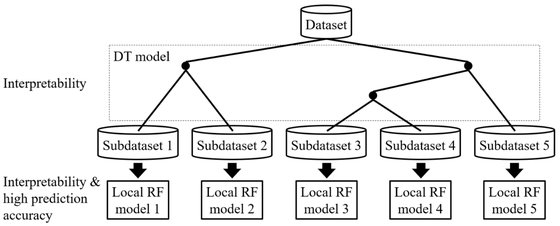
 Basic concept of DT-RF.

3 Results and Discussion

We analyzed three datasets to verify the prediction accuracy and interpretability of the proposed DT-RF. We also compared the performance of the method with those of the PLS, SVR with the Gaussian kernel, RF. The PLS model was constructed using the cross_decomposition.PLSRegression [21] module in scikit-learn while the SVR model was constructed using the svm.SVR [22] module in scikit-learn. The hyperparameters for the SVR model were optimized using the fast optimization method [23]. In this study, the minimum number of samples for each node was set as 40, and the depth of DT was determined to minimize XSE in eq. (3) after cross-validation.

The prediction accuracy was evaluated by double cross-validation (DCV) [24]. Using the training data, the r² and MAE values for the estimated and measured y values were calculated; these are defined as r²_train and MAE_train, respectively. Further, the r² and MAE values for the estimated and measured y values after DCV are defined as r²_DCV and MAE_DCV, respectively.

The first dataset consisted of the boiling points (BP) of 294 organic compounds. In the case of this dataset, y represents the boiling point [°C] of the compound in question while X represents a molecular descriptor that quantifies the chemical structure of that compound. The molecular descriptors were calculated using DRAGON 7.0 [25]. To ensure that the DT could be interpreted easily, only 295 interpretable descriptors, in which complex calculation was not included, were used from all the descriptors. The meaning of the selected descriptors could be understood without complex calculation.

The second dataset was a dataset of the water solubilities (logS) of 1290 organic compounds. Here, y represents the logarithmic value of the water solubility of the compound in question while X represents a molecular descriptor that quantifies the chemical structure of the compound. The molecular descriptors were calculated using RDKit [26]. As was the case for the boiling point dataset, in order to make it easy to interpret the DT, only 127 interpretable descriptors were used.

The third dataset was a dataset of the temperatures [K] of 15542 inorganic compounds at which they exhibit superconductivity (T_C). Superconductivity is a phenomenon wherein the electrical resistance of a compound becomes zero at a certain temperature, and this temperature is called the transition temperature (T_c). Superconductors are an area of active research that has attracted much interest. In 1957, Bardeen et al. [27] proposed the Bardeen–Cooper–Schrieffer (BCS) theory to explain superconductivity at the microscopic level. However, a material with a high transition temperature, which cannot be explained by the BCS theory, was discovered in 1986. Since then, several other high-temperature superconductors have been found [28]. The mechanism responsible for superconductivity at high temperatures is still a matter of debate. For example, in 2017, Sato et al. observed a peculiar phenomenon during a study on metal states [29].

In this study, a DT-RF model was constructed to predict the transition temperature, T_c, of the compounds in the analyzed dataset and also the relationship between the predicted T_c values and the structural information of the compounds. The X-variables were the compositional ratio, average molecular weight (AMW), and the product of the concentrations of each pair of all the constituent elements. As all these X-variables are readily interpretable, all of them were used.

3.1 Analysis of BP dataset

The depth of the DT was set to four, and the minimum number of samples for each node was set to 40. The constructed DT is shown in Figure 2. The DT was plotted using dtreeviz [30]. In each scatter plot, the y- and x-axes represent the boiling point and the X-variable used for dividing the node in the DT, respectively. The values near the arrows are the classification conditions for the X-variable. The BP value at the bottom of each scatter plot of the terminal nodes represents the average boiling point (the estimated value for the DT), and n is the number of samples. The AMW shown in the figure is the molecular descriptor used and was calculated by dividing the molecular weight of the compound by the total number of atoms in it. Based on the plotted DT, we can draw the following conclusions:

Figure 2.

 DT for BP dataset.

(A) When a compound contains only a few non-H atoms and when its AMW is low, its boiling point is low.

(B) When it contains many non-H bonds, its boiling point is high.

(C) When the number of branched structures is small, the boiling point is high.

In other words, (A) states that the boiling point of a compound is low when it has a small structure and contains only a few atoms with high atomic weights. This means that there is a positive correlation between the boiling point of compounds and their molecular weight. (B) is consistent with the fact that the presence of a greater number of hydrogen bonds means a higher boiling point because non-H bonds include those of nitrogen and oxygen atoms. (C) corresponds to the fact that the intermolecular force in a linear structure is greater than that in a branched structure, because of which the former will have a higher boiling point. These conclusions are in keeping with the general theory for explaining the boiling points of compounds. Thus, the interpretation of the DT constructed in this study is appropriate.

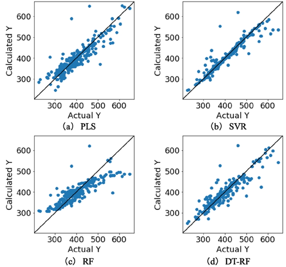
Table 1 shows a comparison of the prediction accuracy of the DT-RF model and those of other conventional methods. With respect to DCV, outside cross-validation refers to leave-one-out cross-validation while inside cross-validation refers to five-fold cross-validation. As shown in Table 1, the DT-RF model exhibited higher r²_train and r²_DCV values and smaller MAE_train and MAE_DCV values than those of the PLS and RF models. Thus, it was superior in terms of both the goodness-of-fit and the prediction accuracy. Further, its r²_train and r²_DCV values were slightly higher and its MAE_train and MAE_DCV were lower than those of the SVR model. Figure 3 shows the scatter plots for each method; the y-axis represents the value of y estimated using DCV and the x-axis represents the measured value of y. A greater number of samples lie near the diagonal in the case of DF-RF than for PLS and RF, meaning that the predictions made by the former were more accurate in general. Further, while more samples lie near the diagonal in the case of the SVR model, this model also exhibited larger prediction errors for the samples with high boiling points. This was presumably because the SVR model was constructed using all the samples in the dataset, which contained few samples with high boiling points. In contrast, the samples with similar boiling points were grouped together in the case of the DT-RF model, and submodels were constructed for each node, which supposedly allowed adopting to samples with local values.

Table 1.  Prediction results for BP dataset

Method	r2train	MAEtrain	r2DCV	MAEDCV
PLS	0.890	16.0	0.823	20.5
SVR	0.961	3.67	0.836	13.8
RF	0.946	12.1	0.700	27.7
DT-RF	0.971	7.60	0.847	17.2

Figure 3.

 Results of DCV for BP dataset.

Figure 4 shows the plot in Figure 3(d) for each node. Node10 contains many samples with high boiling points, and thereby large values with few samples in the entire dataset could be predicted with high accuracy. A similar observation can be made in the case of the samples with low boiling points based on node2 and node4. However, for each node, the prediction results for the samples with boiling points significantly different from those of the other samples were poor. This is because of the large number of samples in the dataset. These samples were not classified correctly by the DT. Hence, there is a chance that the prediction accuracy would be worse than that of the models constructed using all the samples.

Figure 4.

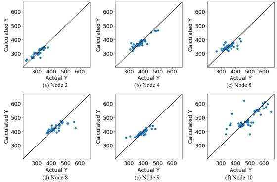
 Results of DCV for each node for BP dataset.

Next, we attempted to interpret the DT-RF model based on the importance of the submodel variables. Figure 5 shows the importance of the seven most important variables for each node in the DT-RF model while Figure 6 shows the top seven most important variables in the RF model (for comparison). In both bar charts, the y-axis represents the selected X-variables and the x-axis represents the variable importance. In node 2 of the RF model, all the important variables, such as MW, are the descriptors related to the molecular size of the compounds. Similarly, many descriptors related to the molecular size were also selected in nodes 4 and 5. However, nHDon (number of N and O donor atoms for H-bonds) was selected as an important variable in node 4 while O-057 (number of O atoms in OH group in phenol, enol, or carboxyl groups) and nRCOOH (number of carboxyl acid groups) were selected in node 5. These three descriptors are variables related to hydrogen bonds. In addition, nROH (number of hydroxyl groups) is an important variable in nodes 8 and 9. In node 8, nROH is more important than nHDon, suggesting that nROH was suited better for predicting the boiling points of the samples in node 8. In the case of node 10, the higher the number of non-H atoms, the higher the boiling point was, as shown in the scatter plot in Figure 3(d). This confirmed the importance of nBO, which is shown in Figure 5. There are several descriptors as important variables in this figure that are not present in Figure 6. This suggested that the locally important variables that could not be determined with a model constructed using all the samples could be extracted successfully by first grouping the samples with similar chemical structural properties and then constructing RF models for each of these groups.

Figure 5.

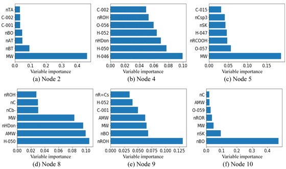
 Importance of variables of BP dataset for focal RF models.

Figure 6.

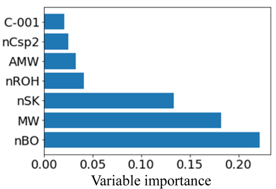
 Importance of variables of BP dataset for global RF model.

3.2 Analysis of logS dataset

While constructing the DT, the tree depth was set to four, and the minimum number of samples for each node was set to 40. The constructed DT is shown in Figure 7. In each scatter plot, the y- and x-axes represent the logS value and the X-variable used for dividing the DT, respectively. The logS value at the bottom of each scatter plot of the terminal nodes represents the average logS value (the estimated value of the DT), and n is the number of samples. MollogP is the Wildman–Crippen LogP and MolMR is the Wildman–Crippen MR. With respect to the DT, the smaller MollogP is, the larger logS is. Further, the smaller MolMR is, the larger logS is. This interpretation is consistent with the general theory for explaining the water solubility of compounds, which states that the lower the hydrophobicity of a compound is, the higher its hydrophilicity will be. Further, organic compounds with a large molecular weight will exhibit low water solubility. Therefore, the validity of the model was confirmed for the boiling point data as well.

Figure 7.

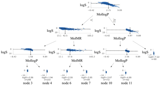
 DT for logS dataset.

Table 2 compares the prediction accuracy of the DT-RF method with those of the other methods. With respect to DCV, outside cross-validation is leave-one-out cross-validation while inside cross-validation is five-fold cross-validation. As shown in Table 2, compared with PLS and RF, DT-RF showed higher r²_train and r²_DCV values and lower MAE_train and MAE_DCV values. This means that it was superior in terms of both goodness-of-fit and prediction accuracy. Further, its r²_train and r²_DCV were similar to those of SVR while its MAE_train and MAE_DCV values were larger.

Table 2.  Prediction results for logS dataset

Method	r2train	MAEtrain	r2DCV	MAEDCV
PLS	0.883	0.540	0.461	0.785
SVR	0.984	0.175	0.879	0.505
RF	0.918	0.441	0.825	0.687
DT-RF	0.971	0.257	0.875	0.550

Figure 8 shows scatter plots for each method; the y-axis represents the value of y estimated by DCV and the x-axis represents the measured value of y. In the case of SVR, RF, and DT-RF, a large number of samples are distributed near the diagonal, indicating that the overall prediction accuracy of these methods was good. Figure 9 shows the plot in Figure 8(d) for each node. In nodes 6 and 7, the samples are distributed horizontally, and the prediction accuracy is lower than that for the other nodes. This is possibly because the RF model did not fit the model-construction data well, owing to the wide range of the y values and the small number of samples with large/small y values. In the cases of nodes 3, 4, 10, 11, and 12, a large number of the samples lie near the diagonal, indicating that at least the magnitude of the y value is expressed.

Figure 8.

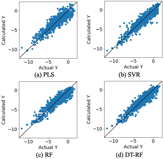
 Results of DCV for logS dataset.

Figure 9.

 Results of DCV for each node for logS dataset.

Next, we attempted to interpret the DT-RF model based on the importance of the submodel variables. Figure 10 shows the importance of the seven most important variables for each node in the DT-RF model, while Figure 11 shows the importance of the seven most important variables in the RF model for comparison. In both bar charts, the y-axis shows the selected X-variable and the x-axis shows the importance of the variable. As can be seen from Figure 10, MollogP and MolMR were important in all the nodes. Further, Figure 11 shows that these two had the greatest effect on the prediction accuracy. In addition, descriptors related to N and O, such as NOCount (the number of N and O atoms) and fr_Al_OH_noTert (the number of nontertiary OH groups), were important in both models. This suggests that both models were able to “learn” the fact that compounds with structures that can form hydrogen bonds are likely to exhibit high water solubility. In addition, many descriptors related to the molecular weight were also important. Moreover, in the case of a few nodes, the variables related to aromatic rings were considered important, such as fr_aniline in node6, NumArimaticCalbocycles (the number of benzene aromatic rings) in node 11, and NumAromaticRings (the number of aromatic rings, including heteroaromatic rings) in node 12. Thus, based on an analysis of the logS data using the DT-RF model, we could determine the locally important variables, in contrast to the case for the RF model, which was constructed using all the samples.

Figure 10.

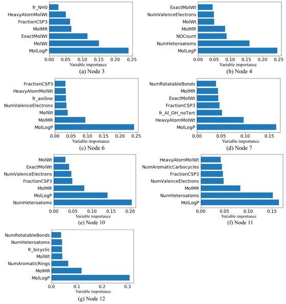
 Importance of variables of logS dataset for local RF models.

Figure 11.

 Importance of variables of logS dataset for global RF model.

3.3 Analysis of inorganic superconductor dataset

While constructing the DT, the tree depth was set to seven, and the minimum number of samples for each node was set to 200. The constructed DT is shown in Figure 12. In each scatter plot, the y- and x-axes represent the transition temperature (T_c) and the X-variable used for dividing the DT, respectively. The values near the arrows are the classification conditions for the X-variable. The T_c value at the bottom of each scatter plot of the terminal nodes represents the average T_c value for the node (the estimated value for the DT), and n is the number of samples. This DT was interpreted as described below:

Figure 12.

 DT for T_c dataset.

A) When the product of the composition ratio of Cu and that of O is smaller than 0.005, T_c is likely to be low.

B) When the product of the composition ratio of Ba and that of Ca is 0.011 or greater, T_c is likely to be high.

C) When the product of the composition ratio of Ba and that of O is 0.0486 or greater, T_c is likely to be high.

The first high-temperature superconductors with a T_c higher than 77 K are copper oxides. The first classification condition, (A), also suggests that the composition of the compound must be that corresponding to copper oxides for it to have a high T_c. Furthermore, high-temperature superconductors have also been found in the La-Ba-Cu-O, Ba-Y-Cu-O, Bi-Sr-Ca-Cu-O, Tl-Ba-Ca-Cu-O, and Hg-Ba-Cu-O systems; these would be in keeping with conditions (B) and (C). Therefore, it can be concluded that the DT correctly represents the relationship between the composition of a compound and the likelihood that it will be a high-temperature superconductor.

Table 3 compares the prediction accuracies of the PLS, RF, and DT-RF models. With respect to DCV, both outside cross-validation and inside cross-validation are five-fold cross-validation. The SVR model could not be used, as the number of samples was too high, and the memory installed on the PC used proved to be inadequate for the calculations. However, as can be seen from the table, compared with the PLS model, the DT-FR model was superior in terms of all the evaluation indices. The MAE_train value of the RF model was smaller, suggesting that it is more suitable to date for model construction. However, the r²_DCV and MAE_DCV values of the two models were not different, indicating that there should be no significant differences in their prediction accuracies in the case of external data. On the other hand, there was a significant difference in the prediction accuracy, as evaluated using r²_DCV and MAE_DCV, of the linear PLS model and those of the nonlinear RF and DT-RF models. This suggests that there exist nonlinear correlations between the explanatory variables and the response variable, T_c.

Table 3.  Prediction results for T_c dataset

Method	r2train	MAEtrain	r2DCV	MAEDCV
PLS	0.752	11.9	-30.7	17.7
RF	0.990	1.85	0.869	7.24
DT-RF	0.923	5.14	0.842	7.96

Figure 13 shows the scatter plots for PLS, RF, and DT-RF; the y-axis represents the value of y estimated by DCV and the x-axis represents the measured value of y. As can be seen from Figure 13(a), a large number of samples lie away from the diagonal, indicating poor prediction accuracy. On comparing Figures 13(b) and (c), it can be seen that, in the case of the DT-RF model, there are several samples with large errors whose measured value is approximately 50–125 K and estimated value is approximately 0 K. One reason for this discrepancy could be that these samples were grouped into a node with a low average T_c. Thus, the prediction results were affected by the low values during the submodel construction process. On the other hand, there are several samples that have measured values of approximately 130–140 K but whose estimated values in the case of the RF model were off by a large margin but close in the case of the DT-RF model. This suggests that the prediction accuracy of DT-RF was higher for the samples with high-T_c values.

Figure 13.

 Results of DCV for T_c dataset.

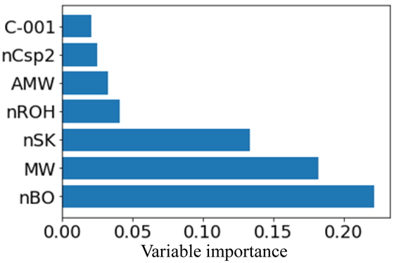
Next, we attempted to interpret the DT-RF model based on the importance of the submodel variables. Figure 14 shows the importance of the seven most important variables for each node in the DT-RF model. For node 21, which had an average T_c of 68.44 K, variables such as Y×Sr, La, Cu×Ca, and AMW were selected. Y-based copper oxide superconductors have been investigated extensively since they were first discovered and are known to exhibit T_c values higher than 90 K. Y×Sr is the third-most important variable. Thus, in the case of Y-based copper oxide superconductors, the presence of Sr has a determining effect on T_c. For node 21, AMW is the most important variable. As can be seen from Figure 14, whether La (which has a high atomic weight at 138.9) and Ba (which also has a high atomic weight at 137.3) are present or not also has a determining effect on T_c. For node 25, which has the highest average T_c at 107.39 K, X-variables related to the presence of Hg were important; these variables were not found in the other nodes.

Figure 14.

 Importance of variables of T_c dataset for local RF models

Hg-based superconductors are among the inorganic superconductors being explored. In 1993, a Hg-Ba-Ca-Cu-O-based high-temperature superconductor with a T_c of 133.5 K was discovered [31]. Its constituents are among the elements corresponding to the important variable for node 25. In addition, the fact that Hg×Tl is a highly important variable suggests that whether Tl is present or not also has a determining effect on the T_c value of Hg-based superconductors. In node 32, for which the average T_c is 76.34 K, the important variables correspond to the presence of La and Ca, which have a determining effect on the T_c values for the compounds in this node. In the case of the nodes with a large number of high-temperature superconductors, such as nodes 25 and 32, the presence of both Ba and Ca was important. Many of the high-temperature superconductors found to date contain both elements. These results suggest that the presence of both Ba and Ca results in a high T_c. On the other hand, while many high-temperature superconductors contain elements such as Y and Bi, these were not discovered by the DT-FR model. This could be owing to poor sample classification by the DT. In the absence of proper classification, the X-variables corresponding to Y and Bi remained unselected. More accurate classification may have resulted in the case of a different set of important variables. However, at the same time, it may also have reduced the prediction accuracy as fewer samples would be available for submodel construction.

Next, we simulated inorganic compounds using the elements from the model-construction data, determined the values of the corresponding X-variables, and predicted their T_c values using the constructed DT-RF model. During the simulation, the number of different elements and number of atoms in the compounds were set to 4–6 and 6–10, respectively, so that they lay within the range of the model-construction data. The type and number of elements and the number of atoms were randomly selected from within this range. The inorganic compounds were simulated as per these guidelines. Figure 15 shows histograms of the T_c values predicted using the DT-RF model. The upper histogram shows the prediction results for all 10152 compounds while the lower histogram is a magnified view of the high-T_c region. The inorganic compounds that showed potential as high-temperature superconductors corresponded to the following terminal nodes, which are arranged based on their average value: nodes 25, 32, and 21. Because the RF model predicted T_c values through ensemble learning based on DT models, all the predicted T_c values lay within the range of the T_c values in the training samples, which was the limitation of the proposed DT-RF. For this reason, no candidate exhibited a T_c higher than that of the training samples. However, the simulated compounds can be expected to exhibit high-temperature superconductivity, given the prediction accuracy of the DT-RF model.

Figure 15.

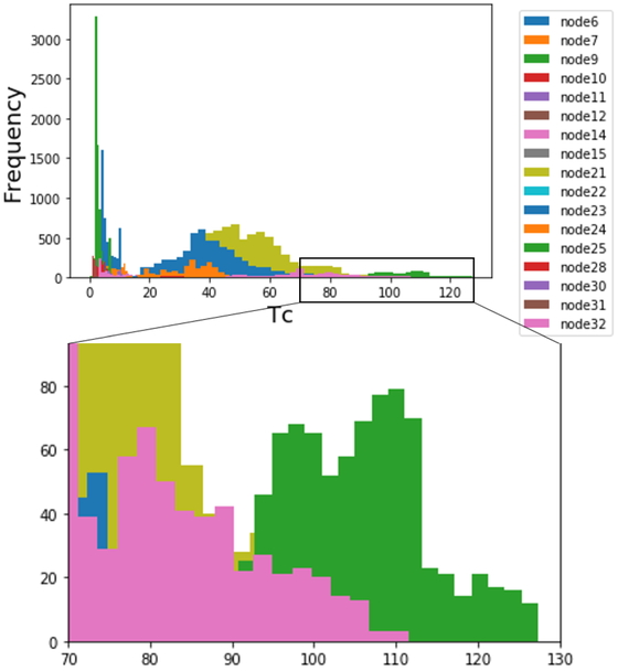
 Predicted T_c for compounds simulated based on T_c dataset.

4 Conclusions

In this study, we proposed and evaluated a method for constructing a model to predict the physical properties of compounds that simultaneously considers both the prediction accuracy and model interpretability. Using the proposed method, which is called DT-RF combining DT and RF, it is possible to elucidate the relationship between the y- and X-variables for the entire dataset based on the visualization of the DT. Furthermore, a more detailed interpretation can be performed based on the importance of X-variables in the local RF models constructed for each terminal node of the DT. Using case studies based on BP, logS, and T_c datasets, the effectiveness of the proposed DT-RF was confirmed, and its precision accuracy and interpretability were evaluated. What can be interpreted in the proposed method is the relationships between y and X. These relationships would be the basis for discussing the processes and the mechanism of expression of properties and activities, and therefore, it is important to prepare appropriate descriptors as X-variables.

The DT-RF method did not exhibit the limitations related to the trade-off between prediction accuracy and model interpretability. In addition, a pseudo-inverse analysis was performed by simulating inorganic compounds that would be suitable as high-performance superconductors. As the predictions made using the DT-RF model are based on the DT method and because the predicted values will lie within the range of y in the training data, the y values predicted with the DT-RF method do not exceed the y-range in training samples. Thus, it would be appropriate for a pseudo-inverse analysis of the proposed DT-RF model not to produce virtual samples exceeding the y-range in training samples but to interpret X-values with a certain Y-value. In addition, the DT-RF model is readily interpretable and should help in the discovery of the underlying mechanisms of different physical properties. However, in some cases, it may be advisable to use a model-construction method that is better suited for extrapolation. In the future, we aim to develop a method for constructing models that exhibit high precision accuracy and interpretability and are suitable for inverse analysis and can predict y values exceeding the y-range in training samples.

Acknowledgements

This work was supported by JSPS KAKENHI Grant Numbers JP19K15352, 20H02553, and 20H04538.

References

• [1]   R. Tibshirani, J. R. Stat. Soc. B, 58, 267 (1996). doi:10.1111/j.2517-6161.1996.tb02080.x
• [2]H. Drucker, C. J. C. Burges, L. Kaufman, A. Smola, V. Vapnik, In Neural Information Processing Systems, 9, 155-161 (1997)
• [3]   C. M. Bishop, Pattern recognition and machine learning; Springer: New York (2006)
• [4]   https://www.oecd.org/chemicalsafety/risk-assessment/37849783.pdf
• [5]   T. Cover, P. Hart, IEEE Trans. Inf. Theory, 13, 21 (1967). doi:10.1109/TIT.1967.1053964
• [6]   D. M. J. Tax, Pattern Recognit. Lett., 20, 1191 (1999). doi:10.1016/S0167-8655(99)00087-2
• [7]   T. Fujita, D. A. Winkler, J. Chem. Inf. Model., 56, 269 (2016). doi:10.1021/acs.jcim.5b00229
• [8]   D. C. Park, M. A. El-Sharkawi, R. J. Marks, L. E. Atlas, M. J. Damborg, IEEE Trans. Power Syst., 6, 442 (1991). doi:10.1109/59.76685
• [9]   S. Kar, J. Roy, D. Leszczynska, J. Leszczynski, Computation (Basel), 5, 2 (2016). doi:10.3390/computation5010002
• [10]   L. Breiman, Mach. Learn., 45, 5 (2001). doi:10.1023/A:1010933404324
• [11]   V. Stanev, C. Oses, A. Gilad Kusne, E. Rodriguez, J. Paglione, S. Curtarolo, I. Takeuchi, npj Comput., Mater., 4, 29 (2018).
• [12]   V. M. Alves, A. Golbraikh, S. J. Capuzzi, K. Liu, J. Chem. Inf. Model., 58, 1214 (2018). doi:10.1021/acs.jcim.8b00124
• [13]   I. M. dos Santos, J. P. G. Agra, T. G. C. de Carvalho, G. L. de Azevedo Maia, E. B. de Alencar Filho, Struct. Chem., 29, 1287 (2018). doi:10.1007/s11224-018-1110-8
• [14]   M. Asahara, R. Fujimaki, IEEE Trans. Parallel Distrib. Syst., 30, 1481 (2019). doi:10.1109/TPDS.2019.2892972
• [15]   R. Eto, R. Fujimaki, S. Morinaga, H. Tamano, PMLR, 33, 238 (2014).
• [16]   Y. Iwasaki, R. Sawada, V. Stanev, M. Ishida, A. Kirihara, Y. Omori, H. Someya, I. Takeuchi, E. Saitoh, S. Yorozu, npj Comput., Mater., 5, 103 (2019).
• [17]   L. Breiman, Mach. Learn., 24, 123 (1996).
• [18]   G. De’ath, K. E. Fabricius, Ecology, 81, 3178 (2000). doi:10.1890/0012-9658(2000)081[3178:CARTAP]2.0.CO;2
• [19]   https://scikit-learn.org/stable/modules/generated/sklearn.tree.DecisionTreeRegressor.html
• [20]   https://scikit-learn.org/stable/modules/generated/sklearn.ensemble.RandomForestRegressor.html
• [21]   https://scikit-learn.org/stable/modules/generated/sklearn.cross_decomposition.PLSRegression.html
• [22]   https://scikit-learn.org/stable/modules/generated/sklearn.svm.SVR.html
• [23]   H. Kaneko, K. Funatsu, Chemom. Intell. Lab. Syst., 142, 64 (2015). doi:10.1016/j.chemolab.2015.01.001
• [24]   P. Filzmoser, B. Liebmann, K. Varmuza, J. Chemometr., 23, 160 (2009). doi:10.1002/cem.1225
• [25]   https://chm.kode-solutions.net/products_dragon.php
• [26]   https://www.rdkit.org/docs/GettingStartedInPython.html
• [27]   J. Bardeen, L. N. Cooper, J. R. Schrieffer, Phys. Rev., 108, 1175 (1957). doi:10.1103/PhysRev.108.1175
• [28]   J. G. Bednorz, K. A. Müller, Z. Phys. B Con., Mat., 64, 189 (1986).
• [29]   Y. Sato, S. Kasahara, H. Murayama, Y. Kasahara, E. G. Moon, T. Nishizaki, T. Loew, J. Porras, B. Keimer, T. Shibauchi, Y. Matsuda, Nat. Phys., 13, 1074 (2017). doi:10.1038/nphys4205
• [30]   https://github.com/parrt/dtreeviz
• [31]   A. Schilling, M. Cantoni, J. D. Guo, H. R. Ott, Nature, 363, 56 (1993). doi:10.1038/363056a0