Article
海難事故を生じた竜巻状渦を発生させたメソβスケール渦のアンサンブル実験

2022 年 100 巻 1 号 p. 141-165

詳細
2022 年 100 巻 1 号 p. 141-165
Ensemble forecasts with 101 members, including one ensemble mean, using ensemble Kalman filter analysis were performed to understand the atmospheric conditions favorable for the development of a meso-β-scale vortex (MBV) that caused shipwrecks as a result of sudden gusty winds in the southwestern part of the Sea of Japan on 1 September 2015. A composite analysis was conducted to reveal the differences in the structure of the MBV and atmospheric conditions around the MBV between the strongest 8 (STRG) and weakest 10 (WEAK) ensemble members. Two of the strongest ten members that developed the MBV much earlier than the other members were excluded from the analysis. The analysis revealed that the near-surface cyclonic horizontal shear to the northeast and the south of the MBV was stronger for STRG than for WEAK. In addition, larger low-level water vapor and its horizontal flux for STRG contribute to greater convective available potential energy to the southeast of the MBV, which results in stronger convection around the MBV. The results of the composite analysis are statistically supported by an ensemble-based sensitivity analysis. Differences in the near-surface horizontal shear were closely related to the structure of the extratropical cyclone in which the MBV was embedded. Although the strength of the extratropical cyclone for STRG was comparable with that for WEAK, the cyclonic horizontal shear of winds in the northeastern quadrant of the extratropical cyclone was greater for STRG than for WEAK.
Between 0300 JST and 0400 JST (Japan Standard Time; UTC + 0900) on 1 September 2015, a sudden gusty wind caused five shipwrecks in the Tsushima Strait (Fig. 1) in the southwestern part of the Sea of Japan, which resulted in five fatalities. Near the locations of the shipwrecks, a meso-β-scale vortex (MBV) with a diameter of about 30 km was observed by the Fukuoka Doppler radar of the Japan Meteorological Agency (JMA). The MBV formed in the northeastern quadrant of a weak extratropical cyclone (EC) that was located west of the Kyushu Islands (Tochimoto et al. 2019; hereafter referred to as T19). Near the location of the MBV formation, warm moist air in the warm sector of the EC intruded from the southeast and contributed to the development and maintenance of active convection. That location was also associated with strong horizontal shear of horizontal wind in the EC (Fig. 10 in T19). T19 performed a triply nested, high-resolution deterministic numerical simulation with a horizontal resolution of 50 m in the innermost domain and suggested that tornado-like vortices that occurred in the west of the MBV center caused the shipwrecks.
There are several types of mesoscale vortex. Mesoscale convective vortices (MCVs), which are associated with quasi-linear convective systems (QLCSs) and mesoscale convective complexes (MCC; Maddox 1980), are often observed in the contiguous United States. MCVs have horizontal scales of 100–300 km (e.g., Davis and Galarneau 2009) and have the strongest vertical vorticity in the mid-troposphere. MCVs usually develop in the stratiform precipitation region associated with QLCSs or preexisting MCCs (e.g., Menard 1989; Raymond and Jiang 1990). Stretching of planetary and relative vorticity is thought to be important for a MCV formation (Weisman and Davis 1998; Yu et al. 1999; Conzemius and Montgomery 2009).
Cyclonic mesoscale vortices forming in the northern end of bow-echo systems are termed “line-end” or “book-end” vortices and originate from horizontal vorticity associated with the vertical shear of environmental winds and/or generated baroclinically (e.g., Davis and Weisman 1994; Weisman and Davis 1998). These vortices have a horizontal scale of 10–100 km and are generally strongest at 2–4 km above ground level (American Meteorological Society 2012). Smaller-scale vortices (mesovortices), which have a horizontal scale of several to tens of kilometers (meso-γ-scale; Orlanski 1975) or smaller (e.g., Boyer and Dahl 2020) and may cause damaging winds, are also observed in QLCSs. Previous studies have demonstrated that tilting of horizontal vorticity in the environment and/or that generated frictionally and baroclinically play a significant role in the formation and development of mesovortices (Trapp and Weisman 2003; Weisman and Trapp 2003; Atkins and St. Laurent 2009; Xu et al. 2015).
The MBV studied by T19 revealed several features that are different from those of MCVs and line-end vortices. It had a horizontal scale of about 30–50 km, and its vorticity was largest near the surface. T19 demonstrated that the source of the strong near-surface vertical vorticity eventually stretched by the updraft of strong convection was environmental horizontal shear between northeasterly, easterly, and southeasterly winds in the EC. With these results in mind, it is hypothesized that the EC had a structure that creates a strong horizontal shear of environments and strong convection in favorable location and timing to intensify the MBV. However, the structure of the EC that caused environments favorable for the development of the MBV has not been fully elucidated.
Ensemble experiments provide a promising approach for examining the predictability of mesoscale disturbances and the environments that are favorable for their occurrence. Melhauser and Zhang (2012) conducted 40-member ensemble experiments and compared the initial conditions and environments between 10 squall-line-forming and 10 non-squall-line-forming ensemble members. They demonstrated that an upper-level trough and a surface low are crucial to the development of the squall line. Ensemble sensitivity analysis (ESA; Ancell and Hakim 2007; Torn and Hakim 2008) has been successfully applied to convective-scale forecasts, although a limited number of ensemble members may inhibit proper identification of important small-scale sensitivity features (e.g., Hill et al. 2016; Wile et al. 2015; Berman et al. 2017). Grunzke and Evans (2017) conducted ensemble experiments to elucidate the predictability and dynamics of a warm-core mesovortex during the “super-derecho” event of 8 May 2009. Using ESA, they demonstrated that the strength of a mesovortex is sensitive to the strength of the upper-level trough, whereby a stronger upper-level trough resulted in a stronger lower-level jet, moisture, and temperature advection, facilitating stronger convection to intensify the mesovortex. Using ensemble experiments with a local ensemble transform Kalman filter (LETKF; Hunt et al. 2007) and ESA, Yokota et al. (2016, 2018) examined the predictability and formation mechanism of a supercell and associated tornado that occurred over Tsukuba, Japan, on 6 May 2012.
In this work, we conducted ensemble experiments using an LETKF to identify the atmospheric conditions favorable for the development of the MBV event on 1 September 2015, which was studied by T19. The remainder of this paper is organized as follows: The methodology is described in Section 2, the results are presented in Section 3, and our findings are summarized and discussed in Section 4.
To predict the MBV probabilistically, we used the NHM–LETKF system (Kunii 2014), in which observations are assimilated with the four-dimensional local ensemble transform Kalman filter (4D-LETKF; Hunt et al. 2004, 2007) based on the forecast error covariance estimated by ensemble forecasts using the JMA non-hydrostatic model (JMANHM; Saito et al. 2006). The JMANHM is a former operational mesoscale prediction model of the JMA and is based on a finite-difference scheme with fully compressible equations, including a map factor. We repeated the forecast-analysis cycles with the JMANHM and the 4D-LETKF to prepare suitable initial states for the probabilistic prediction of MBVs.
We used a doubly nested, 100-member NHM–LETKF with horizontal grid intervals of 15 km and 5 km (hereafter the 15-km and 5-km LETKFs, respectively). The initial and boundary states of the 101 members, including one ensemble mean, of the 15-km LETKF were obtained from the sum of the global forecasts of the JMA and the ensemble perturbations from the 1-week ensemble prediction system of the JMA, whereas those of the 5-km LETKF were from the 100 members of the 15-km LETKF. In both the 15-km and 5-km LETKFs, the number of vertical levels was 50, and the vertical grid interval varied from 40 m near the surface to 886 m near the top of the calculation domain.
In the ensemble forecasts with the JMANHM, we used a hybrid terrain-following vertical coordinate system (Ishida 2007) and adopted a bulk-type singlemoment cloud microphysics scheme that considers mixing ratios of water vapor, cloud water, rain, cloud ice, snow, and graupel (Lin et al. 1983), with modification by Murakami (1990) and Ikawa et al. (1991). Although two-moment schemes are expected to exhibit better performance in representing a feedback process between microphysical processes and other fields, such as convective mass flux, temperature, moisture, and radiation (e.g., Igel et al. 2015), the same model using a one-moment scheme succeeded in nicely reproducing observed features of the MBV in T19. JMANHM also uses the Mellor–Yamada–Nakanishi–Niino (MYNN) level 3 planetary boundary layer scheme (Nakanishi and Niino 2004, 2006, 2009) and a cumulus parameterization based on Kain and Fritsch (1990) and Kain (2004). For the cumulus parameterization, the trigger function of convection, reduction rate of convective available potential energy (CAPE), autoconversion (into precipitation) in the updraft, and time scale of convection were modified to make it suitable for the 5-km horizontal grid interval (Ohmori and Yamada 2004, 2006; Saito et al. 2006, 2007). In the data assimilation with the 4D-LETKF, the relaxation-to-prior spread (Whitaker and Hamill 2012) with an inflation parameter of 0.95 was used to retain sufficient ensemble spread.
The 15-km LETKF assimilated hourly observations in a 3-h assimilation time window in the forecast–analysis cycles starting at 0900 JST on 28 August 2015. The observations included those from surface stations (pressure), radiosondes (horizontal winds, temperature, and relative humidity), aircraft (horizontal winds and temperature), wind profiler radars (horizontal winds), microwave scatterometers (horizontal winds), visible/infrared imagers (atmospheric motion vectors), the Global Navigation Satellite System (precipitable water vapor), and Doppler radar [Doppler velocity and relative humidity estimated from reflectivity (Ikuta and Honda 2011; Ikuta 2012)]. Note that the MBV and surrounding convection are well observed by the radar, which is about 100 km away from the MBV (Fig. 1). These observational data were assimilated to create the mesoscale analysis of the JMA (Honda et al. 2005). The 5-km LETKF, in which 10-min resolution observations (Doppler velocities from the JMA Fukuoka C-band radar and horizontal winds, temperature, and relative humidity from JMA surface stations) were assimilated in 1-h cycles, was started at 1500 JST on 31 August. The calculation procedure and calculation domains are presented in Fig. 2, and the experimental settings are summarized in Table 1.

Observed characteristics of the meso-β-scale vortex on 1 September 2015. (a) Surface weather map at 0300 JST. (b) Radar reflectivity (dBZ) and (c) Doppler velocity (m s−1) observed by the JMA Fukuoka C-band Doppler radar at 0332 JST. The red rectangle in (a) indicates the region in which radar reflectivity and Doppler velocity are presented in (b) and (c), respectively, and the red crosses in (b) and (c) indicate the location of the Fukuoka radar. The solid black circles in (b) and (c) indicate the locations of shipwrecks between 0320 JST and 0335 JST and the open black circles those at around 0355 JST. (Adapted from Fig. 1 in the study by Tochimoto et al. 2019).

(a) Outline of the calculation procedure and (b) the calculation domains of the NHM-LETKF system. The color shading shows the topography in each model (in m). The locations of Tsushima Strait and shipwrecks are indicated by a black rectangle and a red cross, respectively

The 100 members of the 15-km and 5-km LETKFs at 0000 JST on 1 September and their respective ensemble means were used for the initial states of the 6-h extended ensemble forecasts with 101 members (hereafter 15-km EXT and 5-km EXT, respectively). The results of the 5-km EXT forecasts will be discussed in Section 3.
2.2 Classification of simulated MBVs in the ensemble forecastsFigure 3a presents the time sequence of the maximum values of the smoothed vertical vorticity, which is defined by an average of over a 20 × 20-km horizontal square at each grid point at a height of 20 m at 10-min intervals during the period of the experiments, for all members. It should be noted that the simulated MBVs develop about 2 h later than the observed MBV. To plot Fig. 3, we first obtained the maximum values and positions of the smoothed vertical vorticity around Tsushima Strait (33.5–35°N, 128.5–130°E) at 0530 JST, which will be denoted as time T, and their positions were tracked back, whereby the positions of the MBV center at T − 10 min were obtained for a region within a 15 × 15-km area around the MBV center at T. To identify and elucidate the differences in features between ensemble members that produced strong MBVs and those that did not, the strongest 10 members and the weakest 10 members were extracted from all members based on the maximum smoothed vertical vorticity at 0530 JST. The time sequence of the maximum smoothed vertical vorticity for the strongest and weakest 10 members is indicated by the red and blue lines in Fig. 3a. Since 2 of the strongest 10 members (broken red lines in Fig. 3a) developed much earlier than the other 8 members, however, they were excluded from the subsequent analyses. In what follows, the results for the strongest 8 members are denoted as STRG and those for the weakest 10 members as WEAK.

(a) Time series of the maximum vertical vorticity smoothed over a 20 × 20-km2 square at 20-m height. The thick red and thick blue lines depict the members that belong to STRG and WEAK, respectively, and the gray lines indicate the other members. The broken red lines indicate 2 of the strongest 10 members that were excluded from the analyses. (b) Predicted MBV tracks from 0300 JST to 0530 JST. The red and blue lines are the tracks for STRG and WEAK, respectively, and the gray lines are those for other members. The squares and circles indicate the positions of the MBV at 0300 JST and 0530 JST, respectively. The green lines indicate the estimated tracks of the MBV observed by Fukuoka Doppler radar, with green triangles depicting the positions of the MBV at 0230 JST, 0300 JST, 0330 JST, and 0430 JST.
The predicted track of the MBV for each of the 101 ensemble members is presented in Fig. 3b. Most of the predicted MBVs moved northeastward and developed west of Tsushima Island (34–35°N, 128.5–129°E), although radar observations and the deterministic simulation by T19 both revealed that the MBV developed east of Tsushima Island. These differences in tracks are likely due to the locations of EC centers. Figure 4 presents the structures of the EC and MBV for the deterministic simulation (T19) and for a member of the ensemble simulation (the 53rd member, #53). Here, #53 is selected because it reproduces the second-strongest MBV, which is located closer to the average location of the MBV for STRG than the strongest MBV reproduced by #66. The centers of the EC in the ensemble experiments (Fig. 4b) tend to be located more westward than that in the deterministic simulation in T19 (e.g., Figs. 4b) and in the objective analysis data (not shown). Although MBVs for STRG also tend to be located slightly northward (∼ 10 km on average) and eastward (∼ 30 km on average) than those for WEAK, the difference is not pronounced. To elucidate the impact of Tsushima Island on the MBV, we conducted additional experiments in which Tsushima Island was removed and replaced by sea, confirming that Tsushima Island hardly affects the development of the MBV (not shown). The EC structure and its associated horizontal wind fields near the surface are reasonably similar between T19 and the ensemble member #53 (Figs. 4a, b). The overall structures of the simulated MBV in the deterministic and ensemble simulations (Figs. 4c, d, respectively) are also reasonably similar to the observations (Figs. 1b, c), although the coarse horizontal resolution of the model is not able to reproduce the detailed characteristics of the observations. Strong reflectivity and large amounts of rainwater are found to the west and northwest of the center of the MBV, both in the observations and in the simulations. The vertical structure of the MBV reproduced by the ensemble simulation is also reasonably similar to that reproduced in T19 (Figs. 4e, f), in that the vertical vorticity is strongest near the surface and is confined to a height lower than 3.5 km in both the ensemble and deterministic simulations. Although other STRG ensemble members are not presented, they have similar structures to those of #53. Thus, the ensemble simulations reasonably reproduce the overall structures of the MBV.

(a) Horizontal distribution of vertical vorticity (color shading; s−1) and horizontal wind vectors (arrows; m s−1) at 20-m height at 0420 JST (mature stage of the simulated MBV) in T19. (b) As in (a), but for ensemble experiment #53 at 0530 JST. (c) Expanded view of the horizontal distribution of rainwater mixing ratio (color shading) and vertical vorticity (contour lines; s−1) at 20-m height in a simulation with 2-km horizontal resolution at 0420 JST in T19 for the area indicated by a square in (a). (d) As in (c), but for ensemble experiment #53 at 0530 JST for the area indicated by a square in (b). (e) A vertical cross-section of the vertical vorticity simulated in T19 along A-A′ in (c). (f) As in (e), but for ensemble experiment #53 along B-B′ in (d).
The predicted vertical vorticity at 20-m height at 0530 JST on 1 September 2015 for each member of STRG and WEAK is presented in Fig. 5. The vertical vorticity is noticeably larger for STRG than for WEAK: the maximum vorticity is approximately 3 × 10⁻³ s−1 for STRG and approximately 2 × 10⁻³ s−1 for WEAK.
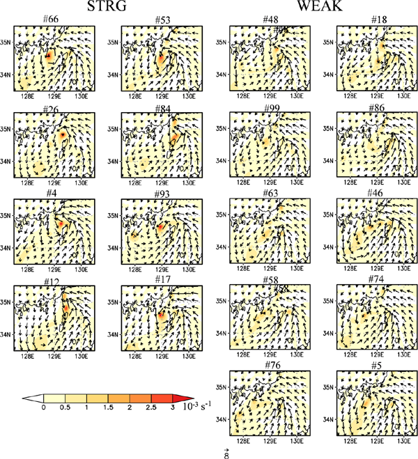
Vertical vorticity (color shading; 10−3 s−1) and horizontal wind vectors (arrows; m s−1) for 8 members of STRG (left 2 columns) and 10 members of WEAK (right 2 columns) at 20-m height at 0530 JST.
Figure 6 presents the time–height cross-section of maxima of the vertical vorticity and vertical velocity, which are smoothed over an area of 20 × 20 km at each height for STRG and WEAK. STRG members show near-surface development of the vertical vorticity from 0400 JST to 0530 JST after its intensification above 1-km height between 0130 JST and 0400 JST. As proposed by T19, an upward perturbation pressure gradient force associated with the intensified vertical vorticity above 1 km is likely to have contributed to an acceleration of updrafts (e.g., Markowski and Richardson 2010; Nielsen and Schumacher 2018). In contrast, none of the WEAK members exhibited rapid intensification of the near-surface vertical vorticity.

Time-height cross-section of the maxima of the vertical vorticity (color shading; s−1) and updraft (contour lines; m s−1) both smoothed over a 20 × 20-km horizontal square centered on the MBV at each height for STRG (left 2 columns) and WEAK (right 2 columns).
The rapid intensification of the near-surface vertical vorticity in STRG members between 0330 JST and 0530 JST was accompanied by strong meso-β-scale updrafts (Fig. 6). For WEAK MBVs, 7 of 10 members (#18, #86, #63, #46, #58, #74, #76) have notably weaker updrafts than STRG between 0030 JST and 0300 JST (Fig. 6). A role of the strong updrafts at the early development will be examined in the later section in more detail. Although the other 3 of 10 WEAK members (#48, #99, and #5) had strong meso-β scale updrafts between 0000 JST and 0530 JST, near-surface vertical vorticity did not develop. Thus, it is suggested that strong convection alone is not sufficient to explain the observed intensification of the MBV. The intensification process of the near-surface vertical vorticity will be addressed in the next section.
3.2 Composite analysis a. Composite Analysis with respect to the MBV centerWe conducted a composite analysis to examine the structure and development process of the MBV and its meso-β-scale environment surrounding the MBV. Physical variables were superposed with respect to the MBV center, as defined in Section 2.1. In this study, key-time (KT) is defined based on a 10-min interval output as the time when the growth rate of the smoothed vertical relative vorticity (ζ) during a 20-min interval [i.e., (ζt + 10min − ζt − 10min)/20min] is a maximum. The composite analysis was conducted every 1 h from KT minus 3.5 h (KT − 3.5 h) to KT plus 0.5 h (KT + 0.5 h).
Figure 7 presents the time–height cross-section of the vertical vorticity and vertical velocity, where these variables are averaged over 30 × 30-km2 horizontal square around the MBV to examine the evolution of the MBV-scale fields. Between KT – 3.5 and KT – 2.5 h, the vertical vorticity for STRG gradually develops in the layer between near the surface and 2500-m height, whereas that for WEAK gradually decreases (Figs. 7a–c). In this period, although the vertical vorticity for STRG is comparable to WEAK, the updraft for STRG is remarkably stronger than that for WEAK (Figs. 7d–f). The vertical vorticity for STRG becomes larger than that for WEAK between KT – 2.5 h and KT – 1.5 h, and then the vertical vorticity for STRG rapidly develops between KT – 1.5 h and KT, eventually exceeding 1.0 × 10⁻³ s−1 at KT. On the other hand, the vertical vorticity for WEAK only slightly develops, reaching 0.6 × 10⁻³ s−1, which is notably smaller than that for STRG. After KT – 1.5 h, updrafts above 1000-m height for STRG are slightly weaker than those for WEAK, whereas those below 1000-m height are comparable between STRG and WEAK.

Time-height cross-section of vertical vorticity averaged over a 30 × 30-km horizontal square (color shading; 10−3 s−1) around the MBV center for (a) STRG and (b) WEAK. (c) Difference in the smoothed vertical vorticity (s−1) between STRG and WEAK. (d) and (e) are the same as (a) and (b), except for updraft (contour lines; m s−1) averaged over a 30 × 30-km horizontal square around the MBV center at each height. (f) Difference in the averaged updraft (m s−1) between STRG and WEAK.
To elucidate the differences in the physical processes for the development of the MBV between STRG and WEAK, we also examined terms in the vertical vorticity equation, which may be written as follows:
 |
Figure 8 presents the time–height cross-section of stretching and tilting terms, where these terms at each height were averaged over 30 × 30-km square around the MBV center. Between KT − 3.5 h and KT + 0.5 h, the stretching term for STRG is noticeably larger than that for WEAK (Figs. 8a–c). Thus, larger stretching of the vertical vorticity results in stronger MBV. The contribution of tilting is slightly larger for STRG than for WEAK, though the contribution is much smaller than that for stretching for both groups (Figs. 8d–f). Between KT − 3.5 h and KT − 2.5 h, the updrafts for STRG are stronger than those for WEAK and contribute to larger stretching since the vertical vorticity of the MBV in this period is comparable between STRG and WEAK (Figs. 7a–c). Between KT − 2.5 h and KT − 1.5 h, both stronger updrafts and larger vertical vorticity for STRG compared with those for WEAK contribute to the larger stretching term. Then, between KT − 1.5 h and KT + 0.5 h, larger vertical vorticity near the surface for STRG still likely contributes to the larger stretching since the updrafts for STRG and WEAK are comparable (Figs. 7d–f).

Time-height cross-section of the stretching term averaged over a 30 × 30-km2 horizontal square (10−6 s−2) around the MBV center for (a) STRG and (b) WEAK. (c) Diff erence in the stretching (10−6 s−2) between STRG and WEAK. (d) and (e) are the same as (a) and (b), except for the tilting term (10−6 s−2) averaged over a 30 × 30-km horizontal square at each height. (f) Diff erence in the tilting term (10−6 s−2) between STRG and WEAK.
Horizontal distributions of vertical velocities at 500-m height (Figs. 9a, b) show that updrafts with a horizontal scale of 30–50 km in the eastern and northeastern quadrants of the MBV at KT − 3 h for STRG are stronger than those for WEAK (Figs. 9a, b). Between KT − 3 h and KT − 1.5 h, the updrafts around the MBV strengthen. The difference between STRG and WEAK becomes more pronounced at KT − 1.5 h, whereby the maximum updraft exceeds 0.9 m s−1 for STRG, and the region in which updrafts exceed 0.2 m s−1 (meso-β-scale) for STRG is wider than that for WEAK (Figs. 9c, d). Thus, stronger updrafts with a horizontal scale of 30–50 km for STRG likely caused larger stretching, which resulted in stronger MBV. The difference in the maximum updraft, which is located in the northeast quadrant of the MBV center, however, becomes less pronounced at KT in both groups (Figs. 9e, f).

Composite field of the vertical velocity at 500-m height (color shading; m s−1) and vertical vorticity at 20-m height (contour line with 0.0025 s−1 interval) at KT − 3 h for (a) STRG and (b) WEAK. (c) and (d) are the same as (a) and (b), respectively, but at KT − 1.5 h JST. (e) and (f) are the same as (a) and (b), respectively, but at KT. The origin (0, 0) indicates the location of the MBV center.
Now, we investigate how environmental factors influence the larger stretching of the vertical vorticity for STRG, resulting in rapid strengthening of the MBV. Figures 10a–c presents composite fields of water vapor mixing ratio and water vapor flux at 100-m height. At KT − 3 h, a belt-shaped region of the low-level vapor mixing ratio exceeding 18 g kg−1 extends from the southeast to the east of the MBV center for STRG (Fig. 10a). The water vapor mixing ratio to the south and southeast of the MBV for STRG is at least 1.2 g kg−1 greater than that for WEAK (Figs. 10b, c). Moreover, the northward and eastward low-level water vapor flux in the southeast of the MBV for STRG has stronger convergence around the MBV.

Composite fields of water vapor mixing ratio (color shading; g kg−1), temperature (blue contour lines; K), and water vapor flux (arrows; g kg−1 m s−1) at 100-m height at KT − 3 h for (a) STRG and (b) WEAK. (c) Difference in water vapor mixing ratio (color shading; g kg−1) and water vapor flux (arrows; g kg−1 m s−1) between STRG and WEAK. Composite fields of CAPE (J kg−1) at KT − 3 h for (d) STRG and (e) WEAK. (f) Difference in CAPE (J kg−1) between STRG and WEAK. (g)–(i) are the same as (d)–(f) except for SHR6 (m s−1). The origin (0, 0) indicates the location of the MBV center.
Composite fields of temperature also show some diff erences between STRG and WEAK (Figs. 10a–c). A region of higher temperatures for STRG is present in the region to the southeast of the MBV center at KT − 3 h (Fig. 10a). The difference in the temperature between STRG and WEAK is about 0.6–1.2 K (Fig. 10c). The above results indicate that larger water vapor mixing ratio, its flux, and warmer temperature create unstable stratification that is a favorable condition for strong convection for STRG (Figs. 9a–d). Therefore, the difference in CAPE (Moncrieff and Millar 1976) between STRG and WEAK are examined (Figs. 10d–f). The CAPE for STRG to the southeast of the MBV is larger than that for WEAK: the values of CAPE for STRG are about 600–800 J kg−1, whereas those for WEAK are 500–600 J kg−1. Thus, the environment of the MBV for STRG has more potential for stronger convection than that for WEAK.
Since the vertical shear of horizontal wind generally acts to support the organization of convective storms (e.g., Weisman and Klemp 1982), composite fields of the vertical shear between 20 m and 6000 m (SHR6) are also compared between STRG and WEAK (Figs. 10g–i). Although SHR6 for both STRG and WEAK exceeds 18 m s−1 in the northwest and east of the MBV, SHR6 for STRG is larger than that for WEAK. Thus, the vertical shear for STRG is more favorable for organizing convective system than that for WEAK.
After this time, both the MBV and updrafts associated with convection for STRG become stronger than those for WEAK (Fig. 7). Thus, positive feedback between strong convection and the development of the MBV is likely to have occurred (e.g., Nielsen and Schumacher 2016): Strong convection leads to the intensification of the MBV through the stretching of the vertical vorticity. The intensified MBV induces strong low-level winds, resulting in persistent strong water vapor flux and its convergence around the MBV (Figs. 10, 11), and thus leads to the development and maintenance of the convection (e.g, Figs. 7, 8), which in turn intensifies the MBV. It is noted that no strong cold pool for STRG exists (Fig. 10a), so that cold pool processes do not seem to contribute to the development of the convection.

Composite fields of vertical vorticity (color shading; 10−4 s−1) and horizontal wind vectors (arrows; m s−1) at 20-m height at KT − 3 h for (a) STRG and (b) WEAK. (c) Difference in the vertical vorticity (color shading; 10−4 s−1) and horizontal wind (arrows; m s−1). (d), (e), and (f) are the same as (a), (b), (c), respectively, but at KT – 1.5 h. The dashed black and green boxes indicate the regions where the vertical vorticity and horizontal convergence for STRG are stronger than those for WEAK.
Next, we examine the wind fields in the environments around the MBV. Figure 11 presents composite fields of the vertical vorticity and wind fields at 20-m height at KT − 3 h and KT. At KT − 3 h, for both STRG and WEAK, southwesterly and southerly winds converge in the region to the south and southeast of the MBV and reach the MBV center. In the region to the northeast of the MBV center, there is a region with cyclonic horizontal shear between southeasterly and easterly winds. The differences in the vertical vorticity and wind fields between STRG and WEAK at KT − 3 h are presented in Fig. 11c. Winds south of the MBV center (in the region indicated by the dashed green box in Fig. 11c) have a larger westerly component, and the vertical vorticity is larger for STRG. In contrast, to the north of the MBV center (in the region indicated by the dashed black box in Fig. 11c), stronger northeasterly winds to the north, stronger southerly wind to the south, and associated larger vertical vorticity due to cyclonic horizontal shear are found for STRG. Since these differences are found outside a radius of 15 km around the MBV center and the cyclonic rotation within a radius of 15 km around the MBV is comparable between STRG and WEAK at this time (Figs. 7a–c), the differences in cyclonic horizontal shear of winds between STRG and WEAK are not related to the strength of the MBV. Moreover, since the MBV has not fully developed at KT − 3 h, the structure of the MBV is not likely to contribute to the difference in wind fields around the MBV. Thus, the environmental vertical vorticity associated with horizontal shear, which is capable of being stretched later by updrafts, exists outside the MBV circulation for STRG. The center of the MBV moves northward into the region of cyclonic horizontal shear. At KT – 1.5 h, the vertical vorticity at the center of the MBV for STRG further increases to 0.0024 s−1 (Fig. 11d), whereas for WEAK, it is about 0.0017 s−1 (Fig. 11e). The STRG members continue to show larger horizontal wind shear in the northeast of the MBV (in the region indicated by the dashed black box in Fig. 11f) than the WEAK members. The characteristic of the horizontal shear is similar to that in T19 (cf. Fig. 10 in T19).
Besides the cyclonically rotational wind field corresponding to the MBV, there exists another cyclonic rotational wind field, which corresponds to the center of the EC, to the west of the MBV (∼ x = −100 km). The distance between the centers of the EC and the MBV is larger for STRG than for WEAK. The vertical vorticity associated with the EC between KT − 3 h and KT is stronger for STRG than for WEAK (Figs. 11c, f). The relationship between the strengths of the EC and MBV will be discussed later in Section 3c.
b. Composite analysis with respect to the center of the extratropical cycloneTo investigate the relationship between the EC structure and the MBV development, we conducted a composite analysis in which physical variables were superposed with respect to the center of the EC. The composite analysis was conducted for the ensemble initial time of the ensemble experiment (0000 JST, hereafter “INIT”) and KT – 3 h. Figure 12 presents the composite fields of the vertical vorticity, horizontal divergence, and horizontal wind at 20-m height for STRG and WEAK, as well as the difference fields between the STRG and WEAK composites, at INIT and KT – 3 h. It should be noted that these variables were smoothed by taking an average over an 80 × 80-km horizontal square to focus on the structure of the EC. At INIT, the convergence of horizontal wind to the southeast of the EC center (x = 80–120 km, y = −50 km to 0 km; the dashed purple box in Fig. 12) for STRG is stronger than that for WEAK. In this region, the smoothed vertical vorticity associated with the horizontal shear of wind for STRG is slightly larger than that for WEAK (Figs. 12a–c). These characteristics are also found at 500-m height (not shown). At KT − 3 h, a region of larger vertical vorticity for STRG becomes more evident in a region east of the EC center (x = 50–100 km, y = −50 km to 50 km; the dashed purple boxes in Figs. 12d–f). The difference in the vertical vorticity between STRG and WEAK in this region is 0.2–0.6 × 10⁻⁴ s−1. The meso-β-scale vertical vorticity of the MBV is comparable between STRG and WEAK at this time (Figs. 7a–c), whereas the horizontal scale of the region where there is a notable difference in the vertical vorticity between STRG and WEAK is about 100–150 km, which is larger than that of the MBV embedded in this region (Fig. 12f). Thus, it is suggested that stronger vertical vorticity associated with the environmental horizontal shear outside the radius of 15 km around the MBV is likely to have played an important role in the development of the MBV.
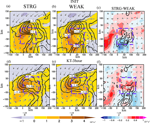
Composite fields of vertical vorticity (color shading; 10−4 s−1), horizontal divergence (contour lines; 10−4 s−1), and horizontal wind (arrows; m s−1) at 20-m height at INIT (0000 JST), for (a) STRG and (b) WEAK, and (c) their differences. Note that variables are smoothed over an 80 × 80-km horizontal square, and contour lines indicate values with an interval of 0.2 × 10⁻⁴ s−1. (d)–(f) are the same as (a)–(c), respectively, but at KT − 3 h. The origin (0, 0) indicates the location of the EC center. The dashed purple boxes indicate the regions where the vertical vorticity associated with MBV develops.
To understand why the cyclonic vertical vorticity associated with the environmental horizontal shear for STRG became stronger than that for WEAK, we examined the differences in the stretching and tilting terms of the vertical vorticity at 500-m height at KT − 3.5 h (Fig. 13). The stretching that is attributed to horizontal convergence with a horizontal scale of 100–150 km east of the EC center (dashed purple boxes in Figs. 13a, b) for STRG is notably larger than that for WEAK. Although tilting for STRG in the same region positively contributes to the intensification of the vertical vorticity and is larger than that for WEAK, the values of tilting are notably smaller than those of stretching. Thus, the large stretching term caused by horizontal convergence for STRG mainly contributes to the generation of cyclonic horizontal shear with a horizontal scale of 100–150 km.

Composite fields of the stretching term at 500-m height (color shading; 10−8 s−2) and horizontal wind (arrows; m s−1) at 20-m height at KT − 3.5 h, for (a) STRG and (b) WEAK, and (c) their differences. Note that variables are smoothed over an 80 × 80-km horizontal square. (d)–(f) are the same as (a)–(c) except for the tilting term (10−8 s−2). The origin (0, 0) indicates the location of the EC center. The dashed purple boxes indicate the regions where the vertical vorticity associated with MBV develops.
To understand why the horizontal convergence for STRG is stronger than that for WEAK, we also examined the differences in low-level equivalent potential temperature and horizontal structure of precipitation system around the EC between STRG and WEAK (Fig. 14). At INIT, there is stronger convergence of horizontal wind for STRG in the region of x = 50–120 km, y = −50 km to 0 km (Figs. 12a–c; the purple dashed box in Figs. 14a–c). Further to the southwest (x = 0–50 km, y = −150 km to −50 km; the purple box in Figs. 14a–c), the low-level equivalent potential temperature is higher, and the southerly winds are stronger for STRG, indicating a larger transport of warm moist air to the north. At KT − 3 h, the differences in the convergence of horizontal wind and rainwater mixing ratio between STRG and WEAK (Figs. 12d–f, 14d–f) become larger, indicating stronger precipitation system with a horizontal scale of 100–150 km for STRG (x = 0–150 km, y = −50 km to 100 km; the purple dashed boxes in Figs. 14d–f). In a region to the south (x = 0–150 km, y = −150 km to −50 km; the purple boxes in Figs. 14d–f), higher equivalent potential temperatures and stronger southerly winds continue to occur for STRG, which indicates that stronger advection of low-level warm moist air contributed to the intensification and maintenance of the convection system. These results suggest that a stronger precipitation system with a horizontal scale of 100–150 km caused by stronger convergence of warm moist air intensified the environmental vertical vorticity associated with horizontal shear of winds, resulting in a favorable condition for the MBV development.

As in Fig. 13, but for equivalent potential temperature at 100-m height (color shading; K) smoothed over an 80 × 80-km horizontal square and rainwater mixing ratio (green contour lines; g kg−1) at 500-m height. The dashed purple boxes indicate the regions where the vertical vorticity associated with MBV develops. The solid purple boxes indicate the regions where there are differences in the south and southwesterly winds and equivalent potential temperature.
To further explore the sensitivity of the MBV development to physical variables in the environment, we conducted an ESA (Ancell and Hakim 2007; Torn and Hakim 2008). We examined the sensitivity of the maximum vertical vorticity smoothed over a 20 × 20-km2 horizontal area at 20-m height (ζmax20m, j) to the variable xij at each grid point i (i = 1, … N):
 |
First, we examine the sensitivity of the MBV vorticity to thermodynamic variables. Sensitivities to low-level specific humidity, water vapor flux, and temperature at KT − 3 h are presented in Figs. 15a, b. The smoothed vorticity of the MBV has a positive sensitivity to low-level water vapor and temperature in the south of the MBV center (Figs. 15a, b). The correlation coefficient between the vertical vorticity of the MBV and low-level water vapor (temperature) in this region is statistically significant at the 95 % confidence level. In the same region, the vorticity of the MBV is also sensitive to northward water vapor flux (vectors in Figs. 15a, b). Moreover, the vorticity of the MBV has a positive sensitivity to CAPE to the south and southeast of the MBV center and to SHR6 to the east and northeast of the MBV center (Figs. 15c, d). These results indicate that the MBV strength is associated with strong convection, which is organized by the large vertical shear of horizontal wind and unstable stratification created by the increase in low-level water vapor, its flux, and temperature.

Sensitivity of vertical vorticity to (a) water vapor mixing ratio at 100-m height, (b) temperature at 100-m height at KT − 3 h, (c) CAPE, and (d) SHR6. The contour lines indicate the standard deviations of (a) water vapor mixing ratio, (b) potential temperature, (c) CAPE, and (d) SHR6. The vectors in (a) and (b) indicate the sensitivity of vertical vorticity to the moisture vapor flux at 100-m height. The white dots indicate the regions where the correlation coefficient is statistically significant at the 95 % confidence level.
The sensitivity of the smoothed vorticity of the MBV to the horizontal wind components at 20-m height at KT − 3 h and KT − 1.5 h is presented in Fig. 16. The sensitivity to westerly and southerly winds is high in the regions to the south and southeast of the MBV (within the dashed green box). In this region, the correlation coefficients are statistically significant at the 95 % confidence level. In the region to the northeast of the MBV center (in the region indicated by the dashed black box in Fig. 16), the sensitivity to northerly and easterly winds with a statistically significant correlation (at the 95 % confidence level) is observed, although the difference in the strength of the MBV between STRG and WEAK is fairly small. Note that this region lies outside of the MBV, the diameter of which is 30 km. At KT − 1.5 h, the regions with high sensitivity to horizontal winds continue to exist to the south, north, and northeast of the MBV center. Thus, the strength of cyclonic horizontal shear in these regions is considered to contribute to this particular MBV.

Sensitivity of vertical vorticity at the MBV center to (a) meridional winds and (b) zonal winds at 20-m height at 0330 JST. The contours in (a) and (b) indicate the standard deviation of meridional and zonal winds, respectively. (c) and (d) are the same as (a) and (b), respectively, but at KT − 1.5 h. The vectors indicate the sensitivity of vertical vorticity to the wind field. The white dots indicate the regions where the correlation coefficient is statistically significant at the 95 % confidence level. The dashed black and green boxes indicate the regions where the sensitivity to meridional and zonal winds is high.
The sensitivity of the smoothed vorticity to the horizontal wind components also shows that the strength of the MBV is sensitive to a cyclonic circulation of the EC, which is located to the southwest of the MBV center (x = −150 km to −60 km, y = −50 km to 60 km; Fig. 16) at KT − 3 h and KT − 1.5 h. Thus, the development of the MBV might be sensitive to the strength of the EC. To examine the relationship between the strength of the EC and that of the MBV, scatter plots of the EC circulation at INIT and KT − 3 h, calculated over a 100 × 100-km square centered on the EC, and the circulation of the MBV calculated over a 20 × 20-km square centered on the MBV at 0530 JST are presented in Fig. 17. The calculated EC circulation does not include the vorticity in the northeastern periphery of the MBV. The EC center was determined by the location of the maximum vertical vorticity smoothed using an 80 × 80-km2 square horizontal average at 100-m height. It turned out that there is no significant correlation between the strength of the EC and that of the MBV: the correlation coefficients at KT − 3 h and KT − 1.5 h are 0.13 and −0.06, respectively. These results indicate that the strength of the EC was not strongly related to the strength/development of the MBV.

Scatter diagram of the circulation of the MBV (106 m2 s−1) calculated over a 20 × 20-km2 horizontal square centered on the MBV at 20-m height and circulation (106 m2 s−1) calculated over a 100 × 100-km2 horizontal square centered on the EC at 20-m height.
Figure 18 presents the distribution of the EC center with respect to the MBV center at KT − 1.5 h for each ensemble member, along with the composite field of horizontal wind for all members. The EC centers for STRG are concentrated near the location of the composite cyclonic circulation center of the EC (x = −10 km, y = −10 km), whereas those for WEAK are more widely scattered. Members that do not belong to STRG or WEAK but have MBVs with relatively large maximum vertical vorticity at 0530 JST also tend to exist close to the EC center for STRG. This explains why composite fields for STRG and WEAK show that the vertical vorticity associated with the EC for STRG is notably stronger than that for WEAK (Fig. 13).

Distribution of the EC center with respect to the MBV center for STRG and WEAK ensemble members at KT − 1.5 h. The yellow to red color shading indicates the maximum vertical vorticity (10−4 s−1) of the MBV at a height of 20 m and smoothed over a 20 × 20-km2 horizontal square at 0530 JST. The green and blue circles indicate the locations of the EC center for STRG and WEAK, respectively. The origin (0, 0) indicates the location of the MBV center. The arrows indicate the composite horizontal wind field (m s−1) for all ensemble members.
Ensemble experiments with 101 members using an LETKF were conducted to elucidate favorable environments and important factors for the development of a meso-β-scale vortex (MBV). In the ensemble experiments, the MBV formed in the northeast quadrant of the EC and had a structure similar to those of the observations and the deterministic simulation (T19). The majority of ensemble members, however, reproduced an MBV to the west of Tsushima Island, whereas the observed MBV actually occurred to the east of Tsushima Island. Note that Tsushima Island did not affect the present results according to a sensitivity experiment, in which the island was eliminated and was changed to a sea surface.
A schematic diagram of the MBV development is presented in Fig. 19. The strong convergence of low-level southerly winds with warm moist air in the EC for STRG intensifies the convection with a horizontal scale of 30–50 km, resulting in the early development of the MBV. The fact that the MBV for STRG has stronger updrafts with a horizontal scale of 30–50 km suggests that the transport and convergence of warm moist air from the south and southeast resulted in stronger convection, which in turn caused larger stretching of the vertical vorticity. Stronger convergence of warm and moist air in the EC for STRG also results in stronger precipitation system with a horizontal scale of 100–150 km. The strong convergence associated with this precipitation system for STRG causes the large cyclonic horizontal shear in the warm sector during the early stage of the MBV development. The identification of the importance of low-level moisture in the development of mesoscale convective systems is similar to the findings of previous studies (e.g., Schumacher 2015; Kato 2018).

Schematic diagram of the MBV development.
At the later developing stage, the large cyclonic horizontal shear in the environment around the MBV is suggested to contribute to the intensification of the MBV through the stretching of its vertical vorticity. These results are also statistically supported by an ESA, which shows that the development of the MBV is strongly correlated with environmental cyclonic horizontal shear outside the radius of the MBV. It is likely that a positive feedback between the horizontal shear and MBV also played an important role in the development of the MBV after the initial development of the MBV. During the continued development phase of the MBV, the region of large horizontal shear for STRG moves northward, and the MBV is situated in the northeastern quadrant of the EC.
Although the structure of the EC, which has a large horizontal shear in the warm sector region, is shown to be crucial to the development of the MBV, what causes the different structure of the EC among ensemble members has not yet been elucidated. To investigate this issue, an ensemble experiment for examining the effects of the synoptic-scale environment on the structure of the EC that favors the development of the MBV might be useful. Moreover, the resolution of the ensemble experiments in the present study was not sufficiently high to simulate the tornado-like vortices, such as those reproduced in the deterministic simulation of T19. Thus, an ESA using ensemble experiments with a high-resolution model that are capable of reproducing tornado-like vortices is desired to examine the detailed dynamics and predictability of the tornado-like vortices.
Since the code of the JMA Nonhydrostatic model and local ensemble transformed Kalman filter system is owned by JMA, we need to ask JMA for permission on the basis of individual request.
The authors grateful to Dr. Masayuki Kawashima and two anonymous reviewers for their constructive comments that significantly improved our original manuscript. This work was supported by JSPS KAKENHI Grants 18H01277 and FLAGSHIP2020 of the Ministry of Education, Culture, Sports, and Technology within the priority study Advancement of Meteorological and Global Environmental Predictions Utilizing Observational “Big Data” (Project ID: hp160229, hp170246, hp180194, hp190156). This study was also supported by MEXT as “Program for Promoting Researches on the Supercomputer Fugaku” (Large Ensemble Atmospheric and Environmental Prediction for Disaster Prevention and Mitigation; Project ID: hp200128, hp210166) and by the Cooperative Program (159, 2021) of Atmosphere and Ocean Research Institute, The University of Tokyo.
Since the code of the JMA Nonhydrostatic model and local ensemble transformed Kalman filter system is owned by JMA, we need to ask JMA for permission on the basis of individual request.