Abstract
The near-real-time merged satellite and in-situ data global daily sea surface temperature (SST) of the Japan Meteorological Agency (hereinafter abbreviated as R-MGD) is subjected to filtering out short-time-scale fluctuations from observations prior to the analysis time. Therefore, the rapid SST change due to the passage of tropical cyclones (TCs) is thought to cause biases. Here, the biases in the R-MGD with respect to in-situ observations were quantified along the passage of TCs in the western North Pacific. First, we examined a case study on the approach of three successive TCs in August–September 2020. The R-MGD had positive biases of > 2°C just after the passage of three TCs, and negative biases were observed after one week of the last TC's passage. The comparison of the R-MGD with a moored buoy indicates that the biases can be explained by short-term fluctuations filtered out and the SST prior to the analysis time in R-MGD analysis. Second, the composite analysis from May 2015–October 2020 indicates that the statistically significant biases at the observation points ranged between −1 days and +4 days for positive biases and between +7 days and +14 days for negative biases relative to the time of the closest approach of a TC within 500 km. The positive SST bias is largely associated with cold subsurface water and intense TCs, being pronounced in the mid-latitude, except around the Kuroshio and Kuroshio extension regions. The assimilation of in-situ observations recorded within 72 h prior to the R-MGD analysis time through additional optimal interpolation alleviates these biases because this process redeems short-time-scale fluctuations. The impact on TC forecasts and the validity of the optimal interpolation experiment against the independent observations were also investigated.
1. Introduction
The quality of near-real-time daily sea surface temperature (SST) analysis is important for weather prediction, oceanic prediction, oceanic ecosystems, and fishery activities. In terms of disaster prevention and mitigation, the improvement of near-real-time SST analysis can contribute to enhancing weather forecasting because severe weather events such as heavy rainfall events and tropical cyclones (TCs) are sensitive to SST (Emanuel 1986; Iizuka and Nakamura 2019; Ito and Ichikawa 2021; Kusunoki and Mizuta 2008; Manda et al. 2014; Moteki and Manda 2013; Nayak and Takemi 2019; Tsuguti and Kato 2014).
Currently, the Japan Meteorological Agency (JMA) creates several SST analysis products. Daily SSTs in the global ocean are objectively analyzed in a near-real-time and delayed mode, called the merged satellite and in-situ data Global Daily SST (MGDSST; Japan Meteorological Agency 2019; Kurihara et al. 2006). Meanwhile, the JMA has also conducted another SST analysis for climate monitoring known as COBE-SST (Ishii et al. 2005), along with High-resolution merged satellite and in-situ data SST (HIMSST; https://ds.data.jma.go.jp/gmd/goos/data/pub/JMA-product/him_sst_pac_D/Readme_him_sst_pac_D). Among MGDSST, COBE-SST, and HIMSST, the near-real-time version of MGDSST (referred to as R-MGD in this study) uses preprocessed satellite and in-situ observations from 17 days before the analysis time. The R-MGD has been used as the boundary condition for simulations, with an atmospheric global spectral model (GSM), and as the “observations” that are assimilated in the ocean data assimilation system used for the global model and North Pacific model (Hirose et al. 2019; Japan Meteorological Agency 2017, 2021; Sakamoto et al. 2019). Although the boundary condition of the operational mesoscale model has been HIMSST since March 2019 (https://www.jma.go.jp/jma/kishou/books/nwptext/52/No52_all.pdf), the R-MGD can indirectly influence their skills through the lateral boundary condition. Therefore, the R-MGD is very important for weather and ocean predictions and ocean monitoring as the near-real-time information. Although the R-MGD utilizes the observations available prior to the analysis time, JMA also performed the delayed-mode analysis of MGDSST (referred to as D-MGD in this study) by utilizing observations within 10 days before and after the analysis time. D-MGD is not available for weather and ocean forecasts, but it provides a more reliable SST field for research purposes and climate studies.
The procedure for generating the R-MGD carried out by JMA (as of December 11, 2020) is briefly summarized in Fig. 1 (Kurihara et al. 2006; personal communication, JMA Office of Marine Prediction). Firstly, quality control and preprocessing are applied. For example, it has been known that SSTs obtained from the Advanced Very High-Resolution Radiometer have systematic biases due to aerosols and clouds (Huang et al. 2015; Zhang et al. 2004). The biases are adjusted based on the match-up to the statistics of buoys. After quality control and preprocessing, five types of Gaussian filtering in space and time are applied to the SST anomaly data (with respect to climatology) obtained from satellite infrared sensors and microwave sensors having weight w. The weight is determined using the following equation:
Here,
σx and
σy are the zonal and meridional filtering scales in km, respectively,
σt is the temporal filtering scale in day, and
dx (in km),
dy (in km), and
dt (in day) represent the corresponding distances between the analysis and observation points. As for temporal filtering, two filters
days and
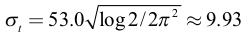
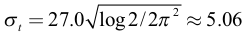
days are used. They are conventionally referred to as “27-day filter” and “53-day filter”, respectively, because the output power spectrum becomes halved for a sufficiently long input dataset
1. After Gaussian filtering, the long and large scale of the SST anomaly field was adjusted to the long and large scale of in-situ observations, as carried out by
Reynolds and Smith (1994) and
Reynolds et al. (2002). Finally, they were merged using optimal interpolation (OI) (
Fig. 1).
The strategy of R-MGD analysis to use a time-filtered dataset for daily analysis is understandable considering the large inertia of the ocean and insufficient amount of data. If we do not apply temporal filtering nor prepare a background field, it is difficult to avoid unphysical SST structures, such as sharp changes and missing values. Nevertheless, it should be noted that the actual rapid SST changes in the last few days are substantially dropped from the R-MGD because of the rather long-time-scale temporal filtering. Such an example is SST cooling and SST recovery occurring in a short-time scale caused by the passages of TCs (Dare and McBride 2011; Price et al. 2008).
In general, SST is affected by air-sea fluxes, including radiation, entrainment, and detrainment of water at the base of the ocean mixed layer (OML) through vertical mixing, vertical transport, and horizontal transport. Commonly, although solar heating at daytime warms and stabilizes the upper ocean, winds enhance the ocean turbulence that mixes the water vertically and wind-induced circulation plays an important role in SST distribution (Price et al. 1986). As for the passage of TCs, winds can cause the SST to decrease mainly because of the one-dimensional vertical mixing and three-dimensional upwelling processes (Price 1981; Shay 2010; Yablonsky and Ginis 2009). The one-dimensional vertical mixing process is related to the storm-induced current in the OML. The diff erence in horizontal currents serving as a vertical shear becomes strong across the base of the OML, satisfying the critical Richardson number. Thus, the cold water underneath is entrained into the OML. The OML increases in thickness, and the waters become colder. This process is pronounced on the right-rear side of the TC center position primarily because the wind stress vector turns clockwise in resonance with the near-inertial motion slightly enhanced by the asymmetric distribution of wind fi eld (Price 1981). Thus, the region of large SST decrease is parallel to TC motion. In addition to this vertical one-dimensional process, cyclonic wind forcing transports the upper ocean water horizontally away from the TC center. This surface transport induces an upwelling near the TC center. As a result, cold water is transported to the upper ocean in a three-dimensional manner. Although vertical mixing is generally a primary mechanism in SST cooling, a strong upwelling becomes dominant for a very slow-moving cyclone (Kanada et al. 2021; Yablonsky and Ginis 2009). After the passage of TCs, the restratifi cation of the upper ocean requires approximately one month, in which a rapid SST increase is seen in the fi rst two weeks, as examined by Mei and Pasquero (2012). Their study suggested that the increasing net radiation inputs speed up SST recovery, in which baroclinic instability plays an important role in the structure of the ocean temperature. The composite analysis of the SST from Argo data in the western North Pacifi c shows that the SST decrease starts one day prior to the passage of a TC (Wu and Chen 2012) and that three-quarters of SST decrease recover in 15 days (Lin et al. 2017).
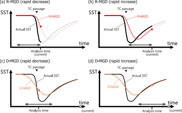
Both the one-dimensional and three-dimensional SST cooling processes are relevant to the time scale of the inverse of the Coriolis parameter, f−1, and the SST increases in several weeks during the recovery process. Because the temporal fi ltering in the R-MGD and D-MGD analyses overlooks the short-term SST changes, a part of the actual SST change can be discarded. In particular, the R-MGD only refl ects the observed SSTs in the past with respect to the analysis time. When a high SST dropped in a short-timescale, the R-MGD partly inherits the high SST according to the weight in Eq. (1) (Fig. 2a). Positive SST biases are expected to be large when the SST decrease is large, with cold water present just below the sea surface and the occurrence of strong and slow-moving TCs. The negative SST biases in the R-MGD may appear also during the SST recovery stage if the SST increase is rather fast (Fig. 2b).
Therefore, the fi rst aim of this work is to describe the SST biases in the R-MGD with respect to the TC passage based on a case study and composite analysis. The second aim is to propose a method for alleviating these biases by utilizing the in-situ observations obtained just before the SST analysis time. The remainder of this paper is organized as follows. In Section 2, we explain the data and methodology used for the study. Section 3 exemplifies the SST biases in the R-MGD caused by the passage of three TCs during August–September 2020. Composite analysis of the SST biases in the R-MGD for the period of May 2015–October 2020 is presented in Section 4. This section also reveals the physical background of the large SST biases. In Section 5, we demonstrate that the additional OI of the in-situ observations (within 72 h prior to the R-MGD analysis time) can alleviate the SST biases. In Section 6, we conducted numerical experiments with the JMA nonhydrostatic model (JMA-NHM) to show the impact of updated SST on the TC forecasts. In Section 7, we discuss the validity of the OI experiment against independent observations. Finally, our conclusions are summarized in Section 8. Additional results for the other basins and products are described in Supplements 1–6. For example, the negative and positive SST biases are, respectively, expected in D-MGD before and after the analysis time (Figs. 2c, d), and Supplement 1 describes the biases of D-MGD.
2. Data and method
The successive passages of TCs Bavi, Maysak, and Haishen during August–September 2020 were used as a case study to exemplify the biases in the R-MGD. The composite analysis from May 2015 to October 2020 (66 months) within the target region of 100–180°E and 0–60°N was performed (detailed in Section 4), which corresponds to the region responsible for the Regional Specialized Meteorological Center Tokyo (RSMC Tokyo). In this paper, we focus on the western North Pacific because the analysis of tropical cyclone intensity and genesis is conducted by a different agency in each basin and because JMA high-quality daily ocean temperature is available during this period for the western North Pacific. We briefly discuss the global SST biases caused by TC passages in Supplement 2.
The R-MGD is the daily SST dataset of the global ocean on a grid of 0.25° × 0.25° every day (Japan Meteorological Agency 2019; Kurihara et al. 2006). The preprocessed SST data obtained from each satellite infrared or microwave sensor were subjected to five types of filters (Fig. 1), and the long and largescale filtered component was adjusted by in-situ SST observations. The data from each filter and each satellite were finally merged through OI. The R-MGD at day m refers to the value averaged from 1800 UTC on day m-1 to 1800 UTC on day m (personal communication, JMA). Note that weather forecasts based on JMA's GSM (also referred to as JMA-GSM), with an initial time of 1800 UTC on day m and 0000 UTC, 0600 UTC, and 1200 UTC on day m+1, employ the R-MGD on day m. We also used the D-MGD in later sections. The climatological mean SST refers to the mean value of D-MGD between 1984 and 2014. Currently, the D-MGD is available only until December 2019.

In-situ observations were taken from in-situ SST Quality monitoring (i Quam) developed at NOAA (Xu and Ignatov 2014) (available at https://www.star.nesdis.noaa.gov/socd/sst/iquam/data.html; accessed on November 19, 2020). The i Quam is a globally compiled in-situ SST dataset obtained from ships, drifters, moored buoys, and Argo floats having a quality control (QC) flag. The QC processes comprised preprocessing (resolving duplicates from multiple transmission or dataset merging), plausibility/geolocation, internal consistency, external consistency, and mutual consistency checks. On the basis of these tests, a quality flag is appended to each observation [Table 7 of Xu and Ignatov (2014)]. For reliability, we used only the data with the QC flag of “best quality” and did not use the data having “acceptable quality” and “low quality” unless otherwise noted. Note that neglecting the “acceptable quality” and “low-quality” data may lead to some underestimation of the SST biases, as we shall see in Section 3 and Supplement 3. We used only one randomly sampled datum of the day from one platform for the composite analysis in Section 4 when two or more data were available.
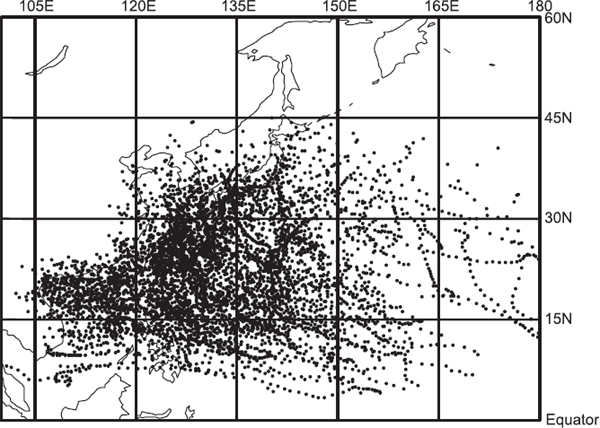
The TC center position and intensity were taken from the best track of RSMC Tokyo (https://www.jma.go.jp/jma/jma-eng/jma-center/rsmc-hp-pub-eg/besttrack.html). The best track data are not considered before a TC reaches the threshold of tropical storm status or an extratropical cyclone subjected to transition from the TC. TC translation speed was simply calculated from the difference in the TC's center positions in the next 6 h. Figure 3 shows the 6-hourly center positions of 153 TCs used for the composite analysis.
We stratified the data according to the difference in prestorm ocean temperature between 50 m and 1 m (δT50), TC maximum wind speed, and TC translation speed. The oceanic data are given by the JMA-Meteorological Research Institute (MRI) Multivariate Ocean Variational Estimation system (MOVE; Japan Meteorological Agency 2019; Usui et al. 2006, 2017), in which the base physical model is the MRI Community Ocean Model (Tsujino et al. 2017). Because a high-resolution four-dimensional variational data assimilation system did not cover the entire target region for the period of interest, we used daily outputs having a horizontal grid spacing of 0.5° obtained from a three-dimensional variational data assimilation system for the North Pacific Ocean. Note that the R-MGD was assimilated into the operational ocean model as the “observations” into the MOVE system. Large negative values of δT50 represent very cold water at 50 m relative to the surface water. We also used the satellite-based SST from the Global Change Observation Mission 1st-Water (GCOM-W1) Advanced Microwave Scanning Radiometer 2 (AMSR2) onboard the GCOM-W1 satellite. It is a remote sensing instrument for measuring microwave emission from the surface. Here, we employed the L3 standard product that has a horizontal grid spacing of 0.25° (available at https://gportal.jaxa.jp/gpr/?lang=en).
The gridded analysis data are linearly interpolated in space to compare them with in-situ observations. As for temporal interpolation, we simply calculated the difference between an in-situ observation from 1800 UTC on day m-1 to 1800 UTC on day m and the corresponding R-MGD on day m. For presentation purposes, we refer 1800 UTC at day m as the R-MGD analysis time. Although the daily mean of the MOVE refers to the value averaged from 0000 UTC on day m to 0000 UTC on day m+1, the infl uence of the time lag of 6 h was at most 0.1°C in terms of the composite mean SST bias and was thus, negligible.
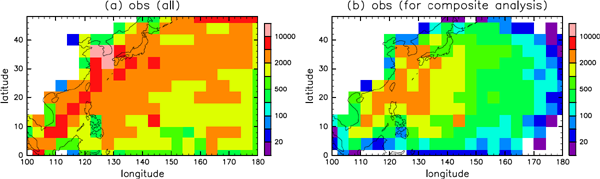
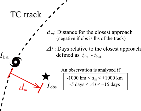
We categorized the SST bias data according to the relative time and location with respect to the TCs. This was achieved by employing the TC's closest approach distance to an in-situ observation, dm, and the observation time relative to the time of the closest approach, Δt = tobs − tbst (Fig. 4). For a given observation at the observed time tobs, we first seek the TC center position at time tbst that exhibited the closest approach within 1000 km from the observation point while satisfying −5 days < Δt < +15 days. According to previous studies, TC-induced SST cooling starts from one day prior to TC passage and three-quarters of the SST cooling are recovered in 15 days after the TC passage (Lin et al. 2017). Therefore, the period of −5 days < Δt < +15 days is suffi cient to quantify SST biases in background, rapidly decreasing, and rapidly increasing stages. Although weak TC-induced SST anomalies may persist for more than 15 days (Lin et al. 2017; Mei and Pasquero 2012), we did not analyze the data beyond 15 days because they are too long to elucidate the infl uence of the TC. As for the relative position of an observation, the positive dm is defi ned as the closest approach distance when the observation is on the right-hand side of the direction of the TC motion, whereas the negative dm indicates the observation on the left-hand side. Note that dm almost corresponds to the cross-track distance (perpendicular to the TC motion direction) from the observation point to the TC's closest approach point, as shown in Fig. 4. It reveals when the SST bias appears and how long it persists after the TC's closest approach. If the TC center position was not recorded within 1000 km from the observation point during the target period, the observation was not used in the composite analysis. If more than one TC approached the observation point, only the TC with the smallest |dm| was analyzed. The total number of available in-situ observations with the best-quality fl ag is approximately 9.1 × 10⁶ from May 2015 to October 2020 in 100°E–180° and 0–60°N. Sampling only one data point from the same platform on one day yielded 5.7 × 10⁵ observations (Fig. 5a), and we used 1.4 × 10⁵ observations for the composite analysis to evaluate the infl uence of the TC passages (Fig. 5b). In addition to the coordinates spanned by dm and Δt, we used the so-called TC-centered coordinate that looks down the direction of the TC motion as an ordinate axis, and the TC center position is located at the origin of the coordinate. In this coordinate, the abscissa and ordinate axes correspond to the cross-track and along-track distances, respectively.
In fact, the mean biases discussed in the later sections are slightly different between the ships and other observation platforms by approximately 0.05–0.10 K (average: 0.07 K) within |dm| < 500 km, consistent with the statistics of Xu and Ignatov (2014). We neglect this difference because it is much smaller than the TC-induced biases. We are not sure regarding the reason for this, but it can result from a ship-based observation deployed in a shallow level on average2 or the influence of the engine of a ship.
3. Case study in August–September 2020
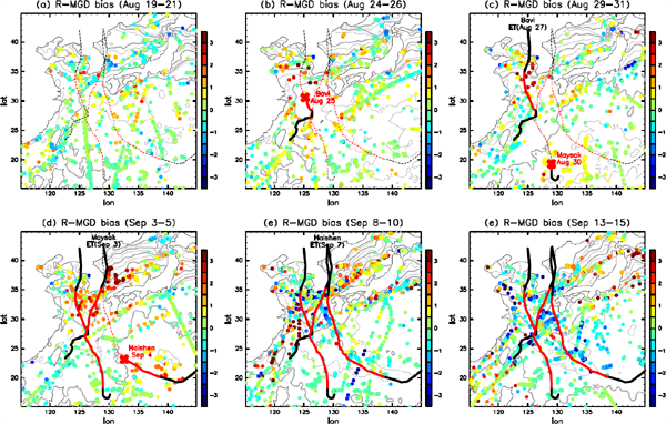
From August 23, 2020, to September 7, 2020, TCs Bavi, Maysak, and Haishen successively passed around the East China Sea, Yellow Sea, and Japan Sea. According to the RSMC Tokyo best track, the lifetime maximum wind speeds of these TCs were 85, 95, and 105 kt, respectively. All TCs exhibited a maximum wind speed of 85 kt or more over the East China Sea or Yellow Sea. Here, we exemplify the SST biases in the R-MGD along the passage of these TCs. Figure 6 shows that the SSTs were over 30°C in the eastern part of the East China Sea, which was much higher than the climatological SST during the prestorm period on August 20. At that moment, the SST biases in the R-MGD were relatively small, except for some negative biases along the east and south coasts of the Korean Peninsula (Fig. 6a). The SST biases tended to become positive around +1°C along the track of Bavi (Fig. 6b). On August 29–31, the positive SST bias reached +2–3°C after a few days in the Yellow Sea in a wake of Bavi and +0.5°C to the east of the Philippines around the center of TC Maysak (Fig. 6c). It is also notable that a negative SST bias appears along the track of Bavi in the south of East China Sea. Figure 6d shows that the SST biases in the R-MGD were around +2°C in the East China Sea and Yellow Sea. The positive SST biases of more than +3°C were also remarkable in the southwestern part of the Sea of Japan (Fig. 6d). Although the SSTs in the R-MGD decreased by 2–4°C in the Yellow Sea and East China Sea along the passages of TCs Bavi and Maysak in two weeks until September 4, a comparison with the in-situ data shows that the SST decrease in the R-MGD was still insufficient to represent the actual SST drop. On September 4, a positive SST bias in the right rear of the track of TC Haishen was also observed. After Haishen's transition to an extratropical cyclone, negative biases less than −1.5°C continued in existence for more than one week in the East China Sea, Yellow Sea, and western part of the Sea of Japan (Figs. 6e, f). To sum up the observations, the positive SST biases in the R-MGD emerged for several days along the TC track, whereas the negative SST biases appeared after approximately one week and continued for another week.
These characteristics of the R-MGD were also seen in the SSTs from GCOM-W1 AMSR2. Figures 7a, b show that the SST dramatically decreased according to the passage of three TCs. However, the magnitude of decrease is exceedingly weak in the R-MGD, particularly just after the passage of TC Haishen (Fig. 7b). AMSR2 SST indicates an increase in SST as a recovery after the passage of TCs such as in 134–145°E and 18–30°N (Fig. 7c). By contrast, the R-MGD remains cold relative to AMSR2 SST.

We compared the R-MGD at 126.03°E and 33.08°N with the observations made by the coastal moored buoy ID 22107 at Marado operated by Korean Meteorological Agency (KMA), including the non-“best-quality” ones (Fig. 8). The buoy-based SST substantially dropped from 30.1°C to 24.5°C in only four days (August 23–27), and it decreased from 28.9°C (August 25) to 25.4°C (August 26) in one day. This is consistent with the passage of TC Bavi that approached this region on August 25–26. After the passage of Bavi, the buoy-based SST increased toward the climatological mean SST and became 26.3°C on August 30. However, on the successive approaches of TCs Maysak and Haishen, the buoy-based SST decreased again and remained around 24°C until September 8. After the passage of the three TCs, in the middle of September, the buoy-based SST increased toward the climatological mean SST.
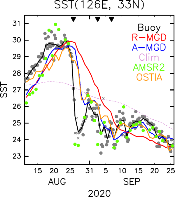
In contrast to the rapid change in the moored buoy, the temporal change in the R-MGD was exceedingly gentle. This led to a large overestimation of the SST in the R-MGD on and just after the passage of the TCs. An SST bias of more than +1°C was continually observed from August 25 to September 5, and the maximum SST bias reached +4.8°C on August 27. It is also notable that the restoration of the SST toward the climatological value (at the end of August and in the middle of September) was not seen in the R-MGD. This causes the negative SST bias to be approximately −1°C in mid-September. By contrast, the SST bias was positive at the end of August presumably because a very gentle decrease in the R-MGD was insufficient to catch up the dramatic decrease in the moored buoy. In addition, the passage of TC Maysak further decreased the SST at that moment. In fact, the dramatic decrease in the SST was obvious by the AMSR2 product at the nearest grid point. This implies that the SST biases in the R-MGD were well captured by, at least, some satellite observations, but the temporal filtering that uses the “27-day” scale or more and the availability of the data in the near-real-time prevent the rapid SST decrease in the R-MGD analysis. We also show the time-series in Operational Sea Surface Temperature and Sea Ice Analysis (OSTIA), which is the near-real-time version of SST analysis operationally conducted by the United Kingdom Meteorological Office (Donlon et al. 2012). The bias in OSTIA is smaller than that in the R-MGD for the rapid SST decrease and increase. OSTIA is expected to better capture short-term SST changes because the main analysis process employs a previous analysis field as a first guess field and digests the observations within a 36-h assimilation window through an OI approach (Donlon et al. 2012).
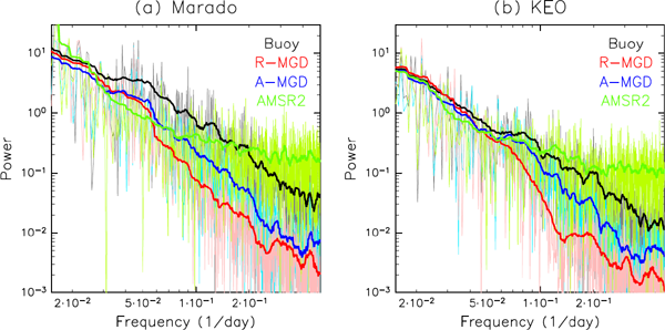
Figure 9a shows the power spectrum of the SST anomaly (relative to the daily climatology) from July 2015 to June 2020 for this moored buoy. The power of the high-frequency mode was largely suppressed in the R-MGD analysis as expected from the temporal smoothing. The power of the R-MGD is half for a period of < 20 days and only one-tenth for a period of < 5 days. It suggests that the TC-induced rapid SST change in a few days is hardly reproduced in the R-MGD analysis. By contrast, the power for a period of a few days was much stronger in GCOM-W1/AMSR2 than in the moored buoy probably due to the nature of the polar orbital satellite that estimated the SST from snapshots. To ensure the characteristics of the R-MGD, we investigated the SST change in the Kuroshio extension region. The suppression of the high-frequency component was also seen in the moored buoy at Kuroshio Extension Observatory (KEO; 32.3°N and 144.6°E) (Fig. 9b). The power of the R-MGD is half for a period of < 15 days and only one-tenth for a period of < 8 days.
4. Composite analysis
Figure 10a shows the composite bias of the R-MGD with respect to the in-situ observations in a dm-Δt coordinate for all cases. The positive bias of the R-MGD in −0.5 day < Δt < 3.5 days is statistically significant, with a confidence level of 95 %, as found using a twosided t-test. The region of the statistically significant positive biases ranges around 500 km on each side. In other words, the positive SST bias, with a bandwidth of several hundred kilometers, persists for a few days along the TC path. The mean positive bias between −150 km < dm < 250 km in −0.5 day < Δt < 3.5 days was +0.40°C. The maximum positive value of +0.52°C was observed at dm = 0 km and Δt = 2 day. The bias tended to be large at the center and on the right-hand side of the TC track. This presumably corresponds to the shear-induced SST decrease along the TC passage (Ito et al. 2015; Price 1981; Price et al. 1994). Another notable feature of Fig. 10a is that the negative SST bias peaked at a value of −0.29°C in 7.5–13.5 days after the passage of the TCs. It represents that the restoration of the SST toward the climatological mean value was not captured in the R-MGD analysis, as exemplified at Marado in the mid-September of 2020 (Fig. 8). In terms of forecasts, a detrimental impact can last for at least a couple of weeks after the TC passage. In a TC-centered coordinate, a statistically significant SST bias was found between 200 km ahead of the TC center and 700 km behind the TC center (Fig. 10b). We can ensure that the positive bias was larger at the center and on the right-hand side of the TC track.

According to previous studies (Lin et al. 2008; Yablonsky and Ginis 2009), the TC-induced SST decrease depends on the upper ocean thermal structure, TC intensity, and translation speed of the TC. Because large SST decreases are likely to incur a large SST bias in the R-MGD, we stratified the SST biases according to the deviation of ocean temperature at 50-m depth, with respect to the ocean temperature at 1 m, at Δt = −3 days both obtained from MOVE (δT50), maximum wind speed at the closest approach (Vmax), and TC translation speed at the closest approach (U). Figures 11a–c show the composite mean of three groups stratified according to δT50. The thresholds of each group were determined to approximately contain the same number of samples. The SST bias is much larger when the ocean temperature at 50 m is much cooler than the sea surface (Figs. 11a–c). This result is consistent with the fact that a large SST decrease is expected with cold water just beneath the surface. The positive bias reached up to +1.16°C near the TC center three days behind the closest approach of a TC. The SST bias was also large when the maximum wind speed Vmax was strong (Figs. 11d–f). It seems a little surprising that relatively large positive biases are associated with the fast-moving TCs (Figs. 11g–i) because slow-moving TCs generally induce a large SST decrease due to persistent wind (Lin et al. 2008; Price 1981; Yablonsky and Ginis 2009). This can be explained by the spurious correlation, as shown later with Fig. 12.

Figure 11 shows that the duration of the positive biases and negative biases was not dependent on the classification according to δT50, Vmax, and U, except in cases with very cold subsurface water of δT50 < −4.0°C. When δT50 < −4.0°C, positive SST biases lasted slightly longer, and negative biases were weak (Fig. 11c). This was presumably because the R-MGD analysis requires relatively long time to catch up the dramatic decrease of the actual SST as exemplified in the end of August after the passage of TC Bavi (Fig. 8).
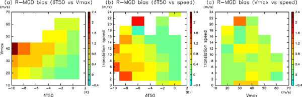
It is likely that three parameters (δT50, Vmax, and U) are correlated in the western North Pacific. Slow-moving TCs are frequently seen in low-latitude areas where the depth of the OML is much deeper. To avoid the influence of spurious correlation on the magnitude of positive SST bias, we calculated the composite mean of the SST bias for observations during −150 km < dm < 250 km and −0.5 day < Δt < 3.5 days (Fig. 12). Figure 12a clearly shows that the positive bias strongly depends on δT50 and Vmax. The composite mean bias reached as much as +2.23°C at δT50 < −10°C and Vmax = 40 m s−1. This indicates that we should be aware of the large SST positive bias in the R-MGD around +2°C, with a width of several hundred kilometers during several days, when a strong TC passes over the region of shallow OML with very cold subsurface water. The positive SST biases tend to be large with slow-moving TCs for a given δT50 (Fig. 12b). Therefore, the relatively large SST biases, with fast-moving TCs in Fig. 11g, are merely an artifact due to the fast-moving TCs that tend to appear where δT50 is strongly negative. The only exception was the strongly positive bias at U = 21 m s−1 and δT50 = −6°C. The relevant observations were deployed in 148–152°E and 37–40°N when TC Sanvu headed north in 2017. It was rare that a TC still had the Vmax of 65 kt at this latitude, and it caused the large biases.
The multiple linear regression model yields the coefficients as shown below:
This analysis indicates that the positive SST biases highly depend on δ
T50, and
Vmax and
U are also relevant parameters.
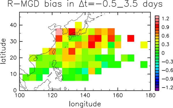
For practical applications, it is useful to describe the geographical distribution of SST biases along the TC passage. Figure 13a shows that the composite mean SST bias for observations during −150 km < dm < 250 km and −0.5 day < Δt < 3.5 days generally increases with increasing latitude, except the region along the Kuroshio current. The composite mean SST bias is approximately +1°C in the northern part of the East China Sea, Yellow Sea, and Sea of Japan. Positive biases are also notable along the line between 130°E, 24°N, and 156°E, 36°N. This geographical distribution can be explained by the climatological features of δT50. The large positive SST biases in the East China Sea, Yellow Sea, and Sea of Japan correspond to the cold subsurface water in these regions, where a large SST bias is expected because of a TC easily affecting the SST along its passage. The weak stratification around the Kuroshio and Kuroshio extension regions can explain the relatively weak positive bias near Okinawan Islands and in the south and east of mainland Japan. By contrast, the composite mean SST bias is relatively small in the south of 20°N.
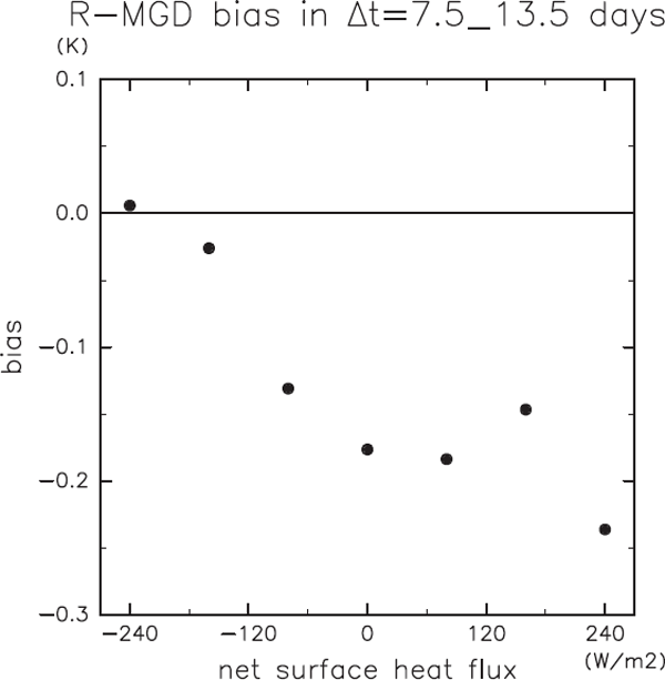
The composite mean SST bias for observations in −350 km < dm < 350 km and 7.5 days < Δt < 13.5 days is generally negative (Fig. 10a). Figure 14 shows the composite mean SST bias for observations during −350 km < dm < 350 km and 7.5 days < Δt < 13.5 days, stratified according to the net surface heat fluxes averaged over 5 days prior to the observation taken from the Japanese 55-year Reanalysis (Kobayashi et al. 2015). It indicates that the negative SST bias over a wake of the TC passage is more pronounced when the net heat flux from the atmosphere to the ocean is large. It is reasonable because the recovery of SST is rapid in such a case.
5. Bias correction by additional OI
As demonstrated in Sections 3 and 4, the R-MGD contains TC-related biases lasting for at least two weeks after the TC approach. One potential issue is that short-term fluctuations are mostly removed in current data processing (Figs. 1, 8, 9). There are potential candidates to consider the short-term fluctuations in the R-MGD analysis using in-situ observations, data assimilation, and high-frequency satellite-derived products. As a trial experiment, we conducted a simple additional OI of in-situ observations that were obtained within 72 h before the R-MGD analysis time. Because in-situ observations are currently used only for adjusting longer than “53-day” scale and large structures of satellite-derived SST estimates, the incorporation of in-situ observations within the mentioned 72 h is a potential way to incorporate the short-timescale fluctuations of the SST fields into R-MGD analysis.
In our additional OI process, the R-MGD was regarded as the first guess field, and the in-situ observations within 72 h before the R-MGD analysis time were regarded as the observations. The target region of OI was set the same as in the previous sections. The basic equation for OI is represented as follows:
where
xa is the updated analysis field (hereafter referred to as A-MGD),
xb is the first guess field representing the R-MGD,
y refers to the in-situ observations,
B is the background error covariance matrix,
H is an observation operator, and
R is an observation error covariance matrix. Here, an element of the background error covariance,
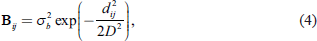
Bij, is assumed to be a simple function of the distance between two locations as follows:
where
σ2b is the magnitude of the background error covariance,
dij is the distance between the two locations, and
D is the influence radius.
R =
σ2oI is a diagonal matrix. Because deviations from the reference values are relatively large in ship-based observations (
Xu and Ignatov 2014), we employed different magnitudes of observation errors for ship-based observations alone (
σ2o, ship) and for the others (
σ2o, other). Note that from
Eqs. (3) and
(4), it is obvious that the analysis increment
xa −
xb depends on the ratio of
σo/
σb, rather than
σo and
σb themselves.
For the analysis on day m, we first created a single super-observation (sum of the background value and the averaged innovations in a certain size of region and time) by taking an average of misfits between the in-situ observations and R-MGD in a 1° by 1° bin from 1800 UTC on day m-3 to 1800 UTC on day m. Here, we considered all best-quality in-situ observations regardless of the existence of TCs around the observations. Although we analyzed only one observation for the same platform on one day in Section 4, here we utilized all observations having the “best-quality” flag. The current additional OI is computationally inexpensive and only takes a few seconds to create the SST analysis at day m with one CPU of AMD EPYC™ 7601.
To reduce the TC-induced biases, we performed a sensitivity test to search for an optimal combination of σo, ship/σb, σo, other/σb, and D by fitting the analysis value to the independent observations that satisfy −500 km < dm < 500 km and −2 days < Δt < 5 days during 2012–2014. For evaluation purposes, observations from 75 % of the randomly selected platforms were used for the additional OI. Observations from the remaining platforms were reserved as independent observations, which were not used for the additional OI. Then, we conducted the additional OI for all combinations of σo, ship/σb, σo, other/σb, and D as shown in Table 1. The smallest root mean square error of the analysis against the independent observations was achieved when σo, ship/σb = 1.6, σo, other/σb = 1.0, and D = 300 km. Thus, we employ these values to construct A-MGD during 2015–2020.
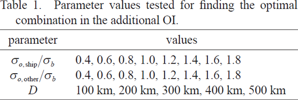
Figure 15a shows the analysis increment (A-MGD minus R-MGD) on September 4, 2020, overlapped by dots indicating the SST biases in the R-MGD used for OI, and Figs. 15b, c show the SST fields of the R-MGD and A-MGD on the same day. The analysis increment generally has an opposite sign to the biases in the R-MGD (Fig. 15a), indicating that the additional OI process successfully tried to compensate for the biases. Comparing A-MGD and R-MGD, the SST in A-MGD was found to be lower in the East China Sea, Yellow Sea, Sea of Japan and around the track of TC Haishen and higher in the South China Sea.

We compared the A-MGD with the R-MGD at the location of the coastal moored buoy, as shown in Fig. 8. Although we did not use non-“best-quality data” on August 27 in the additional OI process, the rapid SST drop was better reproduced in A-MGD than in the R-MGD. In addition, the restoration of the SST in the middle of September was reproduced well in A-MGD. In terms of the power spectrum over five years, A-MGD gained more power in the period < 20 days. Its spectrum data were closer to the spectrum of the moored buoys (Fig. 9).
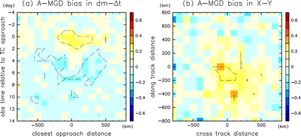
Figure 16a shows the composite bias of the A-MGD with respect to the in-situ observations in a dm-Δt coordinate, as shown in Fig. 10. The mean bias was substantially reduced over two weeks after the passage of TCs. The maximum positive bias was 0.24°C, and the negative bias was −0.17°C, which is much smaller than those in Fig. 10a. The decrease in the bias is also obvious in a TC-centered coordinate system (Fig. 16b). Therefore, this approach can diminish the SST biases associated with the TC passage.
As indicated by the reasoning in the present section, the quality of SST analysis can be improved using a simple additional OI easily built upon the existing system with a tiny computational cost. Of course, the current system can be further improved by more appropriate treatment of error covariances, diurnal variation particularly due to clear-sky insolation in a weak wind condition, further quality controls, use of satellite-based short-term fluctuations, and smaller grid spacings. For example, although the influence radius was set at a constant value of 300 km, the dynamic horizontal scale should be adjusted around the coastal region and western boundary currents. The observation error standard deviation σo should be dependent on the type of platform and number of observations used for a single super-observation. They are left for future studies. Nevertheless, the current experiment clearly shows that utilizing the in-situ observations within 72 h before the R-MGD analysis time can enhance the representation of the SST field, particularly for short-time scale fluctuations that were mostly removed in the current R-MGD analysis. In addition, we would like to remind that the basic SST structure originally and stability of the system embedded in the R-MGD were not destroyed by this process. This OI merely adds an analysis increment whose scale is determined by the background error covariances and observation density.
6. Weather forecast experiment
6.1 Experimental setting
To quantify the impact of updated SST fields on TC forecasts, we conducted a set of 5-day simulations with the R-MGD and A-MGD using the JMA-NHM (Saito 2012; Saito et al. 2006). The JMA-NHM uses a horizontally explicit and vertically implicit scheme as a dynamical core, with six-category bulk microphysics (Ikawa and Saito 1991), a modified Kain–Fritsch convective scheme (Kain and Fritsch 1990), a clear-sky radiation scheme (Yabu et al. 2005), and a cloud radiation scheme (Kitagawa 2000). Boundary layer turbulence is determined by the Mellor–Yamada–Nakanishi–Niino level-3 closure model (Nakanishi and Niino 2004). The initial and boundary conditions were given by forecasts of the GSM of JMA.
The domain was discretized into 1001 × 1001 grid points centered at 130°E and 30°N. We employed the Lambert conformal projection with grid spacings of 5 km. There were 35 vertical layers, with the model top of 22 km. The time step was 20 s. Our 5-day simulations were conducted once a day when there is a TC at the initial time of 1200 UTC from May 2020 to October 2020. We employed the R-MGD and A-MGD as the bottom boundary condition, and SSTs were fixed during the run.
We used the methodology by Sakai and Yamaguchi (2005) to track the position of TCs from the 6-hourly outputs, in which the TC's center position was defined as the location of the minimum sea-level pressure (MSLP). Tracking started when a storm was started to be recorded as a TC in the records of RSMC Tokyo best track data. Forecast accuracy was not verified before a storm reaches the threshold of tropical storm status or an extratropical cyclone subjected to transition from the TC. Once the storm experienced the extratropical transition, the tracking was terminated.
6.2 Results
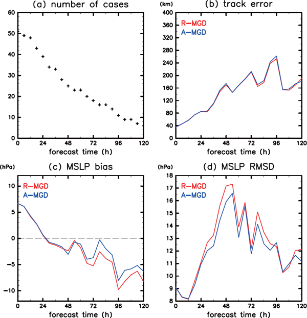
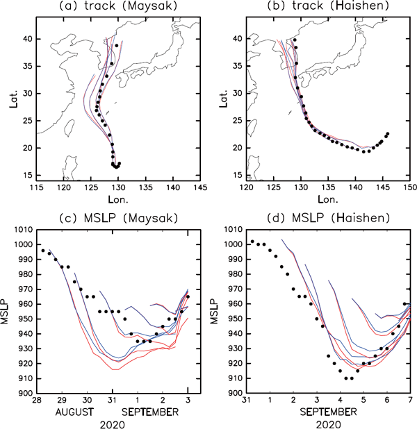
We first investigate the forecasts of TC Maysak and Haishen in 2020, which illustrates the influence of SST biases due to the passage of TCs (Fig. 6). Figures 17a, b show the TC center positions in the forecasts from August 28 to September 6 with the corresponding RSMC Tokyo best track. Systematic differences in TC tracks were not found in the forecasts with the R-MGD and A-MGD. Figures 17c, d show the MSLPs for the same cases. In all simulations, TCs were stronger in the forecasts with the R-MGD, and the intensity difference became larger with increasing forecast time. The difference in MSLP in the forecasts with the R-MGD and A-MGD at the forecast time of 72–96 h was approximately 5 hPa on average, and the maximum difference was 13 hPa for TC Maysak at the forecast time of 96-h initialized on August 29. The weakly predicted TCs with A-MGD are reasonable because the SST decrease due to the passage of TC Bavi was better reflected in A-MGD and the positive SST biases were reduced at the initial time near the center of the predicted TC (Fig. 10). Note that the JMA global-model product was used as our initial condition so that the intense TC cannot be reproduced at the initial time, for example, the forecasts of TC Haishen initialized on September 3. However, the current results show the potential impact of the SST product on TC intensity prediction. To check the versatility of the results, the mean errors were quantified based on the TC forecasts from May 1 to October 31 in 2020. Here, we only verified the cases in which the initial intensity bias did not exceed 25 hPa to remove the extraordinary intensity error around the initial time. Figure 18 shows that the track forecast skill was not different between forecasts with the R-MGD and A-MGD. By contrast, the intensity biases were decreased in the forecasts with A-MGD, contributing to the reduced root mean squared differences in the intensity with respect to the RSMC Tokyo best track (Figs. 18c, d). Although we need further investigations, the current experiments imply the potential benefit for weather forecasts with updated SSTs.
7. Discussion
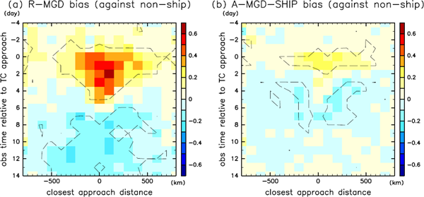
In Section 5, we demonstrated that the additional OI of the in-situ observations reduces the misfit between the in-situ observation and analyzed SST product. However, the quality of the analysis is not fully guaranteed because the observed SSTs used for the assimilation possibly deviate from true SSTs. To ensure the robustness of the current approach, the observations were separated into two subsets for data assimilation and validation. That is, we conducted an additional experiment in which the OI product by assimilating only ship-based SSTs (referred to as A-MGD-SHIP) and validated against non-ship platforms, i.e., drifting buoys, moored buoys, and Argo floats. Figure 19 shows that the A-MGD-SHIP is better than the R-MGD in that the biases were almost halved even against independent observations, although we assign the large observation errors to the ship-based observations. This validation ensures the robustness of the current approach.
8. Concluding remarks
In this study, the potential biases in the near-realtime merged satellite and in-situ data Global Daily SST of the JMA (abbreviated as R-MGD) with respect to in-situ observations were quantified along the passage of TCs in the western North Pacific by focusing on the temporal filters used in the R-MGD analysis. The case study and composite analysis exhibited that positive biases occurred when the SST dropped rapidly in a few days after the passage of TCs whereas negative biases typically occurred when the SST was restoring one week after the passage. During August–September 2020, the biases reached more than +2°C. It is explained by the availability of the data as the near-real-time product and exceedingly gentle temporal changes in the R-MGD system, which filters out short-time-scale fluctuations that occurred during the “less than 27-day” period. The positive SST bias is largely associated with the cold subsurface water and intense TCs, and thus, the positive biases are notable in the East China Sea, Yellow Sea, Sea of Japan, and in the southeast of Japan and Ryukyu Islands, except around the Kuroshio and Kuroshio extension regions. In fact, storm-induced SST biases in the composite analysis might be underestimated because some actual observations were classified into non-“best-quality” categories due to the rapid changes. This issue is discussed in Supplement 3.
It is encouraging that the OI of the in-situ observations obtained within 72 h prior to the R-MGD analysis time can alleviate these biases because this process can add more information on short-term fluctuations. Because our additional OI system is very simple, it strongly suggests that the consideration of shortterm fluctuations is indispensable to diminish the SST biases. Although the proposed approach is computationally cheap and can be easily implemented upon the existing system, we do not insist that this approach is the best for improving the quality of SST analysis. An alternative approach is to assign more weights to short-term scale features from satellites or to use a sophisticated oceanic data assimilation technique such as a four-dimensional variational data assimilation system that employs the ocean model dynamics to constrain the SST field where the observations are not available. Furthermore, we can assign the previous SST analysis as a first guess and digest the satellite and in-situ observations within a few days through the OI as in OSTIA, which suffers much less TC-induced SST biases (Supplement 2). In May 2021, the JMA publicized a future plan to incorporate short-termfluctuations in the global SST analysis by replacing MGDSST with the global HIMSST (https://www.jma.go.jp/jma/kishou/shingikai/kondankai/suuchi_model_kondankai/part5/part5-shiryo1.pdf). Although the SST biases in HIMSST are slightly smaller than those in the R-MGD (Supplement 4), a careful comparison of various approaches in terms of the benefits and risks is preferable toward further improvements.
The SST biases in the R-MGD after the passage of TCs may not be favorable in weather and ocean forecasts because the biases bring about persistent errors in the JMA systems. To quantify the contribution of the updated SST on weather forecasts, we conducted 51 5-day forecasts with the R-MGD and A-MGD. The updated SST generally yields better TC intensity forecasts. However, the evaluation for predicting high-impact weather events seems to require more samples, which will be a future topic. Also, further improvements may come from the data assimilation system inheriting the updated weather fields as the first guess in the next cycle and the lateral boundary condition out of the improved global-model forecasts.
We have not evaluated the forecast skills of heavy rainfall events with a high-resolution model. It is another future topic that should be investigated in the near future. For example, heavy rainfall events in Japan are very sensitive to the SST in the East China Sea or Sea of Japan (Iizuka and Nakamura 2019; Manda et al. 2014; Moteki and Manda 2013) as well as the TC forecasts (Emanuel 1986; Ito and Ichikawa 2021; Nayak and Takemi 2019). The Northern-Kyushu heavy rainfall event in 2017, Western-Japan heavy rainfall event in 2018, and TC Haishen in 2020 occurred just after the passage of TCs Nanmadol (in 2017), Prapiroon (in 2018), and Bavi and Maysak (in 2020) in the East China Sea and Sea of Japan, respectively. The prediction skill of such events could be enhanced if the high-quality SST analyses were used. As such, the bias of near-real-time SST should be resolved not only for daily forecasts but also for disaster prevention and mitigation.
Although we have mainly focused on the TC-related SST biases of the R-MGD in the western North Pacific, the biases in the other basins and products are described in the Supplements. Supplement 1 shows that D-MGD contains negative (positive) biases at the analysis time before (after) the closest approach of a TC as expected in Figs. 2c, d. Supplement 2 shows the global analysis of TC-related SST biases in the R-MGD and OSTIA. It shows that the biases of the R-MGD were found in all basins and the biases are much smaller in OSTIA. Supplement 3 discusses the possible underestimation of SST biases in this work arising from the inappropriate QCs of the in-situ dataset. When the TC-induced SST decrease is very rapid, the in-situ SST observations can be regarded as suspicious presumably because of the large deviation from the background SST. Thus, the biases with respect to the true SST might be larger than those in the main text. In Supplement 4, the monthly mean SST errors in A-MGD are smaller than those in the R-MGD even with the observations outside of TCs. Supplement 5 shows that the time lag between the SST analysis time and initial time of JMA global-model forecasts can increase SST biases in the forecast system. In turn, the frequent update of SST can slightly decrease the SST biases. Supplement 6 describes the TC-related SST biases in HIMSST. The biases of HIMSST are slightly smaller compared to those of the R-MGD. The assimilation of in-situ observations recorded within 72 h through additional OI further decreases these biases. These supplements are useful for a practical application and further developments.
Supplements
Supplement 1 shows the SST biases in D-MGD. Supplement 2 shows the global analysis of TC-related SST biases in the R-MGD and OSTIA. Supplement 3 analyzes the SST biases, including the low-quality dataset. Supplement 4 describes the SST errors, including the observations outside of TCs. Supplement 5 shows the dependence of SST biases on the reference time. Supplement 6 describes the TC-related SST biases in HIMSST.
Acknowledgments
We thank Dr. Naoki Hirose, Dr. Masahiro Sawada, Dr. Soichiro Hirano, Dr. Udai Shimada, Dr. Yosuke Fujii, Dr. Takahiro Toyoda, Dr. Kei Sakamoto, Ms. Mieko Seki, and the JMA Office of Marine Prediction for valuable information and comments. This work was supported by the University of the Ryukyus Research Project Promotion Grant (Strategic Research Grant 18SP01302) and MEXT KAKENHI (Grant JP18H01283). SSTs at the KEO buoy were provided by the OCS Project Office of NOAA/PMEL. AMSR2 data used in this paper was supplied by the GHRSST Server, Japan Aerospace Exploration Agency. This work is done for the author's research purposes and should not be regarded as official JMA views.
Footnotes
1 Using a Fourier transform, the ratio r between the input and output power spectra is r = exp[−2π2 (σ2x/λ2x + σ2y/λ2y + σ2t/T2)]. Thus, the output power spectrum was half of the input, r = 1/2, in the time scale of T = 27.0 days for σt ≈ 5.06 days and T = 53.0 days for σt ≈ 9.93 days if the dataset was sufficiently long in time. In fact, the output power spectrum is more than half for 27 days and 53 days because the data length is not sufficient. Although the terms “27-day filter” and “53-day filter” are inappropriate in this sense, we use these terms following the convention. The same notion is applied to spatial filtering.
2 We cannot evaluate the influence of observation depths because they are not recorded for shipship-based observations in iQuam.
References
- Dare, R. A., and J. L. McBride, 2011: Sea surface temperature response to tropical cyclones. Mon. Wea. Rev., 139, 3798-3808.
- Donlon, C. J., M. Martin, J. Stark, J. Roberts-Jones, E. Fiedler, and W. Wimmer, 2012: The Operational Sea surface temperature and Sea Ice Analysis (OSTIA) system. Remote Sens. Environ., 116, 140-158.
- Emanuel, K. A., 1986: An air-sea interaction theory for tropical cyclones. Part I: Steady-state maintenance. J. Atmos. Sci., 43, 585-605.
- Hirose, N., N. Usui, K. Sakamoto, H. Tsujino, G. Yamanaka, H. Nakano, S. Urakawa, T. Toyoda, Y. Fujii, and N. Kohno, 2019: Development of a new operational system for monitoring and forecasting coastal and open-ocean states around Japan. Ocean Dyn., 69, 1333-1357.
- Huang, B., W. Wang, C. Liu, V. Banzon, H.-M. Zhang, and J. Lawrimore, 2015: Bias adjustment of AVHRR SST and its impacts on two SST analyses. J. Atmos. Oceanic Technol., 32, 372-387.
- Iizuka, S., and H. Nakamura, 2019: Sensitivity of midlatitude heavy precipitation to SST: A case study in the Sea of Japan area on 9 August 2013. J. Geophys. Res.: Atmos., 124, 4365-4381.
- Ikawa, M., and K. Saito, 1991: Description of a nonhydrostatic model developed at the Forecast Research Department of the MRI. Technical Reports of the Meteorological Research Institute, 28, Japan Meteorological Agency, 238 pp.
- Ishii, M., A. Shouji, S. Sugimoto, and T. Matsumoto, 2005: Objective analyses of sea-surface temperature and marine meteorological variables for the 20th century using ICOADS and the Kobe Collection. Int. J. Climatol., 25, 865-879.
- Ito, K., and H. Ichikawa, 2021: Warm ocean accelerating tropical cyclone Hagibis (2019) through interaction with a mid-latitude westerly jet. SOLA, 17A, 1-6.
- Ito, K., T. Kuroda, K. Saito, and A. Wada, 2015: Forecasting a large number of tropical cyclone intensities around Japan using a high-resolution atmosphere-ocean coupled model. Wea. Forecasting, 30, 793-808.
- Japan Meteorological Agency, 2017: Climate change monitoring report 2016. Japan Meteorological Agency, 100 pp. [Available at https://www.jma.go.jp/jma/en/NMHS/ccmr/ccmr2016_high.pdf.]
- Japan Meteorological Agency, 2019: Outline of the operational numerical weather prediction at the Japan Meteorological Agency (March 2019). Japan Meteorological Agency, 242 pp. [Available at https://www.jma.go.jp/jma/jma-eng/jma-center/nwp/outline2019-nwp/index.htm.]
- Japan Meteorological Agency, 2021: Annual Report of Numerical Prediction Development Center 2020. JMA Numerical Prediction Development Center, 158 pp (in Japanese). [Available at https://www.jma.go.jp/jma/kishou/books/npdc/npdc_annual_report_r02.pdf.]
- Kain, J. S., and J. M. Fritsch, 1990: A one-dimensional entraining/detraining plume model and its application in convective parameterization. J. Atmos. Sci., 47, 2784-2802.
- Kanada, S., H. Aiki, K. Tsuboki, and I. Takayabu, 2021: Future changes of a slow-moving intense Typhoon with global warming: A case study using a regional 1-km-mesh atmosphere–ocean coupled model. SOLA, 17A, 14-20.
- Kitagawa, H., 2000: Radiation processes. Separate volume of annual report of JMA-NPD, 46, 16-31. Japan Meteorological Agency (in Japanese).
- Kobayashi, S., Y. Ota, Y. Harada, A. Ebita, M. Moriya, H. Onoda, K. Onogi, H. Kamahori, C. Kobayashi, H. Endo, K. Miyaoka, and K. Takahashi, 2015: The JRA-55 Reanalysis: General specifications and basic characteristics. J. Meteor. Soc. Japan, 93, 5-48.
- Kurihara, Y., T. Sakurai, and T. Kuragano, 2006: Global daily sea surface temperature analysis using data from satellite microwave radiometer, satellite infrared radiometer and in-situ observations. Wea. Bull., 73, S1-S18 (in Japanese).
- Kusunoki, S., and R. Mizuta, 2008: Future changes in the Baiu rain band projected by a 20-km mesh global atmospheric model: Sea surface temperature dependence. SOLA, 4, 85-88.
- Lin, I.-I., C.-C. Wu, I.-F. Pun, and D.-S. Ko, 2008: Upper-ocean thermal structure and the western North Pacific category 5 typhoons. Part I: Ocean features and the category 5 typhoons' intensification. Mon. Wea. Rev., 136, 3288-3306.
- Lin, S., W.-Z. Zhang, S.-P. Shang, and H.-S. Hong, 2017: Ocean response to typhoons in the western North Pacific: Composite results from Argo data. Deep Sea Res. Part I: Oceanogr. Res. Pap., 123, 62-74.
- Manda, A., H. Nakamura, N. Asano, S. Iizuka, T. Miyama, Q. Moteki, M. K. Yoshioka, K. Nishii, and T. Miyasaka, 2014: Impacts of a warming marginal sea on torrential rainfall organized under the Asian summer monsoon. Sci. Rep., 4, 5741, doi:10.1038/srep05741.
- Mei, W., and C. Pasquero, 2012: Restratification of the upper ocean after the passage of a tropical cyclone: A numerical study. J. Phys. Oceanogr., 42, 1377-1401.
- Moteki, Q., and A. Manda, 2013: Seasonal migration of the Baiu frontal zone over the East China Sea: Sea surface temperature effect. SOLA, 9, 19-22.
- Nakanishi, M., and H. Niino, 2004: An improved Mellor–Yamada Level-3 model with condensation physics: Its design and verification. Bound.-Layer Meteor., 112, 1-31.
- Nayak, S., and T. Takemi, 2019: Quantitative estimations of hazards resulting from Typhoon Chanthu (2016) for assessing the impact in current and future climate. Hydrol. Res. Lett., 13, 20-27.
- Price, J. F., 1981: Upper ocean response to a hurricane. J. Phys. Oceanogr., 11, 153-175.
- Price, J. F., R. A. Weller, and R. Pinkel, 1986: Diurnal cycling: Observations and models of the upper ocean response to diurnal heating, cooling, and wind mixing. J. Geophys. Res., 91, 8411-8427.
- Price, J. F., T. B. Sanford, and G. Z. Forristall, 1994: Forced stage response to a moving hurricane. J. Phys. Oceanogr., 24, 233-260.
- Price, J. F., J. Morzel, and P. P. Niiler, 2008: Warming of SST in the cool wake of a moving hurricane. J. Geophys. Res., 113, C07010, doi:10.1029/2007JC004393.
- Reynolds, R. W., and T. M. Smith, 1994: Improved global sea surface temperature analyses using optimum interpolation. J. Climate, 7, 929-948.
- Reynolds, R. W., N. A. Rayner, T. M. Smith, D. C. Stokes, and W. Wang, 2002: An improved in situ and satellite SST analysis for climate. J. Climate, 15, 1609-1625.
- Saito, K., 2012: The JMA nonhydrostatic model and its applications to operation and research. Atmospheric Model Applications. Intech, 85-110.
- Saito, K., T. Fujita, Y. Yamada, J. Ishida, Y. Kumagai, K. Aranami, S. Ohmori, R. Nagasawa, S. Kumagai, C. Muroi, T. Kato, H. Eito, and Y. Yamazaki, 2006: The operational JMA nonhydrostatic mesoscale model. Mon. Wea. Rev., 134, 1266-1298.
- Sakai, R., and M. Yamaguchi, 2005: The WGNE intercomparison of tropical cyclone track forecasts by operational global models. CAS/JSC WGNE Res. Activ. Atmos. Oceanic Modell., 35, 0207-0208.
- Sakamoto, K., H. Tsujino, H. Nakano, S. Urakawa, T. Toyoda, N. Hirose, N. Usui, and G. Yamanaka, 2019: Development of a 2-km resolution ocean model covering the coastal seas around Japan for operational application. Ocean Dyn., 69, 1181-1202.
- Shay, L. K., 2010: Air-sea interactions in tropical cyclones. Global Perspectives on Tropical Cyclones: From Science to Mitigation. Chan, J. C. L., and J. D. Kepert (eds.), World Scientific, 4, 93-131.
- Tsuguti, H., and T. Kato, 2014: Contributing factors of the heavy rainfall event at Amami-Oshima Island, Japan, on 20 October 2010. J. Meteor. Soc. Japan, 92, 163-183.
- Tsujino, H., H. Nakano, K. Sakamoto, S. Urakawa, M. Hirabara, H. Ishizaki, and G. Yamanaka, 2017: Reference Manual for the Meteorological Research Institute Community Ocean Model version 4 (MRI.COMv4). Technical Reports of the Meteorological Research Institute, 80, Japan Meteorological Agency, 306 pp.
- Usui, N., S. Ishizaki, Y. Fujii, H. Tsujino, T. Yasuda, and M. Kamachi, 2006: Meteorological Research Institute multivariate ocean variational estimation (MOVE) system: Some early results. Adv. Space Res., 37, 806-822.
- Usui, N., T. Wakamatsu, Y. Tanaka, N. Hirose, Takahiro Toyoda, S. Nishikawa, Y. Fujii, Y. Takatsuki, H. Igarashi, H. Nishikawa, Y. Ishikawa, T Kuragano, and M. Kamachi, 2017: Four-dimensional variational ocean reanalysis: A 30-year high-resolution dataset in the western North Pacific (FORA-WNP30). J. Oceanogr., 73, 205-233.
- Wu, Q., and D. Chen, 2012: Typhoon-induced variability of the oceanic surface mixed layer observed by Argo floats in the western North Pacific Ocean. Atmos.-Ocean, 50, 4-14.
- Xu, F., and A. Ignatov, 2014: In situ SST quality monitor (iQuam). J. Atmos. Oceanic Technol., 31, 164-180.
- Yablonsky, R. M., and I. Ginis, 2009: Limitation of onedimensional ocean models for coupled hurricane–ocean model forecasts. Mon. Wea. Rev., 137, 4410-4419.
- Yabu, S., S. Murai, and H. Kitagawa, 2005: Clear sky radiation scheme. Separate volume of annual report of JMA-NPD, 51, 53-64 (in Japanese).
- Zhang, H.-M., R. W. Reynolds, and T. M. Smith, 2004: Bias characteristics in the AVHRR sea surface temperature. Geophys. Res. Lett., 31, L01307, doi:10.1029/2003GL018804.