メソスケールの流れを解像したシミュレーションを基にした下層雲のエネルギー平衡モデルの構築

Abstract

This study proposes a new energy balance model to determine the cloud fraction of low-level clouds. It is assumed that the horizontal cloud field consists of several individual cloud cells with a similar structure. Using a high–resolution simulation dataset with a wide numerical domain, we conducted an energy budget analysis. Here we show that the energy injected into the domain by surface flux is approximately balanced with that loss due to radiation and advection due to large–scale motion. The analysis of cloud cells within the simulated cloud field showed that the cloud field consists of a number of cloud cells with similar structures. We developed a simple model for the cloud fraction from the energy conservation equation. The cloud fraction determined using the model developed in this study was able to quantitatively captured the simulated cloud fraction.

1. Introduction

Low-level clouds, such as stratocumulus or shallow cumulus, play an important role in determining the radiation budget of the globe because such clouds cover a wide area and reflect shortwave radiation (Klein and Hartmann 1993; Klein et al. 1995; Wood 2012; Zelinka et al. 2016). These clouds exist at low altitudes (z < 2 km) with a depth of several hundred meters. Satellite observations have revealed that the horizontal fields of these low–level clouds have cellular structures and that there are several kinds of horizontal cloud patterns (Krueger and Fritz 1961; Stevens et al. 2005b; Wood and Hartmann 2006; Comstock et al. 2007). Two major patterns are open cell and closed cell structures (Koren and Feingold 2013). The former pattern accompanies a cumulus–like flow and cloud structures, i.e., narrow updraft and wide downdraft regions. Horizontally, the low-level cloud field covers hundreds of square kilometers and consists of a number of cloudy cells in which each cell has a circulation with a horizontal scale of several kilometers. The large areas of the planet covered by these low–level clouds have a significant influence on the global radiation budget.

Various physical processes that cover a wide range of spatiotemporal scales are important for the development and maintenance of low-level clouds, and these range from interaction between aerosol and cloud droplets to large-scale motion (e.g., the subsidence branch of the Hadley circulation). (Bretherton and Wyant 1997; Wyant et al. 1997; Bretherton et al. 1999) For instance, when the number of cloud condensation nuclei (CCN) is small, large water droplets form in a saturated environment, and these are more likely to fall as rain. This precipitation (drizzle) greatly changes the cloud structure and causes a structural transition from closed cell to open cell (Xue et al. 2008; Caldwell and Bretherton 2008; Stevens and Feingold 2009; Wang and Feingold 2009a, b; Feingold et al. 2010, 2015; Berner et al. 2011; Yamaguchi and Feingold 2015). Another example representing the importance of various scales for low–level clouds is buoyancy reversal near a cloud top, in which entrainment of dry air aloft into the cloud layer promotes evaporation and cooling, and downward motion is accelerated, resulting in a reducing stratocumulus cloud deck (Yamaguchi and Randall 2008; Mellado 2010; Mellado et al. 2010, 2014; Noda et al. 2013, 2014; van der Dussen et al. 2014).

Because of the importance of small-scale microphysical processes, it is difficult to explicitly resolve the low–level clouds in global atmospheric models. Even a global simulation with a grid spacing of 870 m (Miyamoto et al. 2013; Kajikawa et al. 2016; Yashiro et al. 2016) has difficulty to accurately simulate the low–level clouds and hence cloud fraction. A number of studies have investigated low-level clouds using the grids with a resolution of O(10) m (Moeng et al. 1996; Stevens et al. 2005a; Ackerman et al. 2009; Yamaguchi and Feingold 2012; Sato et al. 2015a, b). These studies successfully simulated the low–level clouds, i.e., the resolved scale needs to be in the order of 10 m (unresolved scale is less than this scale) to realistically simulate the low–level clouds. In other words, one of the dominant mechanisms governing these clouds is of this order. As the global radiation budget is affected by low–level clouds, global models, especially for long-term simulations such as climate simulations, need to properly incorporate their effects, and hence a deeper understanding of these low–level clouds would be beneficial.

Previous studies have studied energy and water budget in the atmospheric boundary layer by assuming an equilibrium state (Lilly 1968; Schubert 1976; Albrecht et al. 1979; Betts 1976; Betts and Ridgway 1989; Neggers et al. 2006). Caldwell et al. (2005) conducted budget analyses for mass, heat and liquid water static energy in the boundary layer by observation and reanalysis data to examine the entrainment at the top of boundary layer. Kalmus et al. (2014) also conducted budget analyses based on a set of satellite, GPS, and ship-based data. They found that in climatological mean, the transition from stratocumulus to cumulus state is associated with an increase in surface latent heat flux, boundary layer height, rain, and horizontal advection of dry air and a decrease in entrainment of dry air. Chung et al. (2012) showed from an energy budget analysis based on a series of large–eddy simulations (LESs) that the temperature tendency due to radiative cooling is balanced with the tendency due to the subsidence warming during the transition of cloud regime. They derived an equation for cloud fraction based on the balance of two tendency terms. However, the numerical domain of their simulation covered horizontally 3.2 × 3.2 km², which is not large enough an area to resolve mesoscale motions.

A notable feature of low–level clouds is that the cloud field consists of a number of cloudy cells, each of which has similar flow and cloud structures. The open- and closed cell flow fields are similar to the Rayleigh–Bénard convection (Krishnamurti 1975; Laufersweiler and Shirer 1989; Weidauer et al. 2010, 2011; Miyamoto et al. 2020). The convection transports heat vertically via a number of cloud cells that have a flow structure similar to each other. In fact, many of the previous studies on low clouds introduced above implicitly state that the cloud field consists of similar cloud cells. This unique feature of low-level clouds is one of the key assumptions on which the present study is based.

In this study, we develop an energy balance model for low-level clouds, based on the key assumption that the cloud field consists of a number of cloud cells with the same structure, and we use the model to conduct an energy budget analysis of a simulated cloud field. We use the high-resolution simulation with a wide numerical domain conducted by Sato et al. (2015b) for our analysis. The simulation setting and methodology used to analyze the cloud cells are described in Section 2. An overview of the simulation of Sato et al. (2015b) and the results of the detected cloud cells are presented in Section 3. An energy budget analysis is performed and an energy balance model is presented in Section 4. The results are discussed in Section 5 and we present our conclusions in Section 6.

2. Experimental setup and extraction of cloud cells

2.1 Simulation design of Sato et al. (2015b)

We analyzed the results of the idealized numerical simulation in Sato et al. (2015b), which covers (768, 28, 2) km in the (x*, y, z) directions with grid intervals of (50, 50, 5) m. A fully compressible numerical model, Scalable Computing for Advanced Library and Environment (SCALE) (Nishizawa et al. 2015; Sato et al. 2015a), was used for the integration. The prognostic quantities generated by SCALE were the density of the total mass, three-dimensional momentum, potential temperature weighted by density, and microphysical quantities (mixing ratio of water vapor, and mass and number density of cloud water, rain water, ice, snow, and graupel). The time differential was discretized using the three-step Runge–Kutta scheme. The advection and pressure gradient terms were discretized using the fourth- and second-order accuracies, respectively. The discretized equations were solved explicitly for both the horizontal and vertical directions.

The number of grid squares was 6144 × 564 × 275. The grid spacing was vertically stretched above 1.2 km, and also horizontally in 0 km < x* < 247 km, and 545 km < x* < 768 km. From x* = 247 km to 545 km, the grids were evenly allocated every 50 m, which is the analysis domain and hereafter we focus on this region. x* = 245 km is defined as the upwind boundary (x = 0). The boundary conditions for the x* and y directions were open and periodic, respectively. The effects of sub-grid-scale turbulence were solved using a Smagorinsky scheme generalized for anisotropic grids (Smagorinsky 1963; Lilly 1962; Scotti et al. 1993). Cloud physical processes were calculated using double moment-bulk cloud microphysics (Seifert and Beheng 2006; Seiki and Nakajima 2014). The nucleation was represented by assuming a temporally constant number of CCN. Longwave radiation was only considered in the simulation and vertical radiation fluxes were solved following Stevens et al. (2005a). The inversion height used in the radiation scheme was defined as the level at which the total water mixing ratio q_t became less than 8.0 g kg⁻¹. In the horizontally stretched regions and the topmost 500-m depth of the domain, Rayleigh damping was applied to all of the prognostic variables to prevent artificial reflection of gravity waves. The timescales used for the damping were 300 s and 10 s for the horizontal and vertical directions, respectively.

The initial vertical profiles for the temperature T and water vapor mixing ratio q_v were constructed from an observation campaign, Second DYnamics and Chemistry Of Marine Stratocumulus (DYCOMS-II) RF02 (Ackerman et al. 2009). The effect by largescale subsidence (w_LS = D_z) was given to all prognostic variables (Ackerman et al. 2009), where D was 1.33 × 10⁻⁶ s⁻¹, the same as that used in Berner et al. (2011). The integration period was 16 hours. The numerical simulation was initialized from horizontally uniform fields for all quantities except the surface heat fluxes and number of CCN, which were changed in the streamwise (x*) direction. Surface fluxes for sensible and latent heat were 15 W m⁻² and 93 W m⁻² at x* = 247 km, and the fluxes increased at a rate of 0.03062 W m⁻² km⁻¹ and 0.1365 W m⁻² km⁻¹ in the x* direction, respectively. Thus, the sensible and latent heat fluxes were 24.12476 W m⁻² and 133.677 W m⁻² at the downwind edge. The equations for surface fluxes for sensible and latent heat were given by   

  

and hence the surface enthalpy flux was given by   

CCN decreased according to 250 exp(−7.0433x* × 10⁻⁶) cm⁻³ and CCN at the downwind edges was 5.38094 cm⁻³. Both the surface fluxes and CCN were fixed during the simulation. A uniform velocity of 5 m s⁻¹ was present in the x* direction in the initial field. The parameterization of Stevens et al. (2005a) was used for the net radiative longwave flux.

  

Here, and are the integrated liquid water mixing ratio in the vertical direction, F_R0 = 70 W m⁻², F_R1 = 22 W m−2, ρ_zi is the air density at the cloud top level z_i, D_s = 3.75 × 10⁻⁶ s⁻¹, and a_z = 1 m^−4/3. More specific information on the experimental setting can be found in (Sato et al. 2015b).

The analysis domain (245 km < x* < 545 km; i.e., excluding the buffer regions) was divided into 10 subdomains for the subsequent analysis. Each subdomain covers (30, 28, 2) km in the (x, y, z) directions and is referred to as R00, R01, …, and R09.

2.2 Detection algorithm of for cloud cells

We developed a method that is able to detect cloud cells in a simulated cloud field based on an approach designed for deep convection (Miyamoto et al. 2013, 2015, 2016). First, vertical velocity was vertically averaged in the boundary layer, and horizontally smoothed 100 times by applying a 1-2-1 filter. Second, the grid point of the cell center was defined as a grid point having a local peak of vertical velocity relative to the standard deviation of vertical velocity obtained in a subdomain, σ_w. Specifically, grid points, at which the absolute vertical velocity exceeded the standard deviation; i.e., |w| > σ_w, were detected as the cell center. We used the standard deviation to search for strongly (anomalously) deviated peaks in the subdomains. Since the methodology applies the absolute velocity, the method can capture positive and negative peaks in vertical velocity. In the simulation, positive peaks were detected. Once a center grid was detected, the coordinates were transformed into cylindrical coordinates around the detected cell center.

3. Results

3.1 Overview of Sato et al. (2015)

Figure 1 shows the horizontal distribution of the liquid water path (LWP) at seven selected simulation times. The cloud field shows cellular structures at all times. The spatial scale, or distance between cellular structures, increases with time, especially on the downwind side (right hand side of panels). At the same time the spatial scale of the cloud cell itself becomes also larger. The horizontal cloud field on the upwind side looks like the cloud structure of a closed cell (Wood 2012), whereas that on the downwind side appears to be an open cellular structure. Nevertheless, the analysis undertaken by Sato et al. (2015b) indicates that the cell structure on the upwind side is an open cell. Horizontal cross sections of vertical velocity at selected four regions (R01, R03, R05, and R07) at t = 16 h are depicted in Fig. 2. The cellular structure is observed as seen in the LWP and the spatial scale of the cell is large in the downwind region. In particular, there are a number of vertical velocity peaks in R01. The vertical velocity is positively large at the edge of the cellular structure, especially in R03–R07.

Fig. 1.

Horizontal cross sections of liquid water path (LWP, g m⁻²) at 7 selected timesteps. The abscissa and ordinate represent the streamwise and spanwise directions, respectively, and the units are kilometers.

Fig. 2.

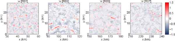
Horizontal sections of vertical velocity at an altitude of 400 m at t = 16 h for R01, R03, R05, and R07. The units of the color bar are m s⁻¹. The abscissa indicates the distance from x = 0.

Figure 3 shows a time series of the cloud fraction, which is defined as the fractional area where LWP is greater than 80 g m⁻² in each subdomain. The cloud fraction is close to 1.0 in all subdomains at the beginning of the simulation, which indicates that the entire domain is covered by clouds immediately after the simulation begins. The temporal changes in cloud fraction are similar in all subdomains, whereas the magnitudes differ; i.e., the magnitude decreases after integration begins and then remains at a constant value after t = 12 h. On the upwind side (R01 or R02), the magnitude remains large throughout the simulation. In contrast, the cloud fraction rapidly decreases to 0.7 on the downwind side (R06–R09).

Fig. 3.

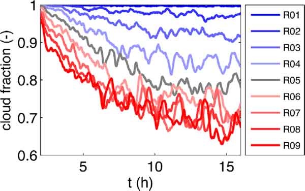
Time series of the cloud fraction (dimensionless) of the regions, which is defined as the ratio of the area with an LWP higher greater than 80 g m⁻² to that of the entire region. The numbers in the legend indicate the regions from 1 to 9.

Figure 4 shows vertical profiles of the temperature, water vapor mixing ratio, cloud water mixing ratio q_c , rain water mixing ratio q_r, and vertical fluxes of the four quantities in R01, R03, R05, and R07. The quantities are temporally averaged from t = 12 h to 16 h and horizontally averaged, whereas the fluxes are integrated in each subdomain. T decreases with height up to z = 0.85 km, then rapidly increases to 292 K, and is constant above. q_v has a peak at the surface, decreases with height, rapidly decreases at z = 0.85 km, and is nearly constant above. q_v is large, especially at lower levels, which most likely results from surface fluxes. The larger T and q_v in the downwind region are caused by the increased surface heat flux. q_c has a peak below the inversion height and it is large in the upwind region. The vertical profiles of q_r are similar in the four subdomains, showing a peak below that of q_c and a non-zero value at the surface.

Fig. 4.

Vertical profi les of (upper) temperature (K), water vapor mixing ratio (g kg⁻¹), cloud water mixing ratio (g kg⁻¹), rain water mixing ratio (g kg⁻¹), liquid-water potential temperature (K), and (lower) vertical fluxes of temperature (K m s⁻¹) and water mixing ratios (g kg⁻¹ m s⁻¹). The quantities in the upper panels are horizontally averaged and the fl uxes in the lower panels are horizontally integrated in each subdomain. They are averaged from t = 12 h to 16 h. The dashed lines in the panels, (a), (b), and (e), indicate the initial values.

Vertical profiles of the area-integrated vertical flux of the four quantities in the four subdomains are shown in Figs. 4e–h. The fluxes are the sum of the grid-scale and subgrid–scale components. The temperature flux is smaller in the downwind region (Fig. 4e) and is generally positive, except around the bottom and top of the cloud layer. It decreases from the surface to z = 0.3 km, increases with height up to about 0.7 km, and then decreases again at the inversion height. The vertical fluxes of q_v are not significantly different in the four subdomains (Fig. 4f) and monotonically decrease with height from the surface to the inversion height. The vertical flux of q_c is largest at the peak altitude of q_c , and is large in the upwind region. The vertical profi le of the fl ux of q_r has a negative peak at z = 0.28 km and a positive peak at z = 0.78 km. We note that the flux of q_r does not include the precipitation fl ux in which the water droplets fall by gravity.

3.2 Structure of cloud cells

In order to examine the cell structure in the subdomains, we developed a methodology for cell detection. The cloud cell detection method was applied to the vertical velocity field (cf. Fig. 2) from t = 12 h to 16 h. Figure 5 shows the number of detected cells for each region averaged over the analysis period in each subdomain. The number is larger on the upwind side, with the largest being 12 in R02, whereas it is 7–8 on the downwind side. The tendency of the number of cells is consistent with a visual inspection of Figs. 1 and 2.

Fig. 5.

Number of detected cloud cells averaged from t = 12 h to 16 h in each subdomain.

To evaluate the proposed method, we tested the sensitivity of the number of detected cells by changing the number of smoothing processes and the threshold for the vertical velocity. In particular, by introducing a factor, B, to the definition |w| > Bσ_w, two values, B = 0.5 and 2.0, were tested. The top panels in Fig. 6 show the number of detected cells when B = 0.5 (left) and B = 2.0 (right). Overall, the number of cells was not largely changed by the thresholds, whereas the sensitivities of the number of detected cells to the two parameters were reasonable. Compared with the control value B = 1.0 (Fig. 5), the number slightly increased and decreased when the factor B decreased and increased, respectively.

Fig. 6.

Same as Fig. 5, but for (a) B = 0.5, (b) B = 2.0, (c) number of smoothing, N = 50, and (d) number of smoothing, N = 200.

Next, the number of smoothing N was also tested by applying N = 50 and 200, of which results of detection are shown in the bottom panels in Fig. 6. The number of cells was not largely sensitive to the number of smoothing; the cell number was slightly reduced when the number of smoothing was 200, while the number did not change when the number of smoothing was reduced to 50 times.

Figure 7 shows a radius–height cross section of the radial and vertical velocities, which are composites of all of the cloud cells detected. The radial velocity has a positive peak immediately below the inversion height, and a negative peak above the surface, both of which are located at a radius of several hundred meters. The vertical velocity has a positive peak at the cell center.

Fig. 7.

Radius–height sections of (top) radial velocity and (bottom) vertical velocity for R01, R03, R05, and R07, which are composites of all samples from the cloud cells. Units: m s⁻¹. Positive radial velocity directs radially outward.

The outside is the downward region, while the magnitude of the downward velocity is much smaller than that of upward velocity. The flow fields in the vertical cross section are qualitatively the same in the subdomains. This indicates that circulation is present in the cell with the inward flow at the bottom, upward motion at the convection center, and outward motion at the top of the boundary layer. The flow field is confined to a small area on the upwind side, whereas the magnitude of the vertical velocity is almost the same among the subdomains.

Radius–height sections of q_c and q_r are shown in Fig. 8. The detected cells in all subdomains have a cloud layer approximately from z = 550 m to 850 m, a peak of w at the core, and q_r immediately outside the core. The region of high q_r extends from the upper layer to the surface in the downwind region, indicating that the precipitation reaches the ground. The precipitation is large on the downwind side. The composites of velocity and water substance have also been produced by Zhou and Bretherton (2019). The present result is qualitatively the same as the previous study, whereas the methodology to construct the composite and the simulation data are different.

Fig. 8.

Radius–height sections of the mixing ratio of (top) cloud water and (bottom) rain water for R01, R03, R05, and R07, which are composites of all samples from the cloud cells. Units: kg kg⁻¹.

Figure 9 shows radius–height cross sections of the number densities of cloud water N_c and rain water N_r. A large number density is approximately collocated with the high mixing ratio, whereas the peak of N_c is located lower than that of q_c . They have a peak at the cell center that decays radially. In particular, N_c is large in the upwind region, whereas N_r is large in the downwind region. N_c is large in the upper layer and is far outside the cell center in R01, which may be due to the presence of a neighboring cell. In contrast, N_r is large in the middle levels as well as at the peak altitude in R07.

Fig. 9.

Radius–height sections of the number density of (top) cloud water and (bottom) rain water for R01, R03, R05, and R07, which are composites of all samples from the cloud cells.

Figure 10a shows the radial profiles of the vertical difference in radiation flux between the surface and cloud-top level ΔF_R, which are averaged around the detected cell center, for the four selected regions. The flux difference increases radially up to around a radius of 0.9 km and then decreases. The magnitude of the radial decrease is more significant in downwind regions. The peak of the flux difference at a radius of 0.8 km is consistent with the radius–height cross sections of q_c and q_r, in which the column-integrated value is large at the radius.

Fig. 10.

(a) Radial profiles of vertical difference in radiation flux ΔF_R averaged in the detected cloud cells detected from t = 12 h to 16 h. The black, gray, red, and blue lines represent R01, R03, R05, and R07, respectively. (b) Levels of cloud top and bottom, which are defined as q_t > 0.05 g kg⁻¹, averaged in each subdomain.

The averaged cloud depth decreases in the down-wind side (Fig. 10b), which is consistent with the difference in radiation flux averaged in the cloud cells. As indicated by the horizontal LWP fields and radius–height sections, the cloud cells in the upwind side have thicker clouds than those in the downwind side. Since the thickness of the clouds does not largely differ among the subdomains (cf. Fig. 4), the flux difference mainly results from the liquid water content. This results in the variation of the vertical radiation flux in the streamwise direction as shown later.

The composite analysis shows that the structures of the cloud cells are qualitatively the same across the entire simulation domain, whereas the horizontal cloud field (Fig. 1) suggests that the cell structure changes from closed to open in the domain. This is consistent with Sato et al. (2015b), and the simulated cloud field has an open cell-like structure across the entire domain. We interpret that the horizontal cloud field is the result of cloud cells for which the distance between cells is increasing in the streamwise direction (Ovchinnikov et al. 2013; Sato et al. 2015a).

Satellite observations and numerical simulations in previous studies have suggested that the horizontal cloud field of low-level clouds consists of a number of cloud cells with the same structure (Wood and Hartmann 2006; Comstock et al. 2007). Figure 11 shows radius–height cross sections of the standard deviation of q_c and q_r. The quantities are an order of magnitude smaller than the ensemble mean (cf. Fig. 8). This is the same for other quantities, such as number densities (figure not shown). In conclusion, the simulated cloud field consists of a number of cloud cells with almost the same structure.

Fig. 11.

Radius–height sections of standard deviation of the mixing ratio of (top) cloud water and (bottom) rain water for R01, R03, R05, and R07, which are obtained from all samples from the cloud cells. Units: kg kg⁻¹.

To compare the area-integrated vertical fluxes (cf. Fig. 4) with those in the cloud cells, vertical profiles of the quantities in the cloud cells are shown in Fig. 12. The quantities were averaged (Figs. 4a–d) and integrated (Figs. 4e–h) within the 5-km radius from the center of the detected cloud cell. The vertical profiles are qualitatively the same as those averaged in the subdomains, and the order of magnitudes are also the same. Thus, the orders of total vertical fluxes for the quantities are equal to the total fluxes in the cloudy region around the detected cloud cells, whereas the profiles fluctuated. Furthermore, the differences among the four subdomains are qualitatively the same as those of the area-integrated values (Figs. 4e–h). In other words, the vertical fluxes averaged over the subdomain can be represented by the fluxes averaged in the cloud cells.

Fig. 12.

Vertical profiles of (upper) temperature (K), water vapor mixing ratio (g kg⁻¹), cloud water mixing ratio (g kg⁻¹), rain water mixing ratio (g kg⁻¹), liquid-water potential temperature (K), and (lower) vertical fluxes of temperature (K m s⁻¹) and water mixing ratios (g kg⁻¹ m s⁻¹). The quantities in the upper panels are averaged and the fluxes are integrated within the 5-km radius from the center of the detected cloud cells. They are averaged from t = 12 h to 16 h. The dashed lines in the panels, (a), (b), and (e), indicate the initial values.

3.3 Energy budget analysis

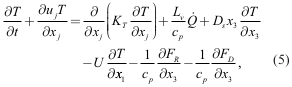
We performed an energy budget analysis for each subdomain. The conservation equation for moist enthalpy was first derived from the temperature equation and the conservation equation for water vapor by assuming incompressibility, as follows:   

  

where t is time, x_j (j = 1, 2, 3) = (x, y, z) are the spatial dimensions in a Cartesian coordinate system, u_j (j = 1, 2, 3) = (u, v, w) is velocity in the three directions, T (x, y, z, t) is temperature, q_v (x, y, z, t) is the water vapor mixing ratio, c_p is the specific heat at a constant pressure for dry air, L_v is the latent heat, K_T (x, y, z, t) is the thermal diffusion coefficient, K_q (x, y, z, t) is the diffusion coefficient for the water content, Q̇ (x, y, z, t) is the tendency of the water vapor associated with the phase change, D_s (z) is the divergence due to large-scale subsidence (s⁻¹), U is the background flow speed (m s⁻¹) and is constant across the entire domain, F_R (x, y, z, t) is the vertical radiative flux of long wave radiation, and F_D (x, y, z, t) is the vertical flux of dissipative heating. The tensor notation follows Einstein's summation convention. The left-hand-side (LHS) represents the local tendency and advection terms, and the terms on the right hand side (RHS) indicate diffusion, diabatic heating associated with phase change, large-scale divergence, advection due to the large-scale constant flow, radiative flux divergence, and frictional dissipation flux divergence, respectively. Later on, the dissipative heating term is neglected in this study, because it is not included in the present simulation.

By assuming K_T = K_q and combining the equations after c_p × (5) and L_v × (6), we obtain the conservation equation for moist enthalpy (k = c_p T + L_vq_v) as   

The equation was integrated over a volume of subdomain from the surface to the cloud top height as   

where V and A are the volume and horizontal area of the subdomain, respectively, F_sk is the surface flux of moist enthalpy into the atmosphere, Ƭ_LS (≡ D_sx₃ ∂_x3 k) represents the large-scale subsidence term, and Ƭ_CF (≡ −U∂_x1 k) represents the horizontal advection by constant flow. The first and second terms on the RHS are derived from the diffusion term and large scale divergence term in (7). We assumed that advection terms by local velocity (second term on the LHS of (7)) vanish in the integration due to the periodicity at the lateral boundaries of the subdomain, and we assumed that the enthalpy flux at the surface was F_sk and vanishes at the cloud top. The integrated equation (8) indicates that the tendency of the enthalpy in a subdomain is determined by the imbalance among the surface flux, large-scale subsidence, constant flow advection, and radiation.

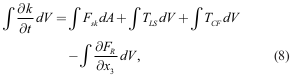Figure 13 shows the budgets of (8) calculated from the simulation averaged from t = 12 h to 16 h. The surface enthalpy flux is the dominant term that contributes positively to the system. The other terms play a negative role, and their sum corresponds approximately to the surface enthalpy flux. The radiation flux outside the cell region is nearly constant in the x direction, while the magnitude of the radiation flux in the cloud cells increases. The magnitude of large-scale subsidence is not large, but it is not negligible either, and increases toward the downwind side. The magnitude of the advection associated with the constant background velocity is the largest among the negative terms, and this is caused by a combination of the background flow (∼ 5 m s⁻¹) and the spatial enthalpy gradient. The surface flux that is large in the downwind region increases enthalpy in the air and enhances the spatial gradient of enthalpy and the horizontal advection term, while it does not largely change in the x direction.

Fig. 13.

Budget terms of the thermodynamic energy equation as a function of region (x direction), which are averaged from t = 12 h to 16 h. The fluxes are the surface flux (black solid), flux differences with minus sign due to longwave radiation in cloud cells (blue) and outside the cell region (blue dashed), divergence due to largescale subsidence (gray), horizontal advection by background wind (red), and the residual (black dashed).

4. Development of a cloud fraction model

Now we assume that the cloud field in a subdomain consists of a finite number of cloud cells with the same structure, and also that the radiation flux in the energy equation is considered separately in the cloud-cell region and other areas. By assuming that the cloud cell has a radius of r_c, (8) can be written as   

where A is the area of the subdomain, A_c is the total area of cloud cells defined by , N is the number of cloud cells in a subdomain, the tilde denotes the average inside of the cloud cell, the hat denotes the average outside of the cloud cell, and Δ is the vertical difference between the surface and the cloud top level. This equation can be written as   

where H is the depth of the cloud layer and the angle bracket indicates the domain average. We have assumed a quasi-steady state (⟨∂_tk⟩ → 0). This results in an equation for the cloud fraction as follows:   

Thus, the cloud fraction is determined from a balance between the surface enthalpy flux with large-scale subsidence and constant flow advection, and radiation fluxes in cloud cells and other areas. As the vertical difference in the radiation flux represents a flux divergence that tends to remove energy from the domain, they are negative and the minus sign on the RHS of (11) is reasonable unless the negative contribution of large-scale subsidence and the advection terms are greater than the energy input from the surface enthalpy flux. This would happen only rarely because the surface flux is on the order of 100 W m⁻², whereas the large-scale subsidence and advection terms are less than 100 W m⁻², or rather, an order of magnitude smaller than the surface flux in the focusing regions (cf. Fig. 13). The model implies that the cloud fraction increases with a large surface flux, large radiation flux, and (negatively) small effects of background flow motion. This suggests that low-level clouds cannot be present (because the cloud fraction would become less than 0) if the large-scale forcing is stronger than the surface flux; i.e., when the energy removal by largescale forcing exceeds the energy input to the system from the ocean.

Figure 14 shows the cloud fractions (temporally averaged from t = 12 h to 16 h) that were estimated from our simulation and diagnosed using (11) for each subdomain. The simulated cloud fraction monotonically decreases in the streamwise direction from 0.99 in R01 to 0.66 in R09 as shown in Figs. 1 and 3.

Fig. 14.

Cloud fraction estimated from the simulation (cf. Fig. 3) (black line) and diagnosed using Eq. (11) (gray line). The data are temporally averaged from t = 12 h to 16 h. The gray hatched area stands for the ± 1 standard deviation from the mean, which are estimated using quantities spatially averaged in each subdomain from t = 12 h to 16 h.

The diagnosed cloud fraction decreases in the streamwise direction, whereas it slightly overestimates the simulated fraction especially in the downwind regions. The standard deviation of CF, which is obtained in each subdomain from t = 12 h to 16 h, is large in the upwind regions. It is implied that the standard deviation of radiation fluxes are small in the upwind regions as the cloud field appears not to largely change in time (cf. Fig. 3). Since the radiation fluxes are in the denominator of (11) and there is no temporal variation in the surface flux in the simulation, which has the largest values among the terms in (11), it is suggested that the standard deviation of CF diagnosed by (11) is large in the upwind regions.

The relative contribution of the terms of (11) is listed in Table 1. On average, the surface flux term is the source of energy and the other terms remove the energy from the volume (cf. Fig. 13). In order to examine the sensitivity of the cloud fraction to individual terms in (11), we calculated the cloud fraction by artificially increasing the magnitude of each term by 10 % from the spatiotemporal average that was used to calculate the mean value in Fig. 14, while the others were fixed. Figure 15 shows the diagnosed cloud fraction by (11) with the magnitude of each term increased individually by 10 %. The cloud fraction is most sensitive to the surface flux, which is followed by the horizontal advection term by constant flow and the longwave radiation term in cloud cells. Although the magnitudes of change are large, it should be noted that the sensitivity has been tested by artificially increasing a single term by 10 %, while the other terms are fixed. This never happens in nature because a change in one term more or less affects other terms.

Fig. 15.

Cloud fractions estimated by Eq. (11) using the simulation, but with each term increased by 10 %. CTL is the mean shown in Fig. 14. F_s indicates the cloud fraction estimated by surface flux increased by 10 %. Similarly, HƬ_LS, HƬ_CF, −ΔF_Rc, and −ΔF_Ra indicate the cloud fraction estimated by increased vertical advection, horizontal advection, longwave radiation in cloud cells, and longwave radiation outside the cell region, respectively.

The results are summarized in Table 1, which lists the rate of change in the calculated cloud fraction. It indicates that a term with a larger mean value has a larger sensitivity as expected; the largest sensitivity of cloud fraction is found in the surface flux term, which has the largest mean value in (11). The large contribution of horizontal advection by constant flow implies the importance of representation of the wind direction as well as the wind speed in global models, while the variance of wind direction is large in models (Noda and Satoh 2014) in the Coupled Model Intercomparison Project (CMIP) (Taylor et al. 2012).

Another balance equation can be obtained by using moist conservative variables such as the liquid water potential temperature θ_l, and the concept of the present study can be applied. In this study, we consider the moist enthalpy, as it is easily obtained from T and q_c, which are the prognostic variables in the numerical model used for the present simulation.

5. Discussion

One of the applications of the model developed here to diagnose the fraction of low-level clouds is to use it as a parameterization when estimating the radiation budget of global models. The model is valid when a sufficient number of cloud cells is included in a domain that corresponds to a grid point in the global model. Specifically, the present model was developed for an area of 30 × 28 km², which is smaller than the grid spacing of conventional climate models.

The diagnostic equation has been simplified using some assumptions. Using quantities predicted or diagnosed in numerical models, terms in the numerator on the RHS of (11) (i.e., surface enthalpy flux, large-scale subsidence, and large-scale constant flow) can be calculated. Nevertheless, radiation fluxes in the cloud cell and other areas in the denominator are not explicitly estimated by climate simulations, as parameterizations are needed to calculate the fluxes from grid-scale quantities. Thus, some additional assumptions are necessary to estimate the fluxes. Once the differences in radiation fluxes are approximated using the gridscale quantities from the climate models, the cause of bias in the cloud fraction in the numerical models can be detected by comparing the estimated terms in (11) with the outputs of climate simulations.

A possible approach to estimating the vertical difference in radiation fluxes, especially the radiation flux in the cloud cell region, would be to use LWP. The present simulation uses a parameterization for radiation flux based on the vertically integrated q_l, suggesting that LWP could be a useful quantity. For example, Chung et al. (2012) proposed a method to evaluate the radiation flux term with the usage of the probability density function (pdf) of LWP. As they applied a gamma function for the pdf of LWP, the radiation flux is a function of the mean, the homogeneity, and the standard deviation of LWP. Their formulation could be applied to the present equation for the radiation flux and hence the cloud fraction. However, accurate estimation of LWP in the lower layer in climate models is also a difficult issue.

It should also be noted that the parameterization of the radiation flux (Stevens et al. 2005a) used in the present simulation is designed for nocturnal longwave radiation. Hence, a more realistic radiation scheme, such as one including short–wave radiation, would be required to apply the model to more realistic cases.

The budget equation (10) would possibly be more accurate, if the diffusion term or eddy vertical advection term at the top of boundary layer are considered, which have been neglected to derive (10). As introduced above, cloud top entrainment and shallow convection would also play important roles in determining structures of low–level clouds and these processes would be incorporated in the two terms. Further studies are needed to formulate the effects of processes at the cloud top as an area–integrated flux.

Additionally, considering the tendency term ⟨∂_tk⟩ or the advection term may also help to increase the accuracy of the CF equation (11), whereas they have been neglected as we assumed the steady state and periodicity in each subdomain. The CF shown in Fig. 14 was estimated by quantities that are averaged in a subdomain, not in time, and then the average and variance of CF were calculated. Hence, the assumption of a quasi–steady state would not work and it is desired in a future study to discuss the statistics of diagnosed CF by using different data sets, each of which individually with different quasi–steady state.

It is worth discussing the physical reason why the diagnosed CF by (11), which is derived from an energy balance equation, decreases in the streamwise direction. Let us consider a simple system in which each terms in (11) change linearly in the streamwise direction. In this case, (11) can be re-written as   

where α is the proportional coefficient for surface flux in the x direction, β is the proportional coefficient for all the other terms in the numerator of (11), γ is the coefficient for the terms in the denominator, and B₁ and B₂ are the values of the terms in the numerator and denominator at the upwind edge. Taking a spatial derivative in the x direction yields   

The condition to decrease CF in the x direction (∂_xC_F < 0) can be written as   

provided that γ > 0 and γx + B₂ > 0, which is implied by Fig. 13. The RHS of the inequality corresponds to CF (12), which is approximately 1 or less. Thus, when the ratio of coefficients in the LHS is roughly less than 1, the CF tends to decrease in the x direction. The result of the simulation (cf. Fig. 13) shows that α is positive and the largest contributor, β is small and negative, and γ is positive and large, which possibly results in the decreasing trend of CF. A large α tends to increase the CF as implied in (11), whereas large β and γ result in a decreasing trend of CF. In other words, gradual increase in surface flux and rapid decreases in large–scale effects and radiation fluxes are favorable for decrease in CF.

An increase in surface flux would enhance the LWP, which increases radiation flux in cloud cells per unit area . Since the water vapor is larger in the downwind side, a larger amount of latent heating appears to be released once condensation occurs. It is possible under an environment in which net income flux—surface flux together with the other large–scale effects that are in the numerator of the LHS of (14) and tend to decrease the increasing rate of surface flux—increases in the streamwise direction. Larger latent heating more likely produces a positive feedback between the heating and the vertical motion, which results in a larger amount of condensed water in the vertical direction and also in a smaller area (Bjerkness 1938). It increases in the streamwise direction and hence the increasing rate of radiation flux may exceed that of the net income flux. Thus, condition (14) can possibly be satisfied, indicating a decrease in diagnosed CF in the streamwise direction.

6. Conclusions

In this paper, we have proposed an energy balance model to diagnose the fraction of low-level clouds using a conservation equation of moist enthalpy and by assuming that the horizontal field of low-level clouds consists of a number of cloud cells with the same structure. The derived equation indicates that the cloud fraction can be represented as the ratio of the sum of the surface enthalpy flux, large-scale subsidence, and large-scale constant flow to the radiation fluxes in the cloud cells and other regions.

Energy budget analysis was performed on the results of a simulation covering a wide area and with fine spatial resolution. The surface flux played a dominant role in transferring energy into the domain, while the other terms (radiation, large-scale subsidence, and advection by large-scale motion) made a negative contribution, and their magnitudes were small. Detecting cloud cells in the simulation showed that the structure of cloud cells is qualitatively the same in all subdomains. Furthermore, the standard deviation of the quantities of cloud cells was smaller than the mean values, and the total fluxes in each subdomain were of the same order of magnitude as the total fluxes transported by all of the detected cloud cells. This indicates that the cloud field of low-level clouds consists of a number of cloud cells with the similar structure, which is consistent with previous studies.

We developed the cloud fraction model based on the following assumptions: the low-level cloud field consists of a finite number of cloud cells, each of which has the same structure, and the radiation fluxes are separately considered in cloud cell field and other regions. In theory, the model is applicable to low-level clouds with both closed and open structures as long as the cloud field consists of a number of cloud cells with almost the same structure. The model was tested to diagnose the cloud fraction of the simulation, and it was able to quantitatively capture the cloud fraction reasonably well. Our results indicate a potential use of this model for parameterization in climate models, although a tuning process and the closing of the equation would be required. Further verifications are needed to apply the developed parameterization to global simulations.

Acknowledgments

The authors are grateful for the constructive comments provided by anonymous reviewers and the editor, Dr. Hideaki Kawai. The simulation was performed on the K computer at the RIKEN Advanced Institute for Computational Science (hp140046). This work was supported by FLAGSHIP2020, the Ministry of Education, Culture, Sports, Science and Technology (MEXT), within the priority study 4 (Advancement of meteorological and global environmental predictions utilizing observational “Big Data”). Y. M. was supported by JSPS Grant-in-Aid for Research Activity Start-up 19K21053, Keio University Academic Development Funds for Individual Research, Keio Research Institute at SFC start-up grant, and the Sumitomo Foundation grant for environmental research projects 183040. A. N. was supported by the “Integrated Research Program for Advanced Climate Models (TOUGOU) program)” from MEXT, Japan.

References

•  Ackerman,  A. S.,  M. C.  van Zanten,  B.  Stevens,  V.  Savic-Jovcic,  C. S.  Bretherton,  A.  Chlond,  J.-C.  Golaz,  H.  Jiang,  M.  Khairoutdinov,  S. K.  Krueger,  D. C.  Lewellen,  A.  Lock,  C.-H.  Moeng,  K.  Nakamura,  M. D.  Petters,  J. R.  Snider,  S.  Weinbrecht, and  M.  Zulauf, 2009: Large-eddy simulations of a drizzling, stratocumulus-topped marine boundary layer. Mon. Wea. Rev., 137, 1083-1110.
•  Albrecht,  B. A.,  A. K.  Betts,  W. H.  Schubert, and  S. K.  Cox, 1979: A model of the thermodynamic structure of the trade-wind boundary layer: Part I. Theoretical formulation and sensitivity tests. J. Atmos. Sci., 36, 73-89.
•  Berner,  A. H.,  C. S.  Bretherton, and  R.  Wood, 2011: Large-eddy simulations of mesoscale dynamics and entrainment around a pocket of open cells observed in VOCALS-REx RF06. Atmos. Chem. Phys., 11, 10525-10540.
•  Betts,  A. K., 1976: Modeling subcloud layer structure and interaction with a shallow cumulus layer. J. Atmos. Sci., 33, 2363-2382.
•  Betts,  A. K., and  W.  Ridgway, 1989: Climatic equilibrium of the atmospheric convective boundary layer over a tropical ocean. J. Atmos. Sci., 46, 2621-2641.
•  Bjerkness,  J., 1938: Saturated-adiabatic ascent of air through dry-adiabatically descending environment. Quart. J. Roy. Meteor. Soc., 64, 325-330.
•  Bretherton,  C. S., and  M. C.  Wyant, 1997: Moisture transport, lower-tropospheric stability, and decoupling of cloud-topped boundary layers. J. Atmos. Sci., 54, 148-167.
•  Bretherton,  C. S.,  S. K.  Krueger,  M. C.  Wyant,  P.  Bechtold,  E. V.  Meijgaard,  B.  Stevens, and  J.  Teixeira, 1999: A GCSS boundary-layer cloud model intercomparison study of the first astex lagrangian experiment. Bound. Layer Meteor., 93, 341-380.
•  Caldwell,  P., and  C. S.  Bretherton, 2008: Large eddy simulation of the diurnal cycle in southeast pacific stratocumulus. J. Atmos. Sci., 66, 432-449.
•  Caldwell,  P.,  C. S.  Bretherton, and  R.  Wood, 2005: Mixed-layer budget analysis of the diurnal cycle of entrainment in southeast pacific stratocumulus. J. Atmos. Sci., 62, 3775-3791.
•  Chung,  D.,  G.  Matheou, and  J.  Teixeira, 2012: Steady-state large-eddy simulations to study the stratocumulus to shallow cumulus cloud transition. J. Atmos. Sci., 69, 3264-3276.
•  Comstock,  K. K.,  S. E.  Yuter,  R.  Wood, and  C. S.  Bretherton, 2007: The three-dimensional structure and kinematics of drizzling stratocumulus. Mon. Wea. Rev., 135, 3767-3784.
•  Feingold,  G.,  I.  Koren,  H.  Wang,  H.  Tue, and  W. A.  Brewer, 2010: Precipitation-generated oscillations in open cellular cloud fields. Nature, 466, 849-852.
•  Feingold,  G.,  I.  Koren,  T.  Yamaguchi, and  J.  Kazil, 2015: On the reversibility of transitions between closed and open cellular convection. Atmos. Chem. Phys., 15, 7351-7367.
•  Kajikawa,  Y.,  Y.  Miyamoto,  T.  Yamaura,  R.  Yoshida,  H.  Yashiro, and  H.  Tomita, 2016: Resolution dependence of deep convections in a global simulation from over 10-kilometer to sub-kilometer grid spacing. Prog. in Earth and Planet. Sci., 3, 16, doi:10.1186/s40645-016-0094-5.
•  Kalmus,  P.,  M.  Lebsock, and  J.  Teixeira, 2014: Observational boundary layer energy and water budgets of the stratocumulus-to-cumulus transition. J. Climate, 27, 9155-9170.
•  Klein,  S. A., and  D. L.  Hartmann, 1993: The seasonal cycle of low stratiform clouds. J. Climate, 6, 1587-1606.
•  Klein,  S. A.,  D. L.  Hartmann, and  J. R.  Norris, 1995: On the relationships among low-cloud structure, sea surface temperature, and atmospheric circulation in the summer-time northeast Pacific. J. Climate, 8, 1140-1155.
•  Koren,  I., and  G.  Feingold, 2013: Adaptive behavior of marine cellular clouds. Sci. Rep., 3, 2507, doi:10.1038/srep02507.
•  Krishnamurti,  R., 1975: On cellular cloud patterns. Part 1: Mathematical model. J. Atmos. Sci., 32, 1353-1363.
•  Krueger,  A. F., and  S.  Fritz, 1961: Cellular cloud patterns revealed by TIROS I. Tellus, 13, 1-7.
•  Laufersweiler,  M. J., and  H. N.  Shirer, 1989: A simple dynamical model of a stratocumulus–topped boundary layer. J. Atmos. Sci., 46, 1133-1153.
•  Lilly,  D. K., 1962: On the numerical simulation of buoyant convection. Tellus, 14, 148-172.
•  Lilly,  D. K., 1968: Models of cloud- topped mixed layers under a strong inversion. Quart. J. Roy. Meteor. Soc., 94, 292-309.
•  Mellado,  J. P., 2010: The evaporatively driven cloud-top mixing layer. J. Fluid Mech., 660, 5-36.
•  Mellado,  J. P.,  B.  Stevens,  H.  Schumidt, and  N.  Peters, 2010: Two-fluid formulation of the cloud-top mixing layer for direct numerical simulation. Theor. Comput. Fluid Dyn., 24, 511-536.
•  Mellado,  J. P.,  B.  Stevens, and  H.  Schumidt, 2014: Wind shear and buoyancy reversal at the top of stratocumulus. J. Atmos. Sci., 24, 1040-1057.
•  Miyamoto,  Y.,  Y.  Kajikawa,  R.  Yoshida,  T.  Yamaura,  H.  Yashiro, and  H.  Tomita, 2013: Deep moist atmospheric convection in a sub-kilometer global simulation. Geophys. Res. Lett., 40, 4922-4926.
•  Miyamoto,  Y.,  R.  Yoshida,  T.  Yamaura,  H.  Yashiro,  H.  Tomita, and  Y.  Kajikawa, 2015: Does convection vary in different cloudy disturbances? Atmos. Sci. Lett., 16, 305-309.
•  Miyamoto,  Y.,  T.  Yamaura,  R.  Yoshida,  H.  Yashiro,  H.  Tomita, and  Y.  Kajikawa, 2016: Precursors of deep moist convection in a subkilometer global simulation. J. Geophys. Res., 121, 12080-12088.
•  Miyamoto,  Y.,  S.  Nishizawa, and  H.  Tomita, 2020: Impacts of number of cloud condensation nuclei on two-dimensional moist Rayleigh convection. J. Meteor. Soc. Japan, 98, 437-453.
•  Moeng,  C.,  W. R.  Cotton,  B.  Stevens,  C.  Bretherton,  H. A.  Rand,  A.  Chlond,  M.  Khairoutdinov,  S.  Krueger,  W. S.  Lewellen,  M. K.  MacVean,  J. R.  Pasquier,  A. P.  Siebesma, and  R. I.  Sykes, 1996: Simulation of a stratocumulus-topped planetary boundary layer: In tercomparison among different numerical codes. Bull. Amer. Meteor. Soc., 77, 261-278.
•  Neggers,  R.,  B.  Stevens, and  J. D.  Neelin, 2006: Simple equilibrium model for shallow-cumulus-topped mixed layers. Theor. Comput. Fluid Dyn., 20, 305-322.
•  Nishizawa,  S.,  H.  Yashiro,  Y.  Sato,  Y.  Miyamoto, and  H.  Tomita, 2015: Influence of grid aspect ratio on planetary boundary layer turbulence in large–eddy simulations. Geosci. Model Dev., 8, 3393-3419.
•  Noda,  A. T., and  M.  Satoh, 2014: Intermodel variances of subtropical stratocumulus environments simulated in CMIP5 models. Geophys. Res. Lett., 41, 7754-7761.
•  Noda,  A. T.,  K.  Nakamura,  T.  Iwasaki, and  M.  Satoh, 2013: A numerical study of a stratocumulus-topped boundary-layer: Relations of decaying clouds with a stability parameter across inversion. J. Meteor. Soc. Japan, 91, 721-746.
•  Noda,  A. T.,  K.  Nakamura,  T.  Iwasaki, and  M.  Satoh, 2014: Responses of subtropical marine stratocumulus cloud to perturbed lower atmospheres. SOLA, 10, 34-38.
•  Ovchinnikov,  M.,  R. C.  Easter, and  W. I.  Gustafson, Jr., 2013: Untangling dynamical and microphysical controls for the structure of stratocumulus. Geophys. Res. Lett., 40, 4432-4436.
•  Sato,  Y.,  Y.  Miyamoto,  S.  Nishizawa,  H.  Yashiro,  Y.  Kajikawa,  R.  Yoshida,  T.  Yamaura, and  H.  Tomita, 2015a: Horizontal distance of each cumulus and cloud broadening distance determine cloud cover. SOLA, 11, 75-79.
•  Sato,  Y.,  S.  Nishizawa,  H.  Yashiro,  Y.  Miyamoto, and  H.  Tomita, 2015b: Corrigendum: “Potential of retrieving shallow-cloud life cycle from future generation satellite observations through cloud evolution diagrams: A suggestion from a large eddy simulation”. SOLA, 11, c1.
•  Schubert,  W. H., 1976: Experiments with Lilly's cloud-topped mixed layer model. J. Atmos. Sci., 33, 436-446.
•  Scotti,  A.,  C.  Meneveau, and  D. K.  Lilly, 1993: Generalized smagorinsky model for anisotropic grids. Phys. Fluids A, 5, 2306-2308.
•  Seifert,  A., and  K. D.  Beheng, 2006: A two-moment cloud microphysics parameterization for mixed-phase clouds. Part I: Model description. Meteor. Atmos. Phys., 71, 45-66.
•  Seiki,  T., and  T.  Nakajima, 2014: Aerosol effects of the condensation process on a convective cloud simulation. J. Atmos. Sci., 71, 833-853.
•  Smagorinsky,  J., 1963: General circulation experiments with the primitive equations. I: The basic experiment. Mon. Wea. Rev., 91, 99-164.
•  Stevens,  B., and  G.  Feingold, 2009: Untangling aerosol effects on clouds and precipitation in a buffered system. Nature, 461, 607-613.
•  Stevens,  B.,  C.-H.  Moeng,  A. S.  Ackerman,  C. S.  Bretherton,  A.  Chlond,  S.  de Roode,  J.  Edwards,  J.-C.  Golaz,  H.  Jiang,  M.  Khairoutdinov,  M. P.  Kirkpatrick,  D. C.  Lewellen,  A.  Lock,  F.  Müller,  D. E.  Stevens,  E.  Whelan, and  P.  Zhu, 2005a: Evaluation of large-eddy simulations via observations of nocturnal marine stratocumulus. Mon. Wea. Rev., 133, 1443-1462.
•  Stevens,  B.,  G.  Vali,  K.  Comstock,  M. C.  van Zanten,  P. H.  Austin,  C. S.  Bretherton, and  D.  Lenschow, 2005b: Pockets of open cells and drizzle in marine stratocumulus. Bull. Amer. Meteor. Soc., 86, 51-57.
•  Taylor,  K. E.,  R. J.  Stouffer, and  G. A.  Meehl, 2012: An overview of CMIP5 and the experiment design. Bull. Amer. Meteor. Soc., 93, 485-498.
•  van der Dussen,  J. J.,  S. R.  de Roode, and  A. P.  Siebesma, 2014: Factors controlling rapid stratocumulus cloud thinning. J. Atmos. Sci., 71, 655-664.
•  Wang,  H., and  G.  Feingold, 2009a: Modeling mesoscale cellular structures and drizzle in marine stratocumulus. Part I: Impact of drizzle on the formation and evolution of open cells. J. Atmos. Sci., 66, 3237-3256.
•  Wang,  H., and  G.  Feingold, 2009b: Modeling mesoscale cellular structures and drizzle in marine stratocumulus. Part II: The microphysics and dynamics of the boundary region between open and closed cells. J. Atmos. Sci., 66, 3257-3275.
•  Weidauer,  T.,  O.  Pauluis, and  J.  Schumacher, 2010: Cloud patterns and mixing properties in shallow moist Rayleigh-Benard convection. New J. Physics, 12, 105002, doi:10.1088/1367-2630/14/7/079501.
•  Weidauer,  T.,  O.  Pauluis, and  J.  Schumacher, 2011: Rayleigh-Benard convection with phase changes in a Galerkin model. Phys. Rev., E84, 046303, doi:10.1103/PhysRevE.84.046303.
•  Wood,  R., 2012: Stratocumulus clouds. Mon. Wea. Rev., 140, 2373-2423.
•  Wood,  R., and  D. L.  Hartmann, 2006: Spatial variability of liquid water path in marine low cloud: The importance of mesoscale cellular convection. J. Climate, 19, 1748-1764.
•  Wyant,  M. C.,  C. S.  Bretherton,  H. A.  Rand, and  D. E.  Stevens, 1997: Numerical simulations and a conceptual model of the stratocumulus to trade cumulus transition. J. Atmos. Sci., 54, 168-192.
•  Xue,  H.,  G.  Feingold, and  B.  Stevens, 2008: Aerosol effects on clouds, precipitation, and the organization of shallow cumulus convection. J. Atmos. Sci., 65, 392-406.
•  Yamaguchi,  T., and  D.  Randall, 2008: Large-eddy simulation of evaporatively driven entrainment in cloud-topped mixed layers. J. Atmos. Sci., 65, 1482-1504.
•  Yamaguchi,  T., and  G.  Feingold, 2012: Technical note: Large-eddy simulation of cloudy boundary layer with the advanced research wrf model. J. Adv. Model. Earth Syst., 4, M09003, doi:10.1029/2012MS000164.
•  Yamaguchi,  T., and  G.  Feingold, 2015: On the relationship between open cellular convective cloud patterns and the spatial distribution of precipitation. Atmos. Chem. Phys., 15, 1237-1251.
•  Yashiro,  H.,  Y.  Kajikawa,  Y.  Miyamoto,  T.  Yamaura,  R.  Yoshida, and  H.  Tomita, 2016: Resolution dependency of diurnal precipitation cycle simulated by global cloud resolving model. SOLA, 12, 272-276.
•  Zelinka,  M. D.,  C.  Zhou, and  S. A.  Klein, 2016: Insights from a refined decomposition of cloud feedbacks. Geophys. Res. Lett., 43, 9259-9269.
•  Zhou,  X., and  C. S.  Bretherton, 2019: Simulation of mesoscale cellular convection in marine stratocumulus: 2. nondrizzling conditions. J. Adv. Model. Earth Syst., 11, 3-18.