Articles
20kmメッシュ大規模アンサンブル実験を用いた北東日本における極端低温日の将来変化予測
2020 年 98 巻 6 号 p. 1305-1319

詳細
2020 年 98 巻 6 号 p. 1305-1319
This study investigates future changes to extremely cool days (ECDs) during the summer (June–August) season in northeastern Japan by applying self-organizing map (SOM) technique to large ensemble simulations from the “database for Policy Decision making for Future climate change” (d4PDF). Two separate SOMs, one trained on mean sea level pressure using a combination of JRA-55 reanalysis and d4PDF to evaluate model performance, and a “master” SOM, which trained the SOMs using historical, +2K, and +4K simulations, were created to investigate possible climate change impacts to future ECDs. For model evaluation, summer climatology and ECDs were confirmed to occur with similar frequencies between circulation patterns in the JRA-55 and d4PDF. Surface temperature anomalies and horizontal wind composite from several high-frequency ECD nodes exhibit similar spatial patterns for all days and ECD occurring in the node, with ECD composites depicting particularly strong northeasterly winds, commonly referred to as Yamase, blowing from high latitudes toward northeast Japan. Future changes using “master” SOMs suggest a gradual shift (from +2K to +4K) in preferred circulation patterns that result in ECDs, with the greatest increase in frequency associated to those with a strong low-pressure system off eastern Japan and a moderate intensity Okhotsk Sea high, and decreased ECDs to those with either a strong Okhotsk Sea high or westward extension of the North Pacific high. Lastly, changes to the intensity of future ECDs are investigated by examining low-level thermal advection. Results suggest that circulation patterns associated with increased ECD frequency coincide with those with very strong cold air advection for all climates, though the magnitude differs based on circulation patterns. Future changes show a weakening cold air advection and decreasing ECDs, due in large part to the weakening meridional temperature gradient east of Japan.
Northeastern Japan periodically experiences prolonged days of abnormally cool temperatures during the summer season. While the mechanism, timing, and duration may vary, they are often caused by enhancement and stagnation of the Okhotsk Sea high (OKH) and surface cyclones off the southern or eastern coast of central Japan. These conditions are favorable for transporting cool maritime air mass toward the Pacific coast of northern Japan. As this air mass propagates from the region with cooler sea surface temperatures (SSTs) to the north toward warmer SSTs and ample moisture to the south, low-level maritime clouds form near the Pacific coast of northeastern Japan (Sanriku coast; Fig. 1), diminishing solar radiation and lowering coastal temperatures. Such events are accompanied by northeasterly wind, often called Yamase winds, which has been extensively studied (e.g., Ninomiya and Mizuno 1985; Kanno 2004; Takai et al. 2006; Shimada et al. 2014), particularly since the record cool summer of 1993 (Kodama 1997). In 1993, the Tohoku region (northeastern Japan), which accounted for ∼ 28 % of the nationwide rice produced in 1992, experienced several weeks of persistent cloud cover and abnormally low surface temperatures. Due in large part to these conditions, the region experienced a 44 % deficit in annual rice yield, with three Tohoku prefectures bordering the Pacific Ocean (Aomori, Iwate, and Miyagi) experiencing nearly 70 % yield deficits (Ministry of Agriculture, Forestry and Fisheries 2019). Mitigation measures were quickly implemented in the following year, as cultivars such as Hitomebore (a progeny of Koshihikari), which are more tolerant of cooler than average summer temperatures, largely replaced the popular Sasanishiki (Nagano et al. 2013).
However, very few studies have investigated how global warming may influence the frequency and intensity of abnormally cool days in future climates. Among those studies, Endo (2012) used 18 Atmosphere-Ocean GCMs (AOGCM) from Coupled Model Intercomparison Project Phase 3 and showed the frequency of Yamase, defined as 10–11 day averaged northeasterly winds in northern Japan, decreases in May and increases in August by the end of the century. Kanno et al. (2013) examined projected changes in Yamase, defined as monthly averages when northsouth pressure differences over the Tohoku region were positive, using the Model for Interdisciplinary Research on Climate (MIROC) AOGCM. Their work concluded that while there are durations in the near future that may experience a slight decrease in Yamase events, no significant changes were seen through the end of the 21st century. Studies by Iizumi et al. (2007) and Kanda et al. (2014) have examined how future cool summers may impact rice production in northern Japan.
Despite the limited sample of climate change studies, all have more or less reached a consensus in suggesting that Yamase or cool summer events will continue to persist in a warmer climate, as will the risks to the agricultural sector. In this study, we examine how climate change is projected to alter extreme cool days in northeast Japan during the summer season. We make use of the large ensemble climate simulations from the “database for Policy Decision making for Future climate change” (d4PDF; Mizuta et al. 2017; Fujita et al. 2019) for historical and futurescenario climates. More specifically, we aim to evaluate variability in synoptic pressure patterns during extremely cool days. Furthermore, we examine whether certain patterns change in future frequency and if similar pressure patterns result in different local scale conditions. To do this, we utilize an increasingly popular method in identifying patterns from large multivariate datasets, known as self-organizing maps (SOM; Kohonen 1995). SOMs, described in Section 2, are a type of artificial neural network that utilizes an unsupervised learning method to produce a user-defined classification of distinguishable patterns in the dataset. Implementation of SOMs in climate research can be seen in a wide range of studies, from evaluation of circulation patterns associated with the North Atlantic Oscillation (Reusch et al. 2007) to patterns associated with extreme precipitation events (Ohba et al. 2015; Swales et al. 2016; Osakada and Nakakita 2018). Section 2 also details the methodology of this study. Section 3 highlights climate model performance in reproducing extremely cool days, future changes in the frequency of climatological summer circulation patterns, and how extremely cool days may change as a result of climate change. A summary is presented in Section 4.
Ensemble simulation was performed using the Meteorological Research Institute atmospheric general circulation model (MRI-AGCM) version 3.2 with a horizontal grid spacing of 60 km (Mizuta et al. 2012). For historical simulations, sea surface temperature perturbations (δSST) are used to create a 100-memberensemble spanning 60 years (1951–2010). For future-scenario simulations, six SST patterns (ΔSST) from the CMIP5 AOGCMs (CCSM4, GFDL-CM3, HadGEM2-AO, MIROC5, MPI-ESM-MR, and MRICGCM3) were added to the observed SST (after longterm trends are removed) to represent a climate +2K (2031–2090) and +4K (2051–2110) warmer than pre-industrial levels. For each ΔSST, 9 (15) δSST are applied to the initial conditions, creating a 54 (90)-member +2K (+4K) ensemble. Regionally downscaled climate simulations of AGCM ensembles were conducted using the non-hydrostatic regional climate model (NHRCM), with a horizontal grid spacing of 20 km (Sasaki et al. 2011). The d4PDF ensemble dataset provides a total of 50 ensemble members for the historical climate and 54 (90) ensembles for the +2K (+4K) climate simulations.
For model validation, surface temperatures from the regional downscaling data (DSJRA-55; Kayaba et al. 2016) based on the Japanese 55-year Reanalysis (JRA-55; Kobayashi et al. 2015; Harada et al. 2016) is used. For this study, we extract the temperature data from 507 DSJRA-55 and 49 NHRCM model grid points covering the coast of northeast Japan (Fig. 1). All grids are less than 500 m in elevation, with a landocean ratio greater than 0.5. This region was specifically chosen based on commonality in location with previous studies (Kanno 1997) and to limit temperature readings at higher elevations, which may be affected by local effects unrelated to our analysis. We opted to use the DSJRA-55 as opposed to Automated Meteorological Data Acquisition System (AMeDAS) due to its finer spatial distribution (5 km for the DSJRA-55, ∼ 17 km for AMeDAS for precipitation but coarser for temperature reports) and longer historical data over a larger portion of northern Japan. To analyze surface winds and mean sea level pressure (MSLP), we utilize the JRA-55 with 55 km grid spacing, which is the same surface resolution as the MRI-AGCM.

Analysis domain with contoured elevations from the MRI-AGCM (outer domain) and NHRCM (inner domain/red insert). Approximate location of Sanriku coast in blue.
We define extremely cool days (abbreviated ECD hereafter) as events when daily mean temperature anomalies in June–August (JJA) fall below the 5th percentile. To determine the percentiles, daily climatology for each JJA day (92 days) is computed and then smoothed by a 10-day running mean between 1958–2010 from DSJRA-55 and 1951–2010 for each NHRCM ensemble member. Temperature anomalies are then calculated for each day, and percentiles are determined from all days. For the NHRCM ensemble, the 5th percentile from 48 ensembles (48 ensembles × 60 years × 92 days = 264,960 days) is extracted. The same method is performed for both the +2K and +4K climates, though extremes are extracted per ΔSST pattern (8 ensembles × 60 years × 92 days = 44,160 days), and not over the entire future climate ensemble. This was done to minimize the influence of local SST perturbations that tend to over-produce ECDs for certain ΔSST (briefly explained in Section 3.3). For ECDs, each ΔSST is examined using equal number δSSTs (6 ΔSST × 8 δSST), so each ΔSST is equally sampled and matches the historical ensemble. Furthermore, only days with at least 10 model grid points (100 for DSJRA-55) exhibiting extremely cool temperatures simultaneously are extracted to investigate ECDs that affect a wider area. The number of simultaneous grid points to be classified as widespread is arbitrarily set to be around one-fifth of the total number of grids extracted from each source. The combined ECDs from all ensemble simulations total 45,681 days. The spatial distribution of the DSJRA-55 and NHRCM historical temperature anomalies composited for all ECDs is shown in Fig. 2. The NHRCM reproduces strong negative anomalies along the eastern coastline of the Tohoku region, as well as the warming temperature anomaly from east to west. Summer ECDs in the Tohoku are often caused by low-level clouds occurring within a thin (surface to ∼ 1 km) mixed layer (Ninomiya and Mizuno 1985), allowing the mountain ranges in central Tohoku to limit cool air from intruding to the Sea of Japan side. This feature is seen in DSJRA-55, and well represented in the NHRCM, despite the coarser resolution. Similar characteristics are seen in the analyses of Yamase winds by Takai et al. (2006), where the dominant empirical orthogonal function mode shows similar spatial coefficient function throughout northern Japan but decreasing in value from the Pacific coast to the Japan Sea coast. We recognize that DSJRA-55 is dynamically downscaled from the JRA-55 and should not be considered as observations by itself. Therefore, we also compared spatial distribution with observed surface air temperature from AMeDAS data and confirmed that DSJRA-55 is appropriate in representing ECDs seen in the real world (not shown).
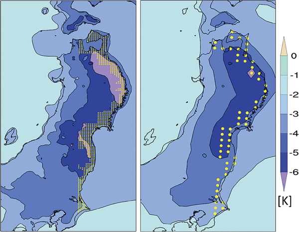
Temperature anomaly distribution from DSJRA-55 (left) and 48-member NHRCM historical ensemble (right) during ECDs from 1958 to 2010. Yellow markers represent grid points for extracting ECDs.
Comprehensive methodology of SOMs can be found in a growing number of peer-reviewed literature (e.g., Hewitson and Crane 2002; Gutowski et al. 2004; Nishiyama et al. 2007; Cassano et al. 2015), but key points are highlighted here. The primary purpose of the SOM algorithm (the SOM_PAK program is used for this study, which can be downloaded at http://www.cis.hut.fi/research/som-research) is to reduce high-dimensional data to a smaller array of characteristic patterns and arranged in a two-dimensional, visual-friendly pattern map. The term self-organizing refers to the unsupervised, iterative learning process in which the map is updated continuously without human intervention or comprehensive knowledge of the input data. However, prior understanding will aid in setting appropriate training parameters. For each input, the SOM algorithm selects a reference node (also referred to as neurons or centroids) with the smallest Euclidian distance out of all the reference nodes, and the selected node is designated as the best matching unit. The selected node and its topological neighbors are then updated toward the input vector, with nodes closest to the best matching unit experiencing the greater adjustment. This training is repeated over many iterations until the map converges to a steady state, with nodes with similar patterns residing close to one another and contrasting patterns placed further apart. Several trial-and-error runs are performed by deciding on an appropriate initialization parameter, number of nodes, neighbors that will be influenced by the input (radius), and the number of iteration steps for the learning process. For radius size, half the lowest dimension is commonly used (e.g., Nishiyama et al. 2007; Loikith et al. 2017), while the number of iterations is suggested to be at least 500 times the number of nodes in the SOM map (Kohonen 1995). In general, the higher the number of nodes, the more detailed the classification, but it may produce many nodes with little to no distinction between its neighbors in addition to longer computational time. Smaller maps provide representative groups for the most dominant features with less computing time but may dilute the variability present in the dataset, especially rare events. Choosing the right number of nodes is somewhat arbitrary, but it should balance the benefits and drawbacks of both large and small maps.
In determining the most appropriate SOM map for our study, the co-variate of quantization error (QE) and Sammon map (Sammon 1969), both standard outputs from the SOM algorithm, are examined. In short, QE represents the sum of the mean squared distance between each input and the best matching unit, while Sammon map is a two-dimensional representation of the Euclidian distances between each node. A “flat” Sammon map is preferred over a “twisted” or “folded” map, as it provides clearer relationships between neighboring nodes and a stable learning process. To determine the flatness of the map, we follow the twistedness index (TI) approach introduced by Cassano et al. (2015) to produce a quantitative value for the magnitude of Sammon map flatness. A perfectly flat map will have an index of 1, and higher values signal an unstable learning process, leading to a more distorted map (Fig. S1). Ideally, the most appropriate SOMs are those with minimal QE and TI.
For the purpose of model evaluation, we train the SOM algorithm on MSLP patterns over our analysis domain (Fig. 1) using all the JJA days (1958–2010) from a combination of JRA-55 and one randomly selected MRI-AGCM ensemble member [53 years × 92 days × (1 JRA-55 + 1 MRI-ACGM) = 9,752 days]. The synthesis of both the reanalysis and model circulations when training the SOM is a common approach when evaluating model performance (Schuenemann and Cassano 2009; Skific et al. 2009; Jaye et al. 2019). Others have used reanalysis MSLPs on its own (Wang et al. 2015; Gibson et al. 2016) to determine dominant synoptic patterns. Either method, however, was determined to be equally useful for model evaluation. Grid points with an elevation higher than 1000 m are omitted prior to SOM training, so the best matching unit is determined from synoptic-scale characteristics and not by differences in how each dataset represents complex topography.
Figure S2a shows the relationship between QE and TI dependent on node size and the number of iterations. It is seen that increasing the number of nodes will lower the QE but produces larger than desirable TI. Also, too many iterations will decrease QE but increase TI. Ten million iterations, for example, result in rapid TI increases at smaller node sizes than with lower iterations while providing only small improvements to QE compared to three million iterations. At larger nodes, we notice the greatest inter-iteration advantages in QE, with a difference of ∼ 25 at node size 360 compared to ∼ 4 at node size 15. Based on these results, we opted to train the SOMs using a 7 × 5 map (35 nodes), radius of 3, Gaussian neighborhood function, and three million iterations for model evaluation, which represent an appropriate balance of low QE and TI. Our decision is still subjective and not determined by a specific QE or TI thresholds. However, the number of nodes in the past studies range from 20 nodes to 50 nodes (Cassano et al. 2007; Johnson et al. 2008; Glisan et al. 2016; Fujita et al. 2019); so, 35 nodes are determined to be appropriate in capturing the diversity of synoptic patterns. Once the training procedure is completed, the map is then used to distinguish similar patterns from the JRA-55 and the one randomly selected MRI-ACGM ensemble. The choice of a rectangular SOM (7 × 5) orientation over a square SOM (i.e., 7 × 7 or 5 × 5) is based on Kohonen (1995), which suggests a more effective learning process for the map to reach a steady form. However, we find this to have negligible effects on our study.
To examine the impact of climate change on the synoptic circulation patterns inducing ECDs, we create a new “master” SOM, which trains the SOM using the historical, +2K, and +4K simulations for all JJA days, so a range of plausible historical and future MSLP patterns is considered (Schuenemann and Cassano 2010; Gibson et al. 2016). The SOM is trained using the same domain as that of the 7 × 5 map. For computational efficiency, the master SOM is created using 12 MRI-AGCM ensembles for historical, +2K (6ΔSST × 2 δSST), and +4K (same as +2K), for a total of 198,720 days (12 ensembles × 3 simulations × 60 years × 92 days), instead of the full 48-member ensemble. Lastly, we use 48 MRI-AGCM and NHRCM ensembles (2,880 years) to extract ECDs, as mentioned earlier, and the master SOM is used to determine preferable circulation patterns that result in ECDs. A larger SOM (15 × 13, 195 nodes) is used, with adjustments being made to the number of iterations and neighborhood radius (800,000 iterations and radius of 7), once again using QE and TI relationship as the reference (Fig. S2b). Master SOMs with many nodes have proven effective in examining variability in circulation patterns and changes to meteorological extremes using d4PDF (Ohba and Sugimoto 2020).
The SOM trained on all JJA days from the combined MSLP input of JRA-55 and MRI-AGCM (Fig. 3) produced 35 dominant circulation patterns for East Asia/North Pacific domain. The left column nodes depict differing positions of the western Pacific high, with the top left intruding northwest toward Bering/Okhotsk Sea, while the bottom left remains well southeast of the analysis domain, along with a surface low near the Bering Sea or Eurasian landmass. The right column nodes show the intensified OKH, with nodes 28 and 35 exhibiting weaker OKH relative to nodes 7 and 14, and is accompanied by a surface low near the Bering Sea and south and east of Japan (∼ 25–40°N, 130–160°E; EJL (east Japan low) hereafter). Figures 4a and 4c show the frequency of days each node is accessed for all JJA days in reanalysis and d4PDF. It reveals that the highest frequency is patterns similar to ones represented by nodes 1, 7, 29, and 35 for both JRA-55 and d4PDF. On the other hand, d4PDF shows lower frequencies in the bottom row of nodes (nodes 23 to 35) while over-producing much of the nodes on the top half of the map (nodes 1 to 21) compared to reanalysis. The right-most nodes are likely to promote Yamase winds to flow toward northern Japan, resulting in anomalously cool summer days. This is confirmed in Figs. 4b and 4d, where the percentage of ECD is among the greatest in node 35 for both the JRA-55 and d4PDF, with high percentages also seen in nodes 1, 7, and 21. Node 6 and node 28 exhibit the largest difference in frequency, but this can be likely attributed to subtle differences between MSLP that end up selecting the best matching unit of a neighboring node. We conclude that d4PDF model does an adequate job in producing JJA climatology and ECDs under similar circulation characteristics to those seen in JRA-55.
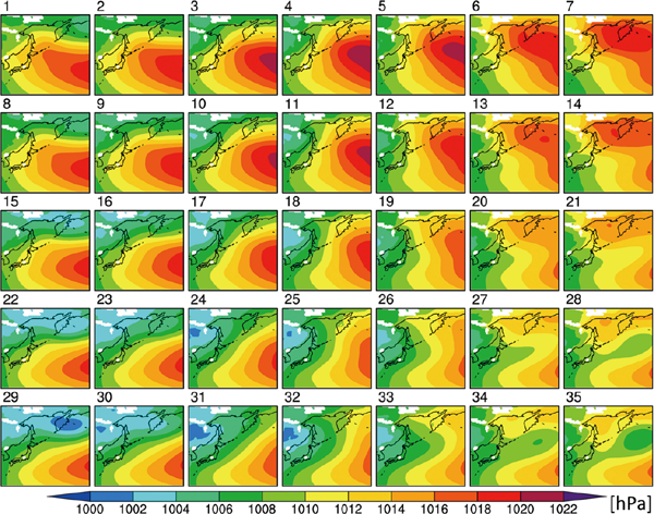
The 7 × 5 MSLP SOM of all JJA days from the combination of JRA-55 and one MRI-AGCM ensemble member. The numbers above figure indicate node number. Areas with elevation above 1,000 m are omitted before SOM training (in white from JRA-55 topography).

Frequency of MSLP patterns associated with JJA climatology and ECDs (%) for (a, b) JRA-55 and (c, d) d4PDF 48-member historical ensemble. Warmer colors represent higher frequencies. The top left number indicates node number corresponding to Fig. 3.
Figure 5 shows composites for node 35 from JJA climatology and ECDs, which is a node with among the highest ECD frequency for JRA-55 and d4PDF ensemble. Composites reveal similar intensity and location of the OKH and a strong low near the Bering Sea for both climatology and ECDs. The presence of OKH provides a more distinct couplet with the surface low to the east, allowing stronger transport of cold air from the Okhotsk Sea into the region. Tachibana et al. (2004) indicated that cold anomalies in northern Japan are not a result of OKH by itself but require a corresponding cyclonic anomaly in the northern North Pacific. This is quite clear in our results in Figs. 5 and S3. As a result, stronger cold air advection is likely enhanced through the noticeable stronger surface winds approaching northern Japan, and the lack of or weak northeasterlies like what can be seen in Figs. S4a and S4c are shown to be unfavorable in producing ECDs. These details substantiate the usefulness of SOMs in preserving vital differences between ECDs and climatology, which would have been lost if all events within each node were composited. These results may also imply that 35 nodes may not be sufficient when seeking these details. While the size of the map is still appropriate for model evaluation, as examining extremes with observations using a greater number of nodes would limit the statistical robustness for each node, utilizing the d4PDF would certainly allow for such trials to be applied. We investigate this in the next section.
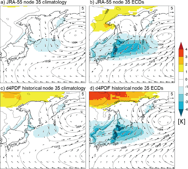
Composite of node 35 (a, b) JRA-55 and (c, d) MRI-AGCM 48-member historical ensemble of JJA climatology and ECDs. MSLP (contour, 2 hPa intervals), temperature anomaly (color, K), and 10 m near-surface winds (vectors, m s−1) are plotted. Winds vectors with speeds less than 2 m s−1 are omitted for visual clarity.
Next, we examine changes to ECDs by creating a master SOM. The master SOM (Fig. 6) shows a diverse collection of circulation patterns, ranging from strong influence from the OKH at the top right of the map, strong EJL on the bottom right, strong North Pacific high near the south of the domain on the bottom left, and a northern presence on the center-left. The larger number of nodes adds more details that were diluted by the smaller map from the model verification step (Fig. 3).

The 15 × 13 MSLP “master SOM” trained on all JJA days from historical, +2K, and +4K experiments. Black outlines indicate a cluster of nodes with the highest ECD frequency in the historical climate (Fig. 7a). MSLP and horizontal wind composites for all days are enlarged.
Figure 7a shows several nodes of preferred circulation patterns for ECDs in the historical climate using the master SOM. While many nodes show ECD occurrences, we focus on four clusters with the highest cumulative ECD frequencies. Each cluster contains four nodes, which allows them to be representative of four distinct MSLP patterns. These four clusters represent noticeable differences in synoptic circulations. ECD1 shows a dominant OKH pattern, though the center of the high is displaced slightly east of the Okhotsk Sea and toward the Bering Sea. ECD2 highlights a moderately strength OKH and a tongue of lower pressure northeastward from eastern Japan. ECD3 shows no clear OKH pattern but instead is highlighted by a strong low-pressure center near the Bering Sea, and a relatively weak North Pacific high to the south. This pattern is comparable to ECD patterns in Figs. 5b and 5d, demonstrating how a larger SOM and larger sample sizes allow us to examine characteristics such as these that would otherwise be difficult to analyze. Lastly, ECD4 shows similar features to that of ECD3, but with a stronger OKH feature.
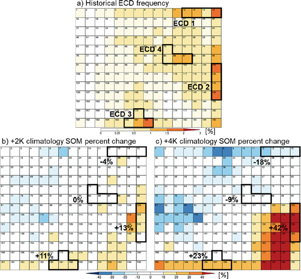
Frequency of ECD in historical (a) and percent change between the historical and the (b) +2K and (c) +4K climate experiment for all JJA days. The top left number in each box indicates node numbers. For b) and c), nodes in white indicate nodes with less than 10 % change and/or less than 4 ΔSST patterns agree on the sign of change. Black outlines indicate a cluster of nodes with the highest ECD frequency in the historical climate.
Figures 7b and 7c represent changes in node frequency in +2K and +4K JJA climatology compared to the historical ensemble, with percent change for the four ECD clusters labeled. Changes in +2K are lower relative to +4K, but both show a divide in patterns that are projected to increase or decrease in future climates. The top and left parts of the map, which are highlighted by OKH/Bering Sea high and westward expansion of the North Pacific high, respectively, show notable decreases in frequency. The projected retreat of the North Pacific high in future climates, as suggested in previous studies (He et al. 2017; Kamae et al. 2019), can be one possible reason that these patterns are projected to be less frequent in the future. The cluster at the bottom right of the map shows a considerable increase in frequency. Circulation patterns from this cluster are dominated by a low-pressure center near the southern portion of Japan and extending northeast toward the Pacific east of Japan and suggest the presence of the Baiu front. Increases in these patterns may relate to a similar onset but delayed termination of the Baiu front in future climates compared to the present (Kitoh and Uchiyama 2006; Kusunoki et al. 2006). Future changes to nodes associated with ECDs in the historical climate show ECD2 to occur much more frequently, particularly in the +4K climate. ECD1 and ECD3 show a lower decrease and increase, respectively, while ECD4 shows very little change. Lastly, it is seen that changes in dominant circulation patterns will shift gradually from historical to +2K and from +2K to +4K for most nodes.
To determine how ECDs may change beyond synoptic characteristics, we investigate the role of thermal advection in the lower troposphere during ECDs for each of the four ECD clusters for the historical, +2K, and +4K climates (Fig. 8). For each ECD cluster, differences in MSLP patterns yield different 925 hPa winds, thermal advection, and temperature anomaly distribution in northern Japan. For all historical patterns, cold air advection can be seen off eastern Japan, with the greater advection magnitudes yielding more negative surface temperatures. Also, all patterns exhibit a northeasterly wind component, allowing cooler air from the Okhotsk Sea to be transported to northern Japan. ECD1, with strong OKH features, present the weakest cold air advection among the four clusters with warmer temperature anomalies, possibly due to the contribution of warm air from the south and winds showing a more zonal flow. Another possibility may lie in the vertical structure of OKH as deep OKH, as emphasized in Tachibana et al. (2004), does not supply the necessary cold air advection that shallow OKH can provide. Changes in the structure of OKH in future climates would be of interest in further studies. The other three nodes depict strong northeasterly winds and clear boundaries from the warmer airflow from the south. These results suggest that a sharp separation between the cold air from the north and warm air to the south, either by the North Pacific high or a surface low over southern Japan, is necessary to produce strong ECDs.
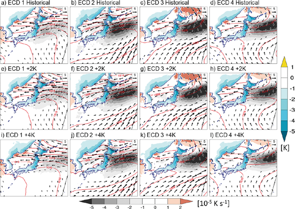
Composites of 925 hPa thermal advection (shading over water, bottom label bar), 925 hPa horizontal wind vectors (winds over land and speeds less than 2 m s−1 is omitted), MSLP (red contours, 2 hPa intervals), and surface temperature anomaly (shading over land, right label bar) from the four high-frequency ECD nodes (Fig. 7a) for the historical, +2K, and +4K NHRCM experiments.
Future changes reveal gradual warming of ECDs associated with weaker cold air advection. To examine the cause of the weakening cold air advection, we investigate the changes in horizontal wind and meridional temperature gradient components of thermal advection (Fig. 9). We note here that the zonal temperature gradient was examined but did not exhibit significant changes. Future patterns reveal little to no change in winds, particularly in the region with strong cold air advection. We do see, however, a positive change in meridional temperature gradient near the area of a strong negative meridional gradient. While these features are less clear in the +2K compared to +4K (which results in limited ECD change at the surface), this would imply a weaker meridional temperature gradient in future climates and results in warmer ECDs compared to historical climate. Interestingly, this is consistent between all ECD clusters, which seems to suggest that while ECDs may continue to persist, they may be warmer than ECDs in present-day climate.

Future changes in surface temperature anomalies (shading over land, vertical label bar), 925 hPa horizontal winds (vectors, m s−1, speeds less than 0.5 m s−1 omitted), and meridional temperature gradient (shading over water, horizontal label bar) in +2K and +4K climate from the four high-frequency ECD nodes. Blue contour lines show meridional temperature gradients less than −0.6 × 10⁻⁵ K s−1 in the historical climate. Only changes significant at the 95 percent confidence interval by the student t-test is plotted.
There are important caveats with this study worth mentioning. Perhaps the greatest influence on ECDs in northeast Japan would be from the SST characteristics surrounding the Sanriku coast (Fig. 1). Kodama (1997) revealed that local SSTs can substantially transform low-level cloud development, primarily through differences from atmospheric mixed/stable layer contributions. As described in Section 2, d4PDF future ensembles rely on six ΔSST patterns from CMIP5, and Sanriku coast (along with the Okhotsk Sea) has been shown to exhibit large intermodel spread in SSTs (Zhou and Xie 2017), a distinction also confirmed for ΔSST utilized in d4PDF (not shown). To ensure each SST contributes an equal fraction of future ECDs, we calculated temperature anomalies on a per-ΔSST basis. If we extracted the 5th percentile from the entire +4K ensemble (48 members) instead of how it was defined in this study, ∼ 31 % of the total ECDs were from the HadGEM2-AO ΔSST, and only ∼ 10 % are from the MPI-ESM-MR, with similar percentages seen in the +2K climate. This can be attributed to the propensity for certain ΔSSTs to develop low-level clouds, particularly near the Sanriku coast, at much higher fractions (HadGEM2-AO) than others (MPI-ESM-MR) in future simulations. Finally, while the influence of low-level clouds to SST on a daily timescale may be insignificant, persistent Yamase type events may act to lower SSTs (Kodama et al. 2009), which could be an important teleconnection not captured by atmosphere only GCMs.
This study takes advantage of both the d4PDF's ability to produce large samples of extreme events and pattern segregation techniques using SOMs to evaluate variability in synoptic circulation patterns and how climate change may impact extreme events. Preliminary examination of ECDs, defined as days with widespread temperature anomalies less than the 5th percentile, was examined using SOMs. Two different maps, one for climate model evaluation and one for evaluating the near-future and end-of-century projected changes, were created using MSLP patterns in an East Asia/North Pacific domain.
In the model evaluation step, SOMs were trained on all JJA MSLPs from the JRA-55 and one MRI-AGCM ensemble member, and the same map was used to determine the frequency of DSJRA-55 and NHRCM ECDs corresponding to the representative circulation fields produced by SOMs. While some variability exists, the MRI-AGCM ensemble captured the preferred synoptic field during ECDs seen in the JRA-55. Further validation was performed by compositing MSLP, temperature anomalies, and surface winds for several nodes representing the highest ECD frequencies. The location and intensity of the OKH are well represented in the models, as is the surface low characteristics near the Bering Sea or off eastern Japan. Additionally, composites of climatology and ECD on nodes with highest frequency ECDs reveal differences in characteristics, such as stronger high-pressure center north of Hokkaido and stronger northeasterlies approaching northern Japan.
For future climate evaluation, we created a new “master” SOM, training a combined MRI-AGCM historical, +2K, and +4K MSLP fields for all JJA days. The master SOM map provided additional circulation patterns than the map used in model evaluation and was useful in investigating future changes in greater detail. MSLP patterns inducing ECDs show a clear transition of increased and decreased nodes, with patterns showing the presence of a strong OKH/Bering Sea high and westward extent of the North Pacific high decreasing in +2K, and more so in the +4K climate. Increases in frequency were significant for patterns dominated by surface low pressure in southern Japan toward offshore of eastern Japan paired with a moderately strong OKH. Lastly, we examined how the specific circulation patterns during ECD that are largely unchanged between historical and future climates alter the underlying surface characteristics and the possible mechanisms behind it. It is suggested that differences in thermal advection play a major role in surface temperature variability and that similar synoptic patterns will not necessarily result in similar magnitudes of cold air advection. For future changes, a weakening of cold air advection, particularly in +4K, was found to be largely due to a weakening meridional temperature gradient, regardless of circulation patterns. This resulted in weaker ECDs, indicating the possibility that while ECD will undoubtedly occur in future climates, they may not be as cool as what is experienced at present. While changes in temporal distribution and duration of ECD need to be taken into consideration, these results are notable.
Figure S1. A 20 × 18 Sammon map example of a) flat and b) twisted orientation.
Figure S2. Twistedness index (dashed lines) and quantization errors (solid lines) versus the number of nodes with a different number of iterations for a) JRA-55 + MRI-AGCM SOM and b) historical, +2K, and +4K master SOM. Learning rate (0.01), neighborhood function (Gaussian), shape of SOM (rectangular), and radius (approximately half of the smallest dimension) is consistent for both SOMs.
Figure S3. Same as Fig. 5, but for node 7.
Figure S4. Same as Fig. 5, but for node 1.
This study was supported by the Social Implementation Program on Climate Change Adaptation Technology (SI-CAT) and the Environment Research and Technology Development Fund JPMEERF20192005 of the Environmental Restoration and Conservation Agency of Japan. The Earth Simulator supercomputer was used in this study as part of the “Strategic Project with Special Support” of JAMSTEC. The study was also supported by the Program for Risk Information on Climate Change (SOUSEI) and the Data Integration and Analysis System (DIAS), both of which are sponsored by the Ministry of Education, Culture, Sports, Science and Technology of Japan. (MEXT). The d4PDF dataset available at (https://www.diasjp.net/). We would like to thank the organizers of the annual “Yamase colloquium”, which sparked many insightful discussions with its participants that helped motivate this study. Lastly, we thank the editor (Tomonori Sato) and the two anonymous reviewers for their valuable insights, which significantly improved the quality of this manuscript.