９月の発達した低気圧によるシベリアから北極域への黒色炭素エアロゾル輸送に対するモデル分解能の影響

Abstract

Atmospheric transport of aerosols such as black carbon (BC) affects the absorption/scattering of solar radiation, precipitation, and snow/ice cover, especially in areas of low human activity such as the Arctic. The resolution dependency of simulated BC transport from Siberia to the Arctic, related to the well-developed low-pressure systems in September, was evaluated using the Nonhydrostatic Icosahedral Atmospheric Model–Spectral Radiation Transport Model for Aerosol Species (NICAM-SPRINTARS) with fine (∼ 56 km) and coarse (∼ 220 km) horizontal resolutions. These low-pressure systems have a large horizontal scale (∼ 2000 km) with the well-developed central pressure located on the transport pathway from East Asia to the Arctic through Siberia. In recent years, the events analysis of the most developed low-pressure system indicated that the high-BC area in the Bering Sea observed by the Japanese research vessel Mirai on September 26–27, 2016, moved to the Arctic with a filamental structure from the low's center to the behind of the cold front and ahead of the warm front in relation to its ascending motion on September 27–28, 2016. The composite analysis for the developed low-pressure events in September from 2015 to 2018 indicated that the high-BC area was located eastward of the low's center in relation to the ascending motion over the low's center and northward/eastward area. Since the area of the maximum ascending motion has a small horizontal scale, this was not well simulated by the 220-km experiment. The study identified that the BC transport to the Arctic in September is enhanced by the well-developed low-pressure systems. The results of the transport model indicate that the material transport processes to the Arctic by the well-developed low-pressure systems are enhanced in the fine horizontal resolution (∼ 56 km) models relative to the coarse horizontal resolution (∼ 220 km) models.

1. Introduction

The emission and transport of black carbon (BC) aerosols are essential factors that influence our understanding of air pollution, solar radiation, and precipitation prediction. BC efficiently absorbs solar radiation, influences the heating of the atmosphere and the melting of sea ice and snow (Myhre et al. 2007), and indirectly influences cloud microphysics (Ackerman et al. 2000). In areas of low human activity such as the Arctic, even a small inflow of BC aerosols can directly and indirectly influence solar radiation, clouds, and precipitation (Quinn et al. 2008; Sand et al. 2016), making it important to better understand BC transport to the Arctic. BC is emitted into the atmosphere by anthropogenic and biomass burning sources, which is thought to be transported to the Arctic in winter, spring, and autumn from anthropogenic sources and in summer from biomass burning sources (Stohl 2006; Matsui et al. 2011; Ikeda et al. 2017). These studies revealed that primary BC sources transported to the Arctic are anthropogenic emissions in Asia, Europe, Russia, and North America and biomass burning emissions in Siberia, Alaska, and Canada.

The current models have a large variability in the radiative forcing of the BC due to diversity in the simulated vertical profile of BC mass, especially above 5 km (Samset et al. 2013). Di Pierro et al. (2011) indicated that the pollution plumes detected in the middle troposphere by the Cloud-Aerosol Lidar with Orthogonal Polarization onboard the Cloud-Aerosol Lidar and Infrared Pathfinder Satellite Observations were transported from East Asia to the Arctic through eastern Siberia. The vertical profile from the surface to 7 km of aircraft (WP-3D) observations operated by the National Oceanic and Atmospheric Administration also indicated that the BC mass mixing ratios peaked at around 5 km in the middle troposphere (Spackman et al. 2010). The Goddard Earth Observing System (GEOS)-Chem simulation by Ikeda et al. (2017) also indicated that the BC emitted from East Asia was transported to the Arctic mainly over the Sea of Okhotsk and eastern Siberia in the middle troposphere. Ikeda et al. (2017) also indicated that a strong input of East Asia BC to the Arctic went through the “window area” over 130–180°E and 3–8 km, crossing the latitude of 66°N. The findings show that since the same isentropic layer in higher latitudes is located in higher altitudes than in midlatitudes, the anthropogenic BC emitted from East Asia is transported to the Arctic at relatively high altitudes and that BC in higher altitudes is transported to lower altitudes through vertical mixing in the Arctic (Ikeda et al. 2017). The global lifetime of BC is about a week (IPCC 2013; Lee et al. 2013), while the BC lifetime in the Arctic is about 20 days (Mahmood et al. 2016) and that for BC originating in East Asia is about 60 days, due to it being distributed in the middle troposphere (Ikeda et al. 2017).

Although storm activities peak over the midlatitude oceans in winter (e.g., Blackmon et al. 1977), there is a relative maximum in storm frequencies during summer over northern Eurasia at 60–70°N, especially around Siberia, due to the summer baroclinic zone along the coastline of the Arctic Ocean (Serreze et al. 2001). The pattern of the storm activities in September is similar to that in the summer. Hence, the well-developed low-pressure systems are likely located in the aforementioned “window area” in September. This implies that the storm determines the BC transport from East Asia/Siberia to the Arctic in September and should be well reproduced by models to properly estimate the BC impacts on the Arctic climate. Therefore, a dedicated study evaluating the modeling capability regarding transport associated with such a low-pressure system in this geographical region is required.

To evaluate the capability of simulating the transport process around the low-pressure systems, we used the Nonhydrostatic Icosahedral Atmospheric Model (NICAM)–Spectral Radiation Transport Model for Aerosol Species (SPRINTARS). The horizontal resolution of ∼ 200 km is commonly used in long-term climate simulations with a global aerosol transport (e.g., Myhre et al. 2013). We used a fine horizontal resolution of 56 km, which is the finest level among state-of-the-art models for long-term climate simulations with aerosol components. This resolution is capable of simulating fine-scale transport processes such as the accumulation of mass behind cold fronts (Ishijima et al. 2018) and the wet deposition process around low-pressure systems (Sato et al. 2016). The frontal structure around the low-pressure system in a coarse-resolution model (∼ 220 km) is not well resolved (Ishijima et al. 2018), implying that the transport process around a low-pressure system, such as the upward motion around the warm front, is also not sufficiently resolved/reproduced in the coarse-resolution model. The upward motion has a small horizontal scale variability, whereas a large scale of south-to-north movement in front of the low-pressure system is required to represent the whole BC transport from the midlatitude into the Arctic. In other words, sufficient representation of transport associated with such a low-pressure system in the models requires a large horizontal domain (∼ 2000 km) as well as a fine grid to resolve the structure in the upward motion and the well-developed central pressure. We used the recent fine horizontal resolution (56 km) of Nonhydrostatic Icosahedral Atmospheric Model–Spectral Radiation Transport Model for Aerosol Species (NICAM-SPRINTARS) comparing with the coarse horizontal resolution (220 km) to evaluate the resolution dependency of the vertical BC transport around the low-pressure system as well as the wet deposition and accumulation of BC behind cold fronts.

The novelty of this study is to investigate the resolution dependency of the BC transport from Siberia to the Arctic in relation to the well-developed low-pressure systems in September.

The rest of this paper is structured as follows. Section 2 presents data and methods, including the description of the model. Section 3 discusses the validation of the model experiments, and Section 4 presents BC transport by the low-pressure system. Finally, Section 5 presents the conclusions.

2. Data and methods

2.1 Observations

For evaluating the capability of simulating BC aerosols in the global aerosol transport model, we used the BC mass concentration data at a ship-based and ground-based observation in September 2016 when significant aerosol emissions originated as a result of a major forest fire near Lake Baikal, Russia.

For the ship-based observation data, the surface BC were observed on the research vessel (R/V) Mirai of the Japan Agency for Marine-Earth Science and Technology, from August 22, 2016 to October 6, 2016, by around trip from ports of Hachinohe (40.55°N, 141.53°E), Japan, to the Arctic Ocean through the Northwestern Pacific and Bering Strait as an Arctic Ocean research cruise (MR16-06). The BC concentration was measured by the single-particle soot photometer (SP2; Droplet Measurement Technologies, Inc., USA) (Taketani et al. 2016; Miyakawa et al. 2016, 2020). The observed particle size range was 80–500 nm (mass equivalent diameter). The BC concentration we used in this study was estimated by the same protocol used by Taketani et al. (2016).

The surface BC concentration was continuously observed by the multi-angle absorption photometers (MAAP; model 5012, Thermo Fisher Scientific, Inc., USA) on Fukue Island (red diamond in Fig. 2, 32.75°N, 128.68°E; 75 m above sea level), western Japan (Kanaya et al. 2013, 2016; Miyakawa et al. 2019). This observation site is located on the downstream of significant source regions in East Asia, with no significant emission sources around the observation site.

Fig. 1.

Surface weather chart near the Aleutians at (a) 12:00 UTC on September 25, and (b) 12:00 UTC on September 26 (Japan Meteorological Agency, https://www.jma.go.jp). Blue arrows indicate the location of R/V Mirai; the marker is enlarged and shown in the lower right panels.

Fig. 2.

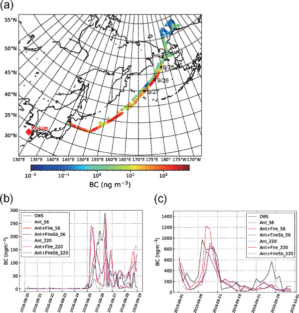
(a) Course of R/V Mirai and surface BC concentration (ng m⁻³). The locations at 00 UTC for September 25–27 are denoted by crosses. The red diamond indicates the location of Fukue Island. (b) Time series of hourly surface BC concentration along R/V Mirai's track for September 20–28 (black line, observation; red lines, Ant+ Fire; gray lines, Ant; purple lines, Ant+FireSb). Solid (dashed) lines indicate 56-km and 220-km experiment results. (c) Time series of daily mean surface BC concentration at Fukue Island in September 2016.

To evaluate the precipitation of the model, we used the daily Global Precipitation Climatology Project (GPCP), v.1.3 (Huffman et al. 2001; Adler et al. 2017), which can be accessed via the National Centers for Environmental Information website (https://www.ncei.noaa.gov). The vertical flow of the model was evaluated with the Japanese 55-year Reanalysis (JRA-55) project conducted by the Japan Meteorological Agency (JMA) (Kobayashi et al. 2015), and the dataset can be accessed via the JMA website (https://jra.kishou.go.jp/).

2.2 Model

a. General description

The NICAM (Tomita and Satoh 2004; Satoh et al. 2008, 2014) combined with the SPRINTARS (Takemura et al. 2000, 2002, 2009; Goto et al. 2011) was developed to calculate global aerosol transport and its influences on radiation and precipitation (Suzuki et al. 2008; Goto et al. 2015). The NICAM-SPRINTARS simulates the mass concentration of primary tropospheric aerosols such as carbonaceous aerosols [BC and organic carbon (OC)], sulfates, sea salt, and dust, along with their emissions, transport, and dry/wet deposition processes. If there are cloud particles in the model grid area, a part of the aerosol particles is assumed to be in the cloud particles, and the rest is assumed to be in the surrounding atmosphere. The ratio of in-cloud and interstitial aerosols is fixed in the model (Takemura et al. 2000). In the wet deposition process of this model, in-cloud-aerosol particles are assumed to be removed by precipitation (“rainout”), and the interstitial particles are assumed to be removed by collision with precipitation particles (“washout”). The rainout is calculated with cloud to rain conversion rate and cloud fraction, and the washout is calculated with precipitation flux. In this model, sulfate aerosols were formed from their precursor, sulfur dioxide (SO₂). For the BC, three independent variables were introduced, namely, BC from biomass burning as a result of forest fires, hydrophilic BC from anthropogenic emission, and hydrophobic BC from anthropogenic emission. The BC originating from forest fires was assumed to be hydrophilic. Half of anthropogenic BC was assumed to be hydrophobic in its emission stage, and there was no conversion process from hydrophobic to hydrophilic. The setting for ratio of hydrophobic to hydrophilic may change the amount of BC inflow to the Arctic. However, those assumptions could not change the conclusion that the BC transport to the Arctic by the well-developed low-pressure systems is enhanced in the fine horizontal resolution (∼ 56 km) models relative to the coarse horizontal resolution (∼ 220 km) model. Note that we used a 0.1° × 0.1° longitude–latitude original resolution of the anthropogenic emission sources in 2010 from Emission Database for Global Atmospheric Research Hemispheric Transport of Air Pollution (EDGAR-HTAP) v2.2 emission inventory (Janssens-Maenhout et al. 2015).

Veira et al. (2015) reported that the implementation of a specific plume height parameter slightly reduces the model bias around an aerosol emission area. Thus, we improved the plume height parameterization of NICAM-SPRINTARS by replacing the original model's globally uniform injection height (∼ 3 km) with an estimated injection height for the forest fire's pyro-convection. The emission flux was uniformly partitioning with its mixing ratio into the levels from the surface to the injection height for both the original and improved versions of the model. To simulate the high temporal variation of emissions at daily time scales, we used the daily dataset of the Copernicus Atmosphere Monitoring Service (CAMS) Global Fire Assimilation System (GFAS) provided by the European Centre for Medium-Range Weather Forecasts for wildfire-related fluxes of BC, OC, and SO₂, along with the mean altitude of maximal injection as estimated from the NASA Terra Moderate Resolution Imaging Spectroradiometer (MODIS) and Aqua MODIS satellite observations. The original resolution of the GFAS is a grid of 0.1° × 0.1° longitude–latitude resolution. When comparing the 56- and 220-km simulations, the emission flux and mean altitude of maximal injection of the 220-km resolution were converted to the 56-km resolution to ensure the same emission and injection height for both resolutions.

b. Experimental setup

The NICAM-SPRINTARS used in this study had 78 vertical layers from the surface to ∼ 50-km altitude. The vertical thickness at the planetary boundary layer was about 100–200 m, reaching about 400 m for 3.5–18 km. To analyze the horizontal sensitivity, we performed simulations using 56-km and 220-km horizontal resolutions. Both 56-km and 220-km resolutions use the same cumulous parameterizations and parameters (Chikira-scheme; Chikira and Sugiyama 2010) of NICAM.

First, a 10-year spin-up run with the 220-km model was performed to stabilize the soil moisture of the surface model MATSIRO (Minimal Advanced Treatments of Surface Interaction and RunOff), described in Takata et al. (2003). Next, hindcast simulations with both resolutions were performed, since the model's meteorological fields needed to be similar to those of the real atmosphere for the aerosol transport simulations. For the hindcast simulations, the meteorological fields were nudged toward those recorded in the dataset of the National Centers for Environmental Prediction (NCEP)-Final (FNL) operational reanalysis, using the 6-h interval data of zonal and meridional winds along with the temperature, and all the vertical levels of NCEP-FNL data were converted to the model levels. The NCEP-FNL has a 1° × 1° longitude–latitude resolution. The model's sea surface temperature was prescribed by weekly interval data from the Optimum Interpolation Sea Surface Temperature (OISST) V2.

In order to evaluate the capability of simulation of the BC peak event around the developed low-pressure system on September 25–26, 2016, we performed various sensitivity experiments starting from July 1, 2016 (Table 1). One control experiment included the presence of anthropogenic emissions along with the global fire activity (Ant+Fire), another experiment included only the former (Ant), and the third experiment evaluated the effect of the emissions from the Siberian forest fire in conjunction with anthropogenic emissions (Ant+FireSb). The fourth experiment assessed the effect of wet deposition of BC by precipitation by excluding the wet deposition process (Ant+FireSb_NOWDEP).

To evaluate the general transport process around the developed low-pressure systems in September, we performed long-term hindcast simulations of both 56-km and 220-km horizontal resolutions. Owing to the limitation of computational resources, only the control experiment (Ant+Fire) was performed from January 1, 2015 to December 31, 2018.

3. Validation of the model experiments

Dai et al. (2014) validated the seasonal evolution of the 550-nm aerosol optical thickness, the 440- and 870-nm Ångström exponent, and the 550-nm single scattering albedo of NICAM-SPRINTARS, compared with the observational products from the MODIS and the Aerosol Robotic Network (AERONET). Whereas Goto (2014) and Goto et al. (2015) validate the surface concentrations of the simulated BC by NICAM-SPRINTARS in Asia, in this study we validated the surface concentration, transport process, and wet deposition process of the BC in this model.

3.1 BC concentrations at ship-based and ground-based observation

The BC concentrations along R/V Mirai's track were identified a peak event on September 25–26, 2016, which was suggested to be influenced by forest fire. At the same time, the most developed low-pressure system as the minimum sea level pressure (SLP) in recent years, which reached the polar region (> 60°N) through the “window area”, was observed around R/V Mirai's track. This low-pressure system, which was observed above the Sea of Okhotsk at 12:00 UTC on September 25, 2016 (Fig. 1a), moved to the polar region at 12:00 UTC on September 26, 2016 (Fig. 1b). The vessel was located ahead of the warm front at 12:00 UTC on September 26 and observed southwesterly winds (Fig. 1b) of the low-pressure system, implying the movement of the BC-rich air to the Arctic. In this study, this event was used to evaluate the capability of a global aerosol transport model in simulating the long-range (several thousand miles) transports to the Arctic, in terms of transport pathways, deposition processes, and resolution dependency (56 km vs. 220 km).

The surface BC concentration along R/V Mirai's track showed a maximum of ∼ 290 ng m⁻³ on September 26 and a mean of ∼ 110 ng m⁻³ on September 25–26 in the Bering Sea which continuously enhanced for those 2 days (Fig. 2b and Table 2). The BC concentration for Ant+Fire_56 showed one peak event on September 25 and two peak events on September 26. The first peak on the 26th (∼ 270 ng m⁻³) was similar to that observed in terms of timing and maximum concentration, while other peaks were overestimated. In contrast, Ant+Fire_220 showed low concentration peaks (∼ 150 ng m⁻³ on the 25th and ∼ 120 ng m⁻³ on the 26th) relative to Ant+Fire_56 with slow temporal changes on those 2 days. Although continuous enhancement on the 25th and 26th was not simulated in the model, the mean concentrations were reproduced by both Ant+Fire_56 (∼ 90 ng m⁻³) and Ant+Fire_220 (∼ 80 ng m⁻³). The relative importance of anthropogenic and fire sources was examined based on the Ant, Ant+Fire, and Ant+FireSb experiments. Without considering any fire emissions (Ant), the maximum/mean of the BC concentration on September 25–26 was much smaller than the observed concentrations, indicating a minor contribution from anthropogenic BC. In comparison, both Ant+FireSb and Ant+Fire agreed with the observed maximum/mean BC on September 25–26, suggesting that these BC concentrations mainly originated from the Siberian forest fire.

Figure 2c shows the daily time series of the surface BC concentration at the observation site of Fukue Island in September 2016. Although the model experiments underestimated a peak at 25th, a peak is well reproduced around 10th, and lower values are reproduced around 15th. The relative importance of the anthropogenic source was significant for this site, and the time evolution in the 220-km resolution is vague compared with the 56-km resolution.

3.2 Transport process of the Siberian forest fire BC to the Bering Sea

To evaluate the improved plume height parameterization for wildfire-related fluxes, we focused on the large emission event that occurred as a result of a major forest fire near Lake Baikal in September 2016 (Fig. 3). Figure 4 shows the daily mean values of column BC densities from fire emissions, which were estimated by the subtracting the Ant+FireSb_56 outputs from the Ant_56 outputs. Ant+FireSb calculates the BC emissions from the Siberian forest fire over the region within 90–140°E and 50–70°N (green rectangle in Figs. 3, 4); thus, the impact of the Siberian fire could be derived from the model outputs. This high-BC area originated near Lake Baikal in Siberia around September 21–22, 2016, and was transported to the Bering Sea via Yakutsk on the 23rd (orange rectangle), the Kamchatka Peninsula on the 24th (cyan rectangle), and the Bering Sea on the 25th–26th (blue rectangle). It is noteworthy that precipitation in the low-pressure system within/around the high-BC area occurred near Yakutsk on the 23rd, the Kamchatka Peninsula on the 24th, and the Bering Sea on the 25th.

Fig. 3.

Monthly mean emission flux of BC (shading, × 10⁻¹¹ kg m⁻² s⁻¹) in September 2016 from CAMS GFAS.

Fig. 4.

Daily mean values of column BC densities (shading, µg m⁻²) estimated by the subtraction of Ant_56 from Ant+FireSb_56 on September 21–26.

In order to trace the daily movements of the air parcel with a high-BC concentration from the fire emissions, we calculated the area mean column BC densities from 50°N to 70°N for four longitudinally binned areas with a width of 50° (Fig. 5a) from region 1 (Siberia) on the 21th–22nd, to region 2 (Yakutsk) on the 23rd, region 3 (the Kamchatka Peninsula) on the 24th, and finally to region 4 (Bering Sea) on the 25th–26th. This procedure would estimate the apparent BC flow across the boundary of each region in case of a discrepancy between the movement of the averaged region and the actual movement of the BC. Figure 5b shows the time series for the column BC. Near Lake Baikal on September 22, the column BC was about 650 µg m⁻² for Ant+FireSb (Table 3). On September 26, this decreased exponentially to about 60 µg m⁻² in the Bering Sea. The cumulative precipitation was calculated by the accumulation of the area mean daily precipitation over the same area in the column BC. The cumulative precipitation (starting from the 21st) increased from the 22nd–25th, reaching ∼ 10.4 mm for Ant+FireSb_56 and ∼ 9.0 mm for Ant+FireSb_220, respectively, in agreement with the timing of the decline in column BC. Without the wet deposition of BC (Ant+FireSb_NOWDEP), there was no exponential decline in column BC, suggesting that the wet deposition of BC mainly caused the rapid decline of column BC during the transport from Siberia to the Bering Sea.

Fig. 5.

(a) Regional numbers for the area means. (b) Daily time series of the area means for column BC densities (µg m⁻²) calculated for 50–70°N and every 20° of longitude along with the air parcel movement (red lines, Ant+ FireSb; blue lines, Ant+FireSb_NOWDEP; solid lines, 56-km experiments; broken lines, 220-km experiments), estimated by the subtraction of the Ant outputs. Aqua lines indicate cumulative precipitation (mm) in Ant+FireSb.

Kanaya et al. (2016) estimated that the accumulated precipitation along trajectory (APT) is about 15 mm to reach half value of BC transport efficiency (TE) using the observed concentrations of BC and CO at Fukue Island. The CO concentrations were not simulated in this model, and then the BC results of Ant+FireSb_NOWDEP (BC_NOWDEP) are assumed to be the non-changeable tracer by wet deposition as   

The APT values of about 6 mm and 4 mm are needed to reach half the value of BC TE for 56-km and 220-km resolutions, respectively. Although the method of estimation and the target area are different from those in Kanaya et al. (2016), the estimated values of model's TE might be more sensitive to precipitation than observation. In addition, Kanaya et al. (2016) used the surface BC to estimate the TE, while our study used the column BC.

The global BC lifetime estimated by column BC and wet deposition flux in September is 6.4 days for Ant+FireSb_56 and 7.2 days for Ant+FireSb_220, in agreement with the global BC lifetime of about 1 week by IPCC (2013), indicating the removal processes of BC are realistically simulated in this model.

3.3 Precipitation of the model

To evaluate the spatial distribution of the precipitation and estimate the wet deposition, we calculated the cumulative precipitation and wet deposition flux from September 21–23 (Fig. 6), when the high-BC area was located within regions 1 and 2 (90–160°E, 50–70°N; gray rectangle in Fig. 6). Patchy peak precipitation areas were seen around Siberia (red circles) based on the data from the daily GPCP. Similar patchy peak precipitation areas were reproduced by Ant+ FireSb_56, indicating similar patterns of wet deposition flux from northeast of Lake Baikal to Kamchatka. In contrast, a single large peak area of wet deposition flux was present for Ant+FireSb_220 due to the larger precipitation area when using a coarse resolution model. Although the cumulative precipitation in Ant+ FireSb_220 was smaller compared with that in Ant+ FireSb_56 (Fig. 5), this larger precipitation area in Ant+FireSb_220 can widely enhance the decline in BC, indicating the similar decline rates between Ant+ FireSb_56 and Ant+FireSb_220. Note that similar results were derived from Ant+Fire_56 and Ant+Fire_220 (not shown). These results are comparable with the mean concentrations observed in the Bering Sea (Table 2).

Fig. 6.

Cumulative precipitation (mm) from September 21–23: (a) for the GPCP, (b) for Ant+Fire_56, and (c) for Ant+Fire_220. (d–e) Cumulative wet deposition flux of BC (mg m⁻²).

4. BC transport by low-pressure systems

4.1 Developed low event in late September 2016

a. High-BC area linked to the weather on September 25–26, 2016

Figure 7a shows the surface BC concentrations of Ant+FireSb_56 at 12:00 UTC on September 25 and 12:00 UTC on September 26, together with the SLP. Compared with the surface weather chart presented in Fig. 1, Ant+FireSb_56 well reproduced the location and central pressure of the low-pressure system in the Sea of Okhotsk at 12:00 UTC on September 25, 2016, and the polar region around the Kamchatka Peninsula at 12:00 on September 26, 2016. This low-pressure system was accompanied by a cold and a warm front (Fig. 1). The filamental structure of the high-BC area is visible from the low's center to behind the cold front and ahead of the warm front, elongating to another low-pressure system in the Bering Sea. Although the low-pressure system in the Bering Sea had no associated frontal system in the surface weather chart, the high-BC area was continually shown between the two low-pressure systems, suggesting that the frontal structure was located between these two low-pressure systems.

Fig. 7.

Snapshots of surface BC concentrations (shading, ng m⁻³) from (a) Ant+FireSb_56 and (b) Ant+FireSb_220. Black lines indicate SLP (thin, every 4 hPa; thick, every 20 hPa). Blue square denotes the location of R/V Mirai.

The low-pressure systems in the Bering Sea and the Sea of Okhotsk were relatively weak, with the widespread low center in Ant+Fire_220 (Fig. 7b). Moreover, the high-BC area between the two low-pressure systems was relatively widespread and lower in magnitude as the frontal structure was not well simulated in the 220-km resolution. The passage of the high-BC area ahead the warm front of a low-pressure system in the Bering Sea occurred before 12:00 UTC on September 26. The surface BC concentration along R/V Mirai's track showed an increase in magnitude ∼ 100 ng m⁻³ during several hours before the peak event and a decrease in magnitude to ∼ 10 ng m⁻³ during several hours after the peak event (Fig. 2b). Although continuous enhancement during the 25th and 26th was not simulated in the model for both the 56-km and 220-km resolutions, the sharp increase/decrease of the BC concentration was reproduced around the peak in the 56-km resolution only. The difference in the BC concentration at the frontal structure between the 56-km and 220-km simulations was consistent with that derived from the radon-222 variability being larger amount in 14–56 km than ∼ 220 km (Ishijima et al. 2018).

b. BC transport to the Arctic, September 27–28, 2016

To evaluate the BC transport to the Arctic related to the developed low-pressure system following the event described in Section 4.1a, we analyzed the temporal variation of BC concentration for the Ant+FireSb_56 experiment (Fig. 8a). The low-pressure system in the Sea of Okhotsk at 12:00 UTC on September 25 (Fig. 7a) moved to the Arctic at 00:00 UTC on September 27, with its central pressure at about 980 hPa around 160°E, 70°N. This remained almost constant, with a large horizontal scale (i.e., the length of SLP < 1000 hPa range larger than ∼ 2000 km), until 12:00 UTC on 28th (Fig. 8a). The elliptic axis of closed contours around the center of the low-pressure system was in the north–south direction at 00:00 UTC on September 27 (blue dotted line) and rotated counterclockwise toward the northwest–southeast direction at 12:00 UTC on September 27, the west–east direction at 00:00 UTC on September 28, and the southwest–northeast direction at 12:00 UTC on September 28. These axes were accompanied by the filamental structure of the high-BC area, which was transported to the Arctic with the counterclockwise rotation of the axis. Note that there were two filamental structures of the high-BC area along the 170°E and 180°E meridians at 00:00 UTC on September 27, which merged into a single filamental structure at 12:00 UTC on September 28, due to the change in frontal systems. A similar filamental structure of the high-BC area was simulated at the height levels from 850 hPa to 500 hPa (Figs. 8b–d), and the BC concentration decreased with an increase in the height level. Even for the 400-hPa level, the filamental structure showed a small magnitude (Fig. 8e), elongated from the center of the low-pressure system to the midlatitude, especially along the warm front in the Bering and Chukchi Seas on September 27 and Alaska on September 28. These results suggest that BC transport into the Arctic is related to the upward and south-to-north movement in front of the well-developed low-pressure system with a large horizontal scale.

Fig. 8.

The same as Fig. 7, but for (a) surface, (b) 850 hPa, (c) 700 hPa, (d) 500 hPa, and (e) 400 hPa of Ant+Fire_Sb_56 from 0:00/12:00 UTC on September 27–28.

For the Ant+FireSb_220 experiment, the axis of the low-pressure system was not clear, and the high-BC area was widespread, with a relatively smaller amount of maximum concentration (Fig. 9a). In addition, there was no significant high-BC area (> 5 ng m⁻³) north of 75°N from the surface to 500 hPa and north of 65°N for 400 hPa (Figs. 9b–e). Moreover, a high-BC area along with the frontal structure was not clear above 700 hPa, suggesting a weak BC transport around the low-pressure system and the front line.

Fig. 9.

The same as Fig. 8, but for Ant+FireSb_220.

Figure 10 shows the vertical p-velocity at 700 hPa, which is usually used as a diagnostic of the vertical motion around the low-pressure system and the front line. The upward motion on September 27 based on the JRA-55 dataset is significant, with its minimum at about −300 hPa d⁻¹ in the Arctic at 160°E, 70–75°N over the surface low-pressure system, accompanied by the upward motion area from the Arctic to the Bering Sea around 180°E meridian (Fig. 10a). The results of Ant+FireSb_56 indicate a similar pattern, with a comparable magnitude (Fig. 10c). This upward motion area corresponds to the high-BC area from the surface to the 400-hPa level, along with the frontal structure (Fig. 8), indicating a significant contribution from the vertical transport of the BC by the ascending motion around the low-pressure system involved in the south-to-north transport. This ascending motion area is moved to Alaska from around 180°E to around 160°W meridian on September 28 (Figs. 10b, d), corresponding to the movement of the frontal structure around the low-pressure system. In contrast, the magnitude of the ascending motion for Ant+FireSb_220 is small (minimum about −100 hPa d⁻¹) (Figs. 10e, f), corresponding to the small concentration of BC in upper altitudes due to the weak transport. The resolution difference in the vertical velocity is related to the intensity difference in strength in convergence in the lower troposphere. Thus, the difference in vertical velocity between the 56-km and 220-km resolutions is assumed to be due to the difference in dynamics solved in each resolution.

Fig. 10.

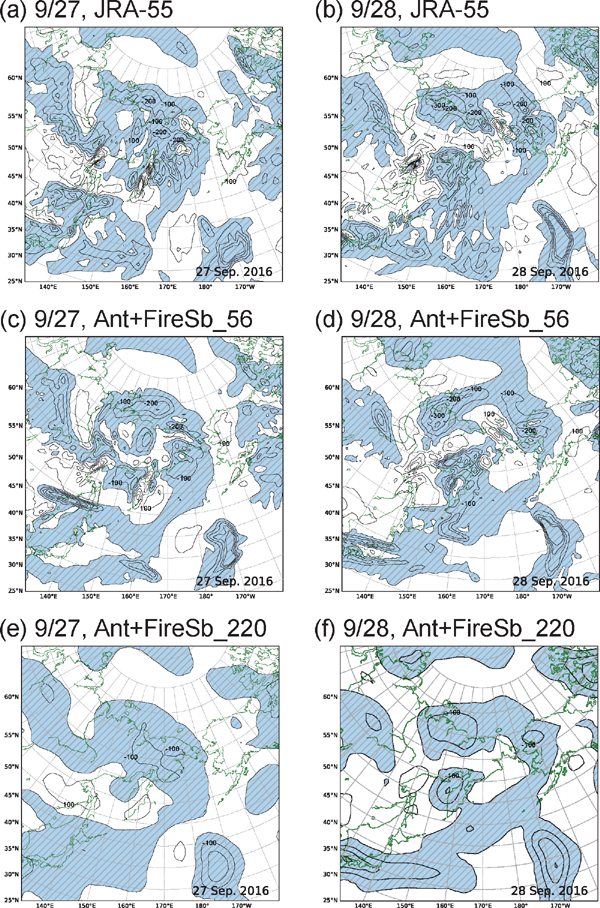
The vertical p-velocity at 700-hPa level (contour interval, 100 hPa d⁻¹) for the (a, b) JRA-55, (a, b) Ant+ Fire_56, and (e, f) Ant+Fire_220. Upper panels, 9/27; lower panels, 9/28. Hatches indicate negative values.

These results suggest that the developed low-pressure system with a large horizontal scale is related to the vertical movement of the BC to the middle and upper troposphere, and the coarse horizontal resolution (∼ 220 km) model is not enough to resolve such vertical movement around the surface low's center and the front line.

4.2 Composite of the developed low events

a. Analytical method

In order to evaluate the generality of the resolution dependency derived from the low-pressure system event in late September 2016, we analyzed the transport process for a similar type of low-pressure system event that occurred in September 2015–2018. Such a low-pressure system requires a large horizontal scale (∼ 2000 km) with a well-developed central pressure located in the “window area” from East Asia/Siberia to the Arctic, that is, it requires the following conditions: (1) a closed cyclone condition, in which the surrounding eight grid points have a higher value in the daily mean SLP over the area within 120–180°E and 50–75°N; (2) a large horizontal scale, in which the zonal/meridional slope within 10° from a central point is blunter relative to the slope at 10°; and (3) the smallest SLP point within 20° is defined as the representative point of the low-pressure system. To avoid false detection around the edge of the area, detection was performed for the area within 110–190°E and 45–80°N. To avoid false detection of the weak low-pressure system, a central pressure > 1000 hPa was discarded. We detected 101 events of the well-developed large low-pressure system from Ant+Fire_56 that took place in September 2015–2018. Since the locations of the low's center were different for these events, the composite mean was calculated for the longitude–latitude grids centered on each low's center of the 101 low-pressure systems. The same 101 low-pressure systems were used for the composite analysis of Ant+Fire_220 to ensure that the same locations of low-pressure systems were used for the transport analysis for both the 56-km and 220-km resolutions. Note that 73 events were detected from Ant+Fire_220 using the same definition as Ant+Fire_56, and the main conclusions of this study do not change when the 73 events are used for analysis instead of the 101 events.

b. Results of the composite analysis

Figure 11 shows the composite of the BC concentrations for the longitude range of ±60° and the latitude range of ±30° from the low's center. There is a clear difference in the surface BC concentrations between the eastward and westward directions from the low's center, with the former being twice as large as the latter (Figs. 11a, f). The high concentration eastward of the low's center is extended southward, implying the south-to-north movement in front of the well-developed low-pressure system as discussed in Section 4.1b. A similar structure of the eastward and westward difference is shown from the surface to the 400-hPa level.

Fig. 11.

Longitude–latitude section centered on the low centers for the composite of the BC concentrations (shading, ng m⁻³) for (a) surface, (b) 850 hPa, (c) 700 hPa, (d) 500 hPa, and (e) 400 hPa of Ant+Fire_56. Black lines indicate SLP (thin, every 4 hPa; thick, every 20 hPa). (f–j) The same as (a–e), but for Ant+Fire_220.

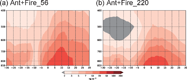
Above 700-hPa levels, the BC concentration of Ant+Fire_56 is larger in magnitude eastward of the low's center than that of Ant+Fire_220. The concentration at (x, y) = (10°, 0°) for Ant+Fire_56 and Ant+Fire_220 is > 20 ng m⁻³ and > 10 ng m⁻³ at 700 hPa, > 7 ng m⁻³ and ∼ 5 ng m⁻³ at 500 hPa, and > 5 ng m⁻³ and > 3 ng m⁻³ at 400 hPa, respectively (Fig. 12). It is noteworthy that the high-BC area above the 500-hPa levels is extended to the north of the low's center for Ant+Fire_56 (Fig. 11), increasing the efficiency of BC transport to the northern area. Table 4 presents the longitudinal mean poleward BC flux at 66°N for the 150°E–160°W (the same longitude range to region 4) for the vertical levels at 850, 775, 700, 600, 500, and 400 hPa of Ant+Fire_56 and Ant+Fire_220, composited for the days of 101 low-pressure systems. The magnitude of the poleward BC flux for the developed low events is about twice as large as that for the September mean. This implies that the BC transport to the Arctic is possibly enhanced by the developed low events, although the September mean flux includes the flux for the developed low events. The magnitude of the poleward BC flux of Ant+Fire_56 is larger than that of Ant+Fire_220, indicating the enhancement of the transport in 56-km simulations. Note that the BC concentration around the low-pressure system is mainly from anthropogenic sources (Fig. 14).

Fig. 12.

The same as Fig. 11, but for the longitude–height section at the latitude = 0° line for the BC concentrations for (a) Ant+Fire_56 and (b) Ant+Fire_220.

Fig. 13.

The same as Fig. 11, but for the vertical p-velocity at 700-hPa level (contour interval, 40 hPa d⁻¹) for (a) Ant+Fire_56 and (b) Ant+Fire_220. Hatches indicate negative values.

Fig. 14.

The same as Fig. 12, but for the anthropogenic BC concentrations.

The analysis of HIPPO data by Wang et al. (2014) indicated ∼ 1–10 ng m⁻³ STP in the Arctic middle troposphere and Schwarz et al. (2017) also indicated the order of ∼ 1–10 ng m⁻³ STP. The September mean BC concentration in the Arctic (> 70°N) middle troposphere (4000–6000 m) around 180°E is about < 4 ng m⁻³ STP for HIPPO data, about < 10 ng m⁻³ STP for Ant+FireSb_56, and about < 8 ng m⁻³ STP for Ant+FireSb_220 (for September 2016), in agreement with their results. Note that the model bias of the fine resolution (56 km) is larger than the coarse resolution (220 km). The BC concentration associated with the low-pressure system is enhanced in 56-km simulations relative to the 220-km simulations (Fig. 12). The implication of the resolution dependency is that the BC transport to the Arctic is enhanced by the reproduction of detailed transport process in higher resolution.

Figure 13 shows the vertical p-velocity at 700 hPa, indicating the ascending motion over the low's center and northward/eastward area. There is a clear difference in magnitude of the ascending motion between Ant+Fire_56 and Ant+Fire_220, and the absolute value in magnitude of Ant+Fire_56 is > 3 times as large as that in Ant+Fire_220. These results are consistent with the event analysis described in Section 4.1b, indicating the generality of the relationship between the ascending motion and the BC concentration in upper levels due to the transport difference between the coarse- (∼ 220 km) and fine- (∼ 56 km) resolution models.

5. Conclusions

The resolution dependency of the transport process of BC from Siberia to the Arctic (from the Siberian forest fire and anthropogenic emissions) related to the developed low-pressure system in September was simulated by the fine- horizontal (56 km) and coarse horizontal (220 km) resolution models of NICAM-SPRINTARS. Each model reproduced the mean surface BC concentration along R/V Mirai's track for a high-BC event on September 25–26, 2016, in the Bering Sea, which originated from the Siberian forest fire. These models also reproduced the mean surface BC concentration at the observation site of Fukue Island in September 2016, which was located downstream of the significant source region in East Asia.

The simulations with the Siberian forest fire emissions showed that the column BC amount around Siberia rapidly declined en route from Siberia to the Bering Sea, reaching a comparable mean concentration in the Bering Sea between the two horizontal resolutions.

The high-BC event in the Bering Sea observed by R/V Mirai occurred simultaneously with the most developed low-pressure system in recent years, which reached the polar region (> 60°N) through a “window area”. When investigating the transport process of this low-pressure system, in the 56-km experiments, the high-BC area in the Bering Sea moved to the Arctic with a filamental structure from the low's center to behind the cold front and ahead of the warm front on September 27–28, 2016. This was accompanied by the ascending and south-to-north movement eastward/northward of the low's center. In contrast, the 220-km experiments produced a widespread high-BC area with a relatively lower maximum concentration, especially in the middle to upper troposphere, associated with the weak ascending motion around the low-pressure system. These results suggest that the 56-km resolution was required to reproduce the inflow of BC to the Arctic due to the high-resolution transport process of the developed low-pressure system around the “window area”.

The composite analysis for the developed low-pressure events in September from 2015–2018 indicated that the high-BC area was located eastward of the low's center, with the ascending motion over the low's center and northward/eastward of the center. The magnitude of the poleward BC flux for the developed low events is about twice as large as that for the September mean. In contrast, the 220-km experiments produced a small magnitude of the high-BC area in the middle to upper troposphere due to the weak ascending motion, indicating the small effect of the BC transport to the Arctic. The results imply that the BC transport to the Arctic by the well-developed low-pressure systems is enhanced in the fine horizontal resolution (∼ 56 km) models relative to the coarse horizontal resolution (∼ 220 km) models. This finding suggests that the coarse horizontal resolution is not adequate to examine the BC transport to the Arctic due to the insufficient resolution of the motions around well-developed low-pressure systems in addition to the insufficient resolution of the wet deposition process suggested by Sato et al. (2016). This implies that the fine horizontal resolution (∼ 56 km) will be desirable for the precise treatment of transport processes in the future chemistry transport models.

Acknowledgments

The authors thank anonymous reviewers for their helpful comments and Dr. K. Ikeda of NIES for his helpful discussion. We also thank the crew of R/V Mirai and the staff at the Global Ocean Development, Inc., and Marine Works Japan, Ltd., for their support with observations throughout the cruise. This work was supported by the FLAGSHIP2020 within priority study 4 (Advancement of meteorological and global environmental predictions utilizing observational “Big Data”) and Program for Promoting Researches on the Supercomputer Fugaku (Large Ensemble Atmospheric and Environmental Prediction for Disaster Prevention and Mitigation) (JPMXP1020351142) of the Ministry of Education, Culture, Sports, Science and Technology (MEXT), and partially supported by the Arctic Challenge for Sustainability Project of MEXT and by JSPS KAKENHI (JP20K12155). The NICAM calculation was performed using the K computer at the RIKEN Center for Computational Science through the HPCI System Research project (Project ID: hp160231, hp170232, hp180181, hp190151). Python matplotlib library was used to draw the figures.

Data Availability Statement

The data analysis files are available in J-STAGE Data. https://doi.org/10.34474/data.jmsj.13384538

• 1) The model outputs of the Nonhydrostatic Icosahedral Atmospheric Model–Spectral Radiation Transport Model for Aerosol Species (NICAM-SPRINTARS)

References

•  Ackerman,  A. S.,  O. B.  Toon,  D. E.  Stevens,  A. J.  Heymsfield,  V.  Ramanathan, and  E. J.  Welton, 2000: Reduction of tropical cloudiness by soot. Science, 288, 1042-1047.
•  Adler,  R.,  J.-J.  Wang,  M.  Sapiano,  G.  Huffman,  D.  Bolvin,  E.  Nelkin, and NOAA CDR Program, 2017: Global Precipitation Climatology Project (GPCP) Climate Data Record (CDR), Version 1.3 (Daily) precipitation. National Centers for Environmental Information, doi:10.7289/V5RX998Z. [Available at https://www.ncei.noaa.gov/access/metadata/landing-page/bin/iso?id=gov.noaa.ncdc:C00999.]
•  Blackmon,  M. L.,  J. M.  Wallace,  N.-C.  Lau, and  S. L.  Mullen, 1977: An observational study of the Northern Hemisphere wintertime circulation. J. Atmos. Sci., 34, 1040-1053.
•  Chikira,  M., and  M.  Sugiyama, 2010: A cumulus parameterization with state-dependent entrainment rate. Part I: Description and sensitivity to temperature and humidity profiles. J. Atmos. Sci., 67, 2171-2193.
•  Dai,  T.,  D.  Goto,  N. A. J.  Schutgens,  X.  Dong,  G.  Shi, and  T.  Nakajima, 2014: Simulated aerosol key optical properties over global scale using an aerosol transport model coupled with a new type of dynamic core. Atmos. Environ., 82, 71-82.
•  Di Pierro,  M.,  L.  Jaeglé, and  T. L.  Anderson, 2011: Satellite observations of aerosol transport from East Asia to the Arctic: Three case studies. Atmos. Chem. Phys., 11, 2225-2243.
•  Goto,  D., 2014: Modeling of black carbon in Asia using a global-to-regional seamless aerosol-transport model. Environ. Pollut., 195, 330-335.
•  Goto,  D.,  T.  Nakajima,  T.  Takemura, and  K.  Sudo, 2011: A study of uncertainties in the sulfate distribution and its radiative forcing associated with sulfur chemistry in a global aerosol model. Atmos. Chem. Phys., 11, 10889-10910.
•  Goto,  D.,  T.  Dai,  M.  Satoh,  H.  Tomita,  J.  Uchida,  S.  Misawa,  T.  Inoue,  H.  Tsuruta,  K.  Ueda,  C. F. S.  Ng,  A.  Takami,  N.  Sugimoto,  A.  Shimizu,  T.  Ohara, and  T.  Nakajima, 2015: Application of a global nonhydrostatic model with a stretched-grid system to regional aerosol simulations around Japan. Geosci. Model Dev., 8, 235-259.
•  Huffman,  G. J.,  R. F.  Adler,  M. M.  Morrissey,  D. T.  Bolvin,  S.  Curtis,  R.  Joyce,  B.  McGavock, and  J.  Susskind, 2001: Global precipitation at one-degree daily resolution from multisatellite observations. J. Hydrometeor., 2, 36-50.
•  Ikeda,  K.,  H.  Tanimoto,  T.  Sugita,  H.  Akiyoshi,  Y.  Kanaya,  C.  Zhu, and  F.  Taketani, 2017: Tagged tracer simulations of black carbon in the Arctic: Transport, source contributions, and budget. Atmos. Chem. Phys., 17, 10515-10533.
• IPCC, 2013: Climate Change 2013: The Physical Science Basis. Contribution of Working Group I to the Fifth Assessment Report of the Intergovernmental Panel on Climate Change.  Stocker,  T. F.,  D.  Qin,  G.-K.  Plattner,  M.  Tignor,  S. K.  Allen,  J.  Boschung,  A.  Nauels,  Y.  Xia,  V.  Bex, and  P. M.  Midgley (eds.), Cambridge University Press, Cambridge, UK and New York, USA, 1535 pp.
•  Ishijima,  K.,  M.  Takigawa,  Y.  Yamashita,  H.  Yashiro,  C.  Kodama,  M.  Satoh,  K.  Tsuboi,  H.  Matsueda,  Y.  Niwa, and  S.  Hirao, 2018: Analysis of high radon-222 concentration events using multi-horizontal-resolution NICAM simulations. SOLA, 14, 111-115.
•  Janssens-Maenhout,  G.,  M.  Crippa,  D.  Guizzardi,  F.  Dentener,  M.  Muntean,  G.  Pouliot,  T.  Keating,  Q.  Zhang,  J.  Kurokawa,  R.  Wankmüller,  H.  Denier van der Gon,  J. J. P.  Kuenen,  Z.  Klimont,  G.  Frost,  S.  Darras,  B.  Koffi, and  M.  Li, 2015: HTAP_v2.2: A mosaic of regional and global emission grid maps for 2008 and 2010 to study hemispheric transport of air pollution. Atmos. Chem. Phys., 15, 11411-11432.
•  Kanaya,  Y.,  F.  Taketani,  Y.  Komazaki,  X.  Liu,  Y.  Kondo,  L. K.  Sahu,  H.  Irie, and  H.  Takashima, 2013: Comparison of black carbon mass concentrations observed by multi-angle absorption photometer (MAAP) and continuous soot-monitoring system (COSMOS) on Fukue Island and in Tokyo, Japan. Aerosol Sci. Technol., 47, 1-10.
•  Kanaya,  Y.,  X.  Pan,  T.  Miyakawa,  Y.  Komazaki,  F.  Taketani,  I.  Uno, and  Y.  Kondo, 2016: Long-term observations of black carbon mass concentrations at Fukue Island, western Japan, during 2009-2015: Constraining wet removal rates and emission strengths from East Asia. Atmos. Chem. Phys., 16, 10689-10705.
•  Kobayashi,  S.,  Y.  Ota,  Y.  Harada,  A.  Ebita,  M.  Moriya,  H.  Onoda,  K.  Onogi,  H.  Kamahori,  C.  Kobayashi,  H.  Endo,  K.  Miyaoka, and  K.  Takahashi, 2015: The JRA-55 reanalysis: General specifications and basic characteristics. J. Meteor. Soc. Japan, 93, 5-48.
•  Lee,  Y. H.,  J.-F.  Lamarque,  M. G.  Flanner,  C.  Jiao,  D. T.  Shindell,  T.  Berntsen,  M. M.  Bisiaux,  J.  Cao,  W. J.  Collins,  M.  Curran,  R.  Edwards,  G.  Faluvegi,  S.  Ghan,  L. W.  Horowitz,  J. R.  McConnell,  J.  Ming,  G.  Myhre,  T.  Nagashima,  V.  Naik,  S. T.  Rumbold,  R. B.  Skeie,  K.  Sudo,  T.  Takemura,  F.  Thevenon,  B.  Xu, and  J.-H.  Yoon, 2013: Evaluation of preindustrial to present-day black carbon and its albedo forcing from atmospheric chemistry and climate model intercomparison project (ACCMIP). Atmos. Chem. Phys., 13, 2607-2634.
•  Mahmood,  R.,  K.  von Salzen,  M.  Flanner,  M.  Sand,  J.  Langner,  H.  Wang, and  L.  Huang, 2016: Seasonality of global and Arctic black carbon processes in the Arctic monitoring and assessment programme models. J. Geophys. Res.: Atmos., 121, 7100-7116.
•  Matsui,  H.,  Y.  Kondo,  N.  Moteki,  N.  Takegawa,  L. K.  Sahu,  Y.  Zhao,  H. E.  Fuelberg,  W. R.  Sessions,  G.  Diskin,  D. R.  Blake,  A.  Wisthaler, and  M.  Koike, 2011: Seasonal variation of the transport of black carbon aerosol from the Asian continent to the Arctic during the ARCTAS aircraft campaign. J. Geophys. Res., 116, D05202, doi:10.1029/2010JD015067.
•  Miyakawa,  T.,  Y.  Kanaya,  Y.  Komazaki,  F.  Taketani,  X.  Pan,  M.  Irwin, and  J.  Symonds, 2016: Intercomparison between a single particle soot photometer and evolved gas analysis in an industrial area in Japan: Implications for the consistency of soot aerosol mass concentration measurements. Atmos. Environ., 127, 14-21.
•  Miyakawa,  T.,  Y.  Komazaki,  C.  Zhu,  F.  Taketani,  X.  Pan,  Z.  Wang, and  Y.  Kanaya, 2019: Characterization of carbonaceous aerosols in Asian outflow in the spring of 2015: Importance of non-fossil fuel sources. Atmos. Environ., 214, 116858, doi:10.1016/j.atmosenv.2019.116858.
•  Miyakawa,  T.,  P.  Mordovskoi, and  Y.  Kanaya, 2020: Evaluation of black carbon mass concentrations using a miniaturized aethalometer: Intercomparison with a continuous soot monitoring system (COSMOS) and a single-particle soot photometer (SP2). Aerosol Sci. Technol., 54, 811-825.
•  Myhre,  G.,  N.  Bellouin,  T. F.  Berglen,  T. K.  Berntsen,  O.  Boucher,  A.  Grini,  I. S. A.  Isaksen,  M.  Johnsrud,  M. I.  Mishchenko,  F.  Stordal, and  D.  Tanré, 2007: Comparison of the radiative properties and direct radiative effect of aerosols from a global aerosol model and remote sensing data over ocean. Tellus B, 59, 115-129.
•  Myhre,  G.,  B. H.  Samset,  M.  Schulz,  Y.  Balkanski,  S.  Bauer,  T. K.  Berntsen,  H.  Bian,  N.  Bellouin,  M.  Chin,  T.  Diehl,  R. C.  Easter,  J.  Feichter,  S. J.  Ghan,  D.  Hauglustaine,  T.  Iversen,  S.  Kinne,  A.  Kirkevåg,  J.-F.  Lamarque,  G.  Lin,  X.  Liu,  M. T.  Lund,  G.  Luo,  X.  Ma,  T.  van Noije,  J. E.  Penner,  P. J.  Rasch,  A.  Ruiz,  Ø.  Seland,  R. B.  Skeie,  P.  Stier,  T.  Takemura,  K.  Tsigaridis,  P.  Wang,  Z.  Wang,  L.  Xu,  H.  Yu,  F.  Yu,  J.-H.  Yoon,  K.  Zhang,  H.  Zhang, and  C.  Zhou, 2013: Radiative forcing of the direct aerosol effect from AeroCom Phase II simulations. Atmos. Chem. Phys., 13, 1853-1877.
•  Samset,  B. H.,  G.  Myhre,  M.  Schulz,  Y.  Balkanski,  S.  Bauer,  T. K.  Berntsen,  H.  Bian,  N.  Bellouin,  T.  Diehl,  R. C.  Easter,  S. J.  Ghan,  T.  Iversen,  S.  Kinne,  A.  Kirkevåg,  J.-F.  Lamarque,  G.  Lin,  X.  Liu,  J. E.  Penner,  Ø.  Seland,  R. B.  Skeie,  P.  Stier,  T.  Takemura,  K.  Tsigaridis, and  K.  Zhang, 2013: Black carbon vertical profiles strongly affect its radiative forcing uncertainty. Atmos. Chem. Phys., 13, 2423-2434.
•  Sand,  M.,  T. K.  Berntsen,  K.  von Salzen,  M. G.  Flanner,  J.  Langner, and  D. G.  Victor, 2016: Response of Arctic temperature to changes in emissions of short-lived climate forcers. Nat. Climate Change, 6, 286-289.
•  Sato,  Y.,  H.  Miura,  H.  Yashiro,  D.  Goto,  T.  Takemura,  H.  Tomita, and  T.  Nakajima, 2016: Unrealistically pristine air in the Arctic produced by current global scale models. Sci. Rep., 6, 26561, doi:10.1038/srep26561.
•  Satoh,  M.,  T.  Matsuno,  H.  Tomita,  H.  Miura,  T.  Nasuno, and  S.  Iga, 2008: Nonhydrostatic icosahedral atmospheric model (NICAM) for global cloud resolving simulations. J. Comput. Phys., 227, 3486-3514.
•  Satoh,  M.,  H.  Tomita,  H.  Yashiro,  H.  Miura,  C.  Kodama,  T.  Seiki,  A. T.  Noda,  Y.  Yamada,  D.  Goto,  M.  Sawada,  T.  Miyoshi,  Y.  Niwa,  M.  Hara,  T.  Ohno,  S.  Iga,  T.  Arakawa,  T.  Inoue, and  H.  Kubokawa, 2014: The nonhydrostatic icosahedral atmospheric model: Description and development. Prog. Earth Planet. Sci., 1, 18, doi:10.1186/s40645-014-0018-1.
•  Schwarz,  J. P.,  B.  Weinzierl,  B. H.  Samset,  M.  Dollner,  K.  Heimerl,  M. Z.  Markovic,  A. E.  Perring, and  L.  Ziemba, 2017: Aircraft measurements of black carbon vertical profiles show upper tropospheric variability and stability. Geophys. Res. Lett., 44, 1132-1140.
•  Serreze,  M. C.,  A. H.  Lynch, and  M. P.  Clark, 2001: The Arctic frontal zone as seen in the NCEP-NCAR reanalysis. J. Climate, 14, 1550-1567.
•  Spackman,  J. R.,  R. S.  Gao,  W. D.  Neff,  J. P.  Schwarz,  L. A.  Watts,  D. W.  Fahey,  J. S.  Holloway,  T. B.  Ryerson,  J.  Peischl, and  C. A.  Brock, 2010: Aircraft observations of enhancement and depletion of black carbon mass in the springtime Arctic. Atmos. Chem. Phys., 10, 9667-9680.
•  Stohl,  A., 2006: Characteristics of atmospheric transport into the Arctic troposphere. J. Geophys. Res., 111, D11306, doi:10.1029/2005JD006888.
•  Suzuki,  K.,  T.  Nakajima,  M.  Satoh,  H.  Tomita,  T.  Takemura,  T. Y.  Nakajima, and  G. L.  Stephens, 2008: Global cloud-system-resolving simulation of aerosol effect on warm clouds. Geophys. Res. Lett., 35, L19817, doi:10.1029/2008GL035449.
•  Takata,  K.,  S.  Emori, and  T.  Watanabe, 2003: Development of the minimal advanced treatments of surface interaction and runoff. Global Planet. Change, 38, 209-222.
•  Takemura,  T.,  H.  Okamoto,  Y.  Maruyama,  A.  Numaguti,  A.  Higurashi, and  T.  Nakajima, 2000: Global threedimensional simulation of aerosol optical thickness distribution of various origins. J. Geophys. Res., 105, 17853-17873.
•  Takemura,  T.,  T.  Nakajima,  O.  Dubovik,  B. N.  Holben, and  S.  Kinne, 2002: Single-scattering albedo and radiative forcing of various aerosol species with a global three-dimensional model. J. Climate, 15, 333-352.
•  Takemura,  T.,  M.  Egashira,  K.  Matsuzawa,  H.  Ichijo,  R.  O'Ishi, and  A.  Abe-Ouchi, 2009: A simulation of the global distribution and radiative forcing of soil dust aerosols at the Last Glacial Maximum. Atmos. Chem. Phys., 9, 3061-3073.
•  Taketani,  F.,  T.  Miyakawa,  H.  Takashima,  Y.  Komazaki,  X.  Pan,  Y.  Kanaya, and  J.  Inoue, 2016: Shipborne observations of atmospheric black carbon aerosol particles over the Arctic Ocean, Bering Sea, and North Pacific Ocean during September 2014. J. Geophys. Res.: Atmos., 121, 1914-1921.
•  Tomita,  H., and  M.  Satoh, 2004: A new dynamical framework of nonhydrostatic global model using the icosahedral grid. Fluid Dyn. Res., 34, 357-400.
•  Quinn,  P. K.,  T. S.  Bates,  E.  Baum,  N.  Doubleday,  A. M.  Fiore,  M.  Flanner,  A.  Fridlind,  T. J.  Garrett,  D.  Koch,  S.  Menon,  D.  Shindell,  A.  Stohl, and  S. G.  Warren, 2008: Short-lived pollutants in the Arctic: Their climate impact and possible mitigation strategies. Atmos. Chem. Phys., 8, 1723-1735.
•  Veira,  A.,  S.  Kloster,  N. A. J.  Schutgens, and  J. W.  Kaiser, 2015: Fire emission heights in the climate system-Part 2: Impact on transport, black carbon concentrations and radiation. Atmos. Chem. Phys., 15, 7173-7193.
•  Wang,  Q.,  D. J.  Jacob,  J. R.  Spackman,  A. E.  Perring,  J. P.  Schwarz,  N.  Moteki,  E. A.  Marais,  C.  Ge,  J.  Wang, and  S. R. H.  Barrett, 2014: Global budget and radiative forcing of black carbon aerosol: Constraints from pole-to-pole (HIPPO) observations across the Pacific. J. Geophys. Res.: Atmos., 119, 195-206.