Review Articles
Hansch-藤田解析の原点からの新たな定量的構造活性相関解析法の構築
2013 年 38 巻 2 号 p. 60-67

詳細
2013 年 38 巻 2 号 p. 60-67
The advent of QSAR began with the encounter of Professors Corwin Hansch and Toshio Fujita in June 1961, as described by themselves.1,2) More than half a century has passed since their discovery of a general approach to the formulation of QSAR. Since its conception, this approach has provided a new perspective for chemical-biological interactions as well as a number of successes in drug discovery. Now it is time to develop a new and promising approach based on their QSAR with the aid of modern, powerful molecular calculations on a whole ligand–protein complex structure while staying true to the original ideas of Hansch and Fujita as much as possible. Their seminal ideas are succinctly and clearly expressed in their early publications.3–5) With respect to their key concepts, which focused on (1) linear free-energy principle (LFEP)6) and additivity/decomposition of free-energy change and (2) LFEP parameters represented by Hammett σ, we now will discuss two topics relating to (1) and (2) by comparing results and implications obtained using the original and our QSAR approaches.
A few remarks concerning the Hansch–Fujita equation may be appropriate. A general form of the Hansch–Fujita equation is expressed by Eq. (1):
 | (1) |
where C is a concentration having a standard response in a standard time. σ and log P are the Hammett constant and partition coefficient (to be more precise, logarithm of the partition coefficient P between 1-octanol and water), respectively. When C can be assumed to correspond to the equilibrium constant, log(1/C) is proportional to the free-energy change (log(1/C)=−ΔG/(2.303RT)) of the overall process from administration of a drug to interaction with a target receptor. Hence, Eq. (1) states that the overall free-energy change for a congeneric series of ligands is expressible as the sum of representative energy terms, each of which follows LFEP.
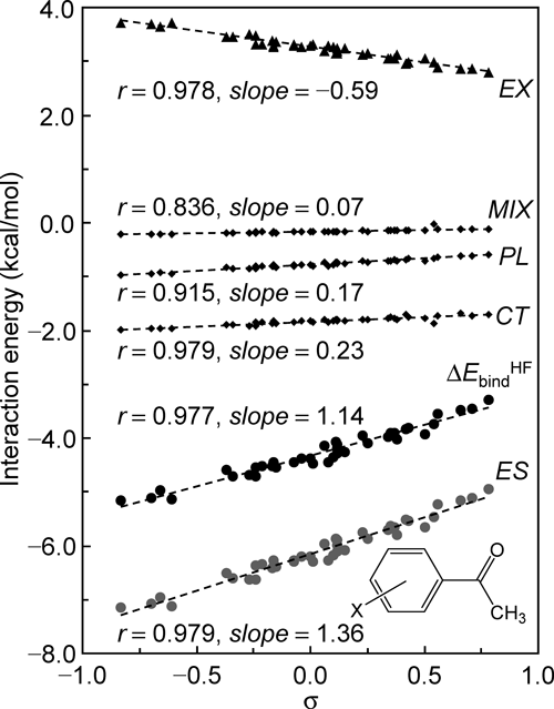
2. Reassessment of parameters used in traditional QSAR, using molecular calculations 2.1. Hammett σThe Hammett σ constant has long been known as one of the most important LFEP parameters that correlate with biological activity. It is a conventionally used electronic parameter in studies of enzymatic QSAR. However, it is not necessarily obvious why σ represents variations in the free-energy change associated with the complex formation between a congeneric series of ligands and their target protein. We comprehensively reevaluate experimentally derived parameter σ, confirming that it represents intermolecular interaction energy terms, by applying a molecular orbital (MO) calculation (Hartree–Fock (HF)/6-31G(d,p)) to a simple ligand–protein complex model, complexes of a series of para and meta mono-substituted acetophenones with N′-methylacetamide.7) Figure 1 shows that the total binding energy (ΔEHFbind) is nicely linear with σ. Variations of energy components obtained with the energy decomposition analysis developed by Kitaura and Morokuma8) are also plotted in Fig. 1, revealing that all the energy components are linear with σ and that the electrostatic component (ES) governs ΔEHFbind. Similarly, the hydration (ΔGsol) and dispersion (Edisp) energy changes accompanying the complex formation are nicely linear with σ (r=0.967, slope=−0.855 (conductor-like polarizable continuum model (CPCM)9)/HF/6-31G(d,p)) and r=0.973, slope=1.19 (MP210)/6-31G(d,p)), respectively). It is noteworthy that ΔGsol shows a nearly perfect correlation with ΔEHFbind (r=0.995, slope=−0.693). These results suggest that the intermolecular energy terms obtained through MO calculations for full complex structures of a congeneric series of ligands with a protein basically follow LFEP, as represented by Hammett σ, and can bridge the gap between the traditional Hansch–Fujita and modern QSAR approaches.
The partition coefficient log Psol (Psol=Csol/Cwater) can be expressed with the Gibbs free-energy, enthalpy, and entropy differences.
 | (2) |
Starting from the basic relation Eq. (2), we formulated a semiempirical correlation Eq. (3) for log Psol (sol=chloroform (CL) and 1-octanol (oct))11–13):
 | (3) |
where ΔEsol (calculated with CPCM/HF/6-31+G(d)//HF/3-21G*) is the solvation energy difference between aqueous and organic solvent phases, and ASA is the accessible surface area of solute molecules. IHAc and Isol are indicator variables. IHAc takes unity for hydrogen-bonding acceptors but otherwise zero, and Isol takes unity for log PCL and zero for log Poct. Although IHAc and Isol were introduced empirically, physicochemical meanings of these indicator variables were discussed adequately in the original paper.12) Equation (3) can give an excellent prediction of log Psol for non-hydrogen bonders and hydrogen-bonding acceptors (r=0.972, s=0.283 for training compounds (n=208) and r=0.973, s=0.296 for external test ones (n=51)). When deriving Eq. (3) from Eq. (2), we assumed that (1) ΔEsol on the right-hand side of Eq. (3) corresponds to ΔHsol in Eq. (2) (note that ΔH≈ΔE in solution) and that (2) ASA, IHAc, and Isol effectively express ΔSsol. In fact, the coefficient of ΔEsol in Eq. (3) takes a value (a=−0.776) close to the expected one (−1/(2.303RT)=−0.734 at 298 K). However, for hydrogen-bonding donors, that is approximately half of the expected value (∼0.34). This result probably suggests the deficiency in continuum solvation models (i.e., assumption of uniform distribution) used in PCM,9) generalized Born (GB),14) and Poisson–Boltzmann (PB)14) types of calculations. Figure 2 shows observed and calculated log PCL values (chloroform/water) of simple molecules, together with calculated ones with reference interaction site model (RISM),15,16) which explicitly considers the (non-uniform) distribution of solvent molecules. The standard error of log PCL calculated with RISM (0.670) is, however, considerably larger than that with CPCM (0.296).
At present, it is difficult to reproduce log Psol within chemical accuracy (∼0.5 kcal/mol) only by means of theoretical calculations such as the ab initio self-consistent reaction field (SCRF) type of MOs and RISM. It should be very important to make the status of the current solvation models higher in predicting the solvation energy by extending and elaborating the current models.

We previously proposed a novel QSAR procedure called linear expression by representative energy terms (LERE)-QSAR17–21) involving molecular calculations such as an ab initio fragment molecular orbital (FMO) one.22) The idea of LERE-QSAR follows that of the Hansch–Fujita type of QSAR. The first assumption made in formulating the LERE-QSAR equation is that the free-energy terms comprising the overall free-energy change associated with complex formation are all additive.
 | (4) |
ΔGobs on the left-hand side is the overall free-energy change calculated from the observed inhibitory potency (ΔGobs=RT ln C, where C is the same in Eq. (1)). ΔGbind and ΔGsol (typically taken as dominant free-energy terms) are the intrinsic binding interaction free-energy of an inhibitor with a protein and the solvation free-energy change associated with complex formation, respectively. ΔGothers, the sum of free-energy terms other than representative free-energy terms ΔGbind and ΔGsol, is assumed to be linear with that of representative free-energy terms (LERE approximation). ΔGothers consists of, for instance, the structural deformation (adaptation/induced fitting) energy associated with complex formation
 | (5) |
where ΔGothers is expected to work as a penalty term (β<0 and/or const1>0). The last assumption is the entropy–enthalpy compensation,23) which is expected to effectively hold for the binding of a series of ligands with a protein:
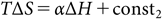 | (6) |
where α>0.

ΔGsol is replaced by the dominant polar (electrostatic) contribution ΔGsolpol because the non-polar contribution is often negligible, and most of ΔGsolpol is considered to come from the enthalpic contribution.19) Combining the above three equations yields the following expression (LERE-QSAR equation):
 | (7) |
The coefficient γ on the right-hand side of the above equation is a constant determined by α and β (γ=(1−α)(1+β)). Representative energy terms other than ΔEbind and ΔGsolpol, such as the dissociation of a ligand (ΔGdiss) and deformation free-energy changes, are added to Eq. (7) if needed. ΔEbind is computable using ab initio MO calculations such as FMO22) and ONIOM,26) and ΔGsolpol is computable with continuum solvation models such as GB,14) PB,14) PCM,9) and RISM.27) Table 1 concisely lists an estimation of representative energy terms and the entropic energy used in the LERE procedure. A general procedure for the LERE-QSAR analysis consists of two steps: (1) determine a complex structure, usually by carrying out classical molecular mechanics and molecular dynamics calculations repeatedly, and (2) calculate ΔX (X=Ebind and Gsolpol) as ΔX=Xcomplex−Xprotein−Xligand (supermolecular approximation).
| Energy | Symbol | Method (program) | Ref. |
|---|---|---|---|
| Binding energy | ΔEbind | Molecular Mechanics (AMBER) | 28 |
| Fraction with Caps (MFCC) | 29 | ||
| FMO (ABINIT-MP and GAMESS) | 22 | ||
| QM/MM (ONIOM) | 26 | ||
| Solvation energy | ΔGsol | GB/PB (AMBER) | 14 |
| PCM (Gaussian and GAMESS) | 9 | ||
| Hybrid (PCM/PB(GB)) | 30 | ||
| RISM | 27 | ||
| Entropic energy | −TΔS | Normal mode calculation | 31, 32 |
| Quasi-harmonic approximation | 33 | ||
| Entropy–enthalpy compensation | 23 |
Although several free-energy calculation methods34) have been proposed such as the thermodynamics integration, free-energy perturbation, Bennett’s acceptance ratio, linear interaction energy (LIE),35) and solvated interaction energy (SIE),36) the purpose of our research is to develop an LFEP-based QSAR that can predict the overall binding free-energy change within chemical accuracy, which is unattainable by approaches other than LERE-QSAR, at least for now.
Substituted benzenesulfonamides (BSAs) and biphenylsulfonamides (BSs), shown in Figs. 4(a) and (b), inhibit bovine carbonic anhydrase II (CA) and matrix metalloproteinase-9 (MMP), respectively.

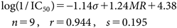
During their complex formation, the anionized sulfonamide (SO2NH−) in BSAs and carboxylate (CO2−) in BSs coordinate to the zinc atom (Zn2+) in the active sites of CA and MMP, respectively. Hansch37) and Verma38) reported QSAR Eqs. (8a) and (8b) for inhibition of CA by BSAs and that of MMP by BSs, respectively:
 | (8a) |
 | (8b) |
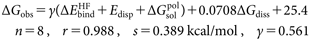
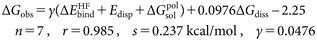
where π in Eq. (8a) is a hydrophobic constant of a substituent (X in Fig. 4(a)), which is defined as log P (substituted benzene)−log P (benzene). MR in Eq. (8b) represents the dispersion interaction of a substituent (X in Fig. 4(b)). It should be noted that signs of coefficient of σ are opposite in Eqs. (8a) and (8b); thus, we focused on the reasons the opposite direction of substituent electronic effect is observed in complex formations CA–BSA and MMP–BS. We performed the LERE-QSAR analysis using the three representative energy terms: ΔEbind (ONIOM (HF-D39)/6-31G : Amber), electronic embedding scheme), ΔGsolpol (GB), and ΔGdiss (integral equation formalism PCM (IEFPCM)40)/B3LYP41)/6-31+G(d,p) and IEFPCM/HF/6-31+G(d) for CA–BSAs18,20) and MMP–BSs,21) respectively) for complexes CA–BSA and MMP–BS and obtained Eqs. (9a) and (9b) with s (standard deviation)<0.3 kcal/mol:
 | (9a) |
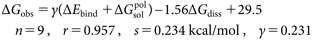 | (9b) |
It is noted that the coefficients (γ) in Eqs. (9a) and (9b) are nearly the same value. Figure 5(a) shows that the relative contribution from ΔGsolpol and ΔGdiss overwhelms that from ΔEbind and that the former governs the overall free-energy change ΔGobs. Conversely, Fig. 5(b) shows that the latter governs ΔGobs. There is an anticorrelation between ΔEbind and ΔGsolpol in Eqs. (9a) and (9b) (r=−0.922 and −0.862, respectively (the negative sign of r indicates a negative slope hereafter)), as frequently observed. As demonstrated in the previous section “Hammett σ,” ΔEbind and ΔGsolpol are expected to show positive and negative correlations with Hammett σ, respectively.
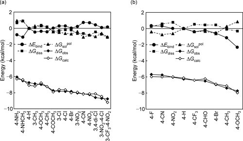
As can be seen in Figs. 6(a) and (b), variations of ΔGsolpol in CA–BSAs and ΔEbind in MMP–BSs are mostly from the zinc atom.
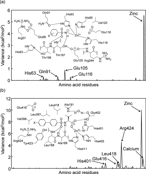
The opposite signs of the coefficients of σ in Eqs. (8a) and (8b) are now clearly explainable from differences in representative energy terms between complex formations CA–BSA and MMP–BS. This instructive case study demonstrates that LERE-QSAR has a considerable advantage over the traditional QSAR, although there is no logical conflict between the two.
2. Comparative LERE-QSAR analysis of inhibitory activity of sialic acid analogues on two neuraminidases17,19)Neuraminidases (NAs) are ubiquitous exoglycohydrolases that hydrolyze the terminal sialic acids of glycoproteins and glycolipids and are widely distributed in nature, from viruses, microorganisms, and fungi to higher animals and humans.42) Among them, influenza virus NAs have been studied extensively as a target for influenza disease, and anti-influenza drugs have been developed. These drugs have the potential to affect the activities of endogenous human NAs.43,44) Thus, it is of great importance to examine differences in the binding mechanism between the influenza virus and human NAs with a series of sialic acid analogues. We selected influenza virus neuraminidase-1 (N1-NA) and human neuraminidase-2 (hNEU2). Amino acid residues important for recognition of sialic acids are basically conserved in N1-NA and hNEU2.19)
Table 2 lists sialic acid analogues, Sets I and II compounds used in the study. We constructed complexes of N1-NA and hNEU2 with Sets I and II compounds, respectively, and then performed the LERE-QSAR analysis using the three representative energy terms: ΔEbind (=ΔEHFbind+Edisp, FMO/MP2/6-31G), ΔGsolpol (hybrid (CPCM/PB)30) and PB for N1-NA–Set I and hNEU2–Set II compounds, respectively), and ΔGdiss (CPCM/HF/6-31+G(d,p)).
;%0A%09%09%09newWindow.document.open();%0A%09%09%09newWindow.document.write('<img src=%22./Graphics/38_D12-082_T02.png%22>');%0A%09%09%09newWindow.document.close();%0A%09%09)
| (a) Set I compound | N1-NA | ||||
|---|---|---|---|---|---|
| No. | Type | R1 (fragment A)a) | R2 (fragment C)a) | IC50b) | ΔGobsc) |
| 1 | I | OH | NH3+ | 6300 | −7.38 |
| 2 | I | OCH2CH2CH3 | NH3+ | 180 | −9.57 |
| 3 | I | OCH(CH3)(CH2CH3)(R) | NH3+ | 10 | −11.35 |
| 4 d) | I | OCH(CH2CH3)2 | NH3+ | 1 | −12.77 |
| 5 | I | OH | NHC(=NH2+)NH2 | 100 | −9.93 |
| 6 | I | OCH2CH2CH3 | NHC(=NH2+)NH2 | 2 | −12.34 |
| 7 | I | OCH(CH3)(CH2CH3)(R) | NHC(=NH2+)NH2 | 0.5 | −13.19 |
| 8 | I | OCH(CH2CH3)2 | NHC(=NH2+)NH2 | 0.5 | −13.19 |
| (b) Set II compound | hNEU2 | ||||
| No. | Type | R1 (fragment A)a) | R2 (fragment C)a) | K i e) | ΔGobsf) |
| 1 | II | OCH2CH(CH3)2 | OH | 0.88 | −4.33 |
| 2 | II | OCH2CH2CH2(OH) | OH | 0.74 | −4.44 |
| 3 | II | OCH2CH(OH)CH2(OH) | OH | 1.4 | −4.05 |
| 4 | II | CH(OH)CH(OH)CH2(OH) | OH | 0.14 | −5.47 |
| 5 g) | II | CH(OH)CH(OH)CH2(OH) | NHC(=NH2+)NH2 | 0.017 | −6.77 |
| 6 h) | III | CH(CH2CH3)2 | NHC(=NH2+)NH2 | 0.33 | −4.94 |
| 7 d) | I | OCH(CH2CH3)2 | NH3+ | 5 | −3.26 |
a) Fragments A and C correspond to R1 and R2, respectively. Fragment B denotes the rest of structure (without fragments A and C). b) Taken from Ref. 45 (In nM). c) ΔGobs=RT ln IC50 (T=310 K). d) Oseltamivir (Tamiflu). e) Taken from Ref. 46 (In mM). f) ΔGobs=RT ln Ki (T=310 K). g) Zanamivir (Relenza). h) Peramivir (Rapiacta).
The observed overall free-energy change ΔGobs for complex formation of N1-NA and hNEU2 with sialic acid analogues is excellently reproducible with the LERE-QSAR Eqs. (10a) and (10b), respectively (s<0.4 kcal/mol).
 | (10a) |
 | (10b) |
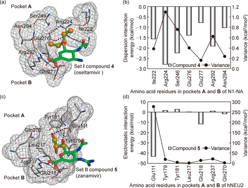
As can be seen in Figs. 7(a) and (b), ΔGdiss varies depending on the types of cationic groups in fragment C (NH3+ and NHC(=NH2+)NH2, shown in Table 2). Figure 7(a) for N1-NA–Set I compounds shows that the electrostatic contribution from two electrostatic energy terms (ΔEHFbind and ΔGsolpol) in Eq. (10a) is considerably smaller than that from the dispersion energy term (Edisp) because of compensation between the two electrostatic energy terms (r=−0.950). Consequently, Edisp governs ΔGobs in complex formation of N1-NA with Set I compounds.17) Conversely, Fig. 7(b) for hNEU2–Set II compounds shows that the contribution of Edisp is considerably smaller than that of the electrostatic energy contribution in Eq. (10b). Hence, ΔEHFbind governs ΔGobs in complex formation of hNEU2 with Set II compounds.19)

It should be noted that remarkable differences in the coefficient (γ) and intercept (corresponds to const3 in Eq. (7)) exist between Eqs. (10a) and (10b). The coefficient (β) and intercept (const1) in Eq. (5) (LERE approximation) are expressed with α, γ, const2, and const3 in Eqs. (6) and (7): (α+γ−1)/(1−α) and (const2+const3)/(1−α), respectively. When assuming α=0.70,25,47–49) β takes 0.87 and −0.84, and const3 is 85+3.3 const2 (relative value: 85 kcal/mol) and −7.5+3.3 const2 (−7.5 kcal/mol) for Eqs. (10a) and (10b), respectively. Using β and const1 in Eq. (5) (LERE approximation/assumption), we will now discuss the effect of ΔGothers on the coefficient and intercept in Eqs. (10a) and (10b). The positive β (0.87) and large const1 (85 kcal/mol) for Eq. (10a) indicate that ΔGothers varies in a parallel manner with the sum of representative energy terms and yields a large positive constant in Eq. (10a) as a penalty energy. In contrast, the negative β (−0.84) and smaller const1 (−7.5 kcal/mol) for Eq. (10b) indicate that ΔGothers nearly cancels out the sum of representative energy terms because of negative correlation with the sum. As expected (β<0 and/or const1>0), ΔGothers is now confirmed to work as the penalty energy both in Eqs. (10a) and (10b) but behaves differently. This is probably due to differences in the primary interaction governing the overall free-energy change, Edisp and ΔEHFbind for N1-NA–Set I and hNEU2–Set II compounds, respectively. Figures 8(a), (b) and (c), (d) show that contributions of Edisp (N1-NA–Set I compounds) and ΔEHFbind (hNEU2–Set II compounds) from amino acid residues located in close proximity to fragment A (shown in Table 2) dominantly determine the overall free-energy change ΔGobs, respectively.
The second case study demonstrates that the LERE-QSAR equation is significantly informative concerning variations of ligand–protein interaction energy.
We feel some concern about QSAR models in which descriptors (explaining variables) are selected “automatically” from a large pool of candidate descriptors, as sometimes found in recent publications. We believe QSAR models should be interpretable physicochemically and informative chemically and biologically, not merely statistically acceptable. It is important to make efforts for constructing a fundamental QSAR that can accurately describe the essence of chemical-biological interactions. As mentioned at the beginning of this paper, the encounter of the two perspicacious scientists has had a strong and lasting influence on later generations.
We would like to express our sincere gratitude to Professor Toshio Fujita (Kyoto University), who has been giving us valuable and warm suggestions during the course of our studies. We also sincerely thank Professor Cynthia Selassie (Pomona College, US) for improving words and Mr. Takuya Sugimoto (University of Tokushima) for preparing a part of figures.