Application of a Bayesian ordinal animal model for the estimation of breeding values for the resistance to Monilinia fruticola (G.Winter) Honey in progenies of peach [Prunus persica (L.) Batsch]

Abstract

Fruit brown rot caused by Monilinia spp. is the most important fungal disease of stone fruits worldwide. Several phenotyping protocols to accurately characterize and evaluate brown rot infection have been proposed; however, the outcomes from those studies have not led to consistent advances in resistance breeding programs. Breeding for disease resistance is one of the most challenging objectives for crop improvement because disease expression is tetrahedral: it is simultaneously influenced by agent, host, environment, and human management. The present study presents a strategy based on Bayesian inference to analyze a peach breeding progeny for resistance to brown rot, evaluated using a polytomous ordinal scale. A pedigree containing two sources of resistance, one from peach and the other from almond, several commercial cultivars, and two segregating populations were analyzed to estimate the narrow-sense heritability (h²) and breeding values (EBVs) for brown rot resistance in progenies. Results show promise for genetic improvement of disease resistance and other traits characterized by strong environmental interactions.

Introduction

Brown rot (BR) is the general term given to the symptoms of infection and sporulation on stone fruit, primarily by Monilinia fructicola (G.Winter) Honey, and to a lesser extent by Monilinia laxa (Aderh. & Ruhland) and Monilinia fructigena Honey. BR is the most important disease of peach worldwide (Gradziel 2003, Ogawa and English 1991) and the frequent application of fungicides required to control it remains a major constraint to sustainable production. Consequently, genetic resistance to BR is highly desirable in new cultivars.

Various resistance and tolerance germplasm sources are known (Byrne et al. 2012), and several efforts have examined the way in which M. fructicola infects fruits (Lee and Bostock 2007, Lee et al. 2010). Although fruit traits associated with resistance (Gradziel 2003) and part of their genetic components (Martínez-García et al. 2013) have been characterized, successful breeding of resistant commercial cultivars remains elusive, due in part to the strong environmental influence, the absence of a focused research effort including the development of an efficient evaluation criteria. Characteristics of the fruit epidermis, such as thickness of the cuticle and epicuticular wax layer, and concentrations of pectin, phenolic, chlorophyll, and other biochemical compounds associated with tissue maturation (Gradziel and Wang 1993, Lee and Bostock 2007), are associated with the degree of resistance within a given phenotype when the fruits are not wounded. Epidermal barriers can be lost following mechanical or insect damage, leaving only mesocarp resistance factors such as high phenolic concentration or flesh textural integrity, which may be commercially undesirable (Gradziel 2003).

Procedures for characterizing epidermal characteristics are labor intensive, expensive, and inconsistent (Byrne et al. 2012). In wounded fruit, where the epidermis has been breached, Martínez-García et al. (2013) identified three putative quantitative trait loci (QTLs) and two candidate genes associated with the BR resistance. However, because the phenotypic data and residuals distribution from non-wounded fruit exhibited serious departures from a normal distribution due to serious departures from homoscedasticity (i.e. heterogeneity of variance), the data was not used for QTL analysis, which assumes homoscedasticity. In this case, data transformation would not help to alleviate the issues while not altering intuitiveness of the phenotypic scale during conclusion drawing. Information generated through artificial inoculation on non-wounded fruit is considered more reliable and representative of BR field resistance (Byrne et al. 2012).

In peaches bred for canning, normally undesirable fruit epidermis-based resistance such as high phenolic concentration and cellular integrity can be targeted, since the epidermis is removed during processing. Towards this goal, sources of epidermis-based resistance from peach, including the resistant cultivar ‘Bolinha’ (Feliciano et al. 1987), as well as from almond and related species have been incorporated into advanced breeding selections, through genetic introgression (Gradziel 2002, Gradziel et al. 2003). While BR resistance has been improved, the derived germplasm often shows reduced quality for important commercial traits as a result of linkage drag (Gradziel 2003, Gradziel and Wang 1993).

Concurrent selection for epidermis-based resistance and good fruit quality is consequently highly desirable, despite the genetic complexity of these traits and their often exotic origins. Towards this goal, a strategy based on Bayesian inference is presented as an application of the individual model (also known as “the animal model” in animal breeding literature), referred to here as the Bayesian ordinal animal model (BOAM). A pedigree-based narrow-sense heritability (h²) was estimated and the estimated breeding values (EBVs) were obtained by fitting ordinal logistic regression by means of the Gibbs sampler integrated in JAGS (Plummer 2003). To evaluate the robustness of BOAM, the evaluation of the goodness-of-fit was performed for several models, using distinct priors for the probability distribution of the square root of the additive genetic variance $\left(\sqrt{{\sigma }_a^2}\right)$. Finally, a series of comparisons were performed. The first set compared the EBVs from each model, their correlations, and the ranking of individuals. Subsequently, a comparison of the ranking of the EBVs obtained from the analysis of a severity index evaluated through restricted maximum likelihood (REML) was performed.

Materials and Methods

Plant material

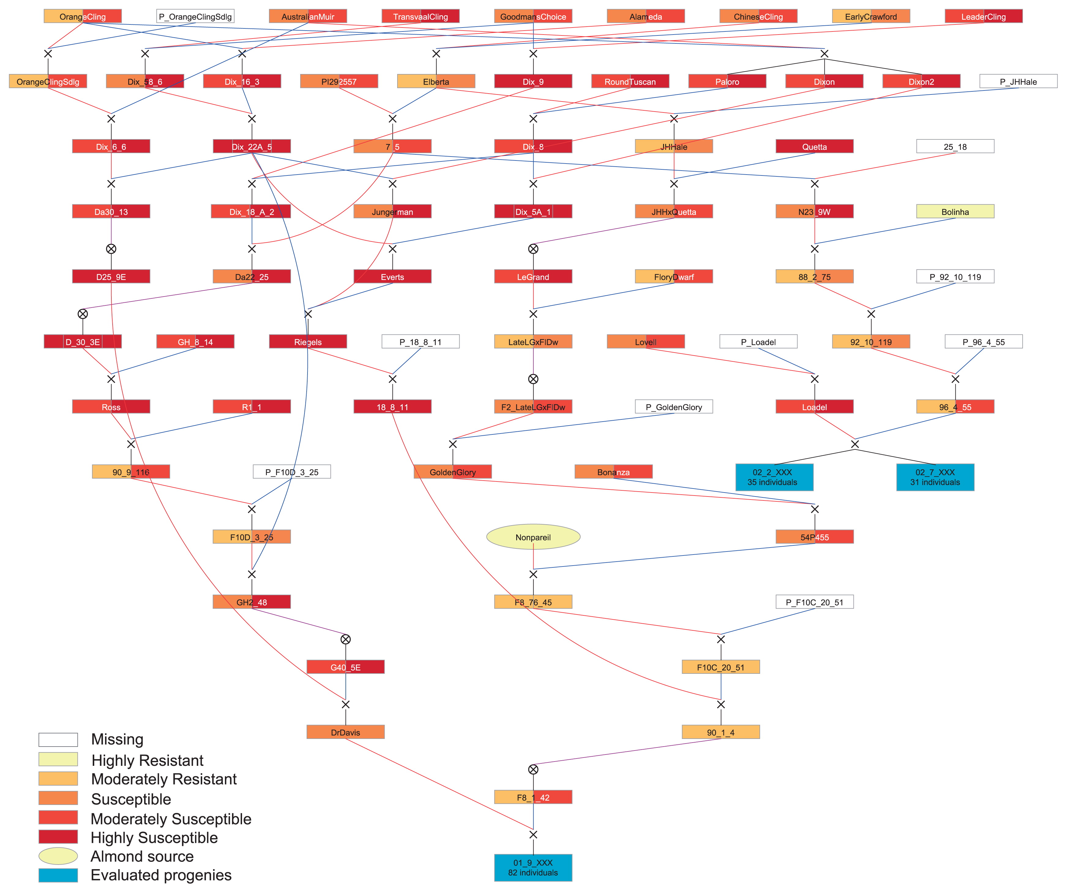
The pedigree analyzed is composed of 221 accessions, including processing peach cultivars and breeding selections, the almond cultivar ‘Nonpareil’, and two segregating mapping populations (PopBR-1 and PopBR-2) resulting from the crosses ‘Dr. Davis’ × ‘F8,1-42’ and ‘Loadel’ × ‘96,4-55’, respectively (Fig. 1). The first cross, involved a resistant modern cultivar and a breeding line possessing BR resistance from almond, respectively. The second cross, involved a resistant old cultivar and a breeding line possessing BR resistance from the Brazilian cultivar ‘Bolinha’, respectively.

Fig. 1

Pedigree of the accessions studied. Each box represents the degree of BR resistance in non-wounded (left) and wounded (right) fruits. In light yellow are the almond cultivar ‘Nonpareil’ (oval), the source of BR resistance from almond, and ‘Bolinha’ (rectangle), the source of BR resistance from peach, and in blue are the progenies PopBR-1 (01 09 XXX) and PopBR-2 (02 02 XXX and 02 07 XXX). Empty boxes mean no information is available for that accession, usually unknown male parentage. The pedigree figure was generated using PediMap 1.2 (Voorrips et al. 2012) and colored through Adobe Illustrator CS5.5.

Phenotypic data and categorization

A severity index was determined for the progenies of the breeding crosses, as described by Martínez-García et al. (2013). In summary, twenty fruits at the tree-ripe maturity stage from a single individual were collected during each season, which extended over a 6 to 7 week period of July and August, during the 2007–2009 seasons. Fruit maturity differed slightly from season to season. The fruits were stored at 4 °C, for four days and subsequently warmed to room temperature for 24 h prior to inoculation. Fruit outer surfaces were sterilized for 30 seconds through immersion in 10% bleach (0.6% NaOCl), rinsed in deionized water, and dried. Fruits were then placed in humidified plastic containers (30.5 cm × 22.9 cm ×10.2 cm, Model 295C; Pioneer Plastics, Dixon, KY) with fruit tray liners (M-24B; FDS Manufacturing Co., Inc., Pomona, CA). Fruits were inoculated with a 10 μL droplet containing conidia of M. fructicola (isolate MUK-1) at a concentration of 2.5 × 104 spores per mL from 7 to 10-day-old cultures maintained on V-8 juice agar.

Inoculations of non-wounded fruits (i.e., intact cuticle and epidermis) were performed in parallel with inoculations of wounded fruits, which were made by the application of a 10 μL droplet of inoculum to a wound created by breaching the epidermis with a 22 gauge needle to generate a small hole to a depth of 2 mm. Lesion diameter (mm) was recorded three days after inoculation and incubation of the fruits in the humidified containers at room temperature (25 ± 1°C). Disease severity for each genotype was calculated as average lesion diameter × disease incidence (proportion of fruit with lesions greater than 3 mm). Standard cultivars (‘Ross’ or ‘Carson’) that are susceptible to brown rot were included each week, depending on their maturity and availability, as a positive control for each week’s disease assay.

BR susceptibility was categorized based on data of disease severity in the progenies and the empirical field observations and documented information of relative disease exhibition for non-inoculated breeding selections and cultivars. Thus, five categories were created, with 1 indicating resistance and 5 indicating high susceptibility (Table 1). For old cultivars and breeding selections, because they were not considered in the inoculation experiment, values for BR and factors Year and (partially) for Treatment were lost; and recorded as missing values (i.e. not available, NA).

Table 1 Phenotypic categories used in the present study

Category	Value	Average Lesion Diameter (mm)
Highly resistant	1	0–5
Moderately resistant	2	5–20
Susceptible	3	20–30
Moderately susceptible	4	30–50
Highly susceptible	5	>50

Model used to calculate estimated breeding values

An ordinal logistic model with a logit link function (Agresti 2013) was used to calculate EBVs taken as the random effects term of a logistic generalized linear mixed model. Ordered polytomous modeling was undertaken for each possible score (on the scale) at which a threshold could be used to divide genotypes into one of the five categories (C): highly resistant, moderately resistant, susceptible, moderately susceptible and highly susceptible. The probability $p_{ikl}^j$ is defined by Pr(Y_ikl ≤ j) with Y_ikl meaning the category which the individual tree belongs to and j = 1, 2, ..., C. For the categories considered in the present analysis, $p_{ikl}^5=1-p_{ikl}^4-p_{ikl}^3-p_{ikl}^2-p_{ikl}^1$. The logit of $p_{ikl}^j$, denoted as ${\lambda }_{ikl}^j$, is given as ${\lambda }_{ikl}^j=\text{ln}\left[p_{ikl}^j/(1-p_{ikl}^j)\right]$ assuming that ${\lambda }_{ikl}^j$ is modeled as: ${\lambda }_{ikl}^j={\gamma }_j-{\mu }_{ikl}$, where γ_j is an unknown cut point for categories less than or equal j and categories greater than j, called the threshold value, and μ_ikl is the continuous variable underlying the categorical trait, called a liability. This liability is expressed as: μ_ikl = β_Tk + β_Yl + a_i, where β_Tk and β_Yl are the fixed effects of treatment k and year l, respectively, and a_i is the breeding value of the ith genotype (k = 1, 2; l = 1, 2, 3; i = 1, 2, ..., 221). For identifiability, it is assumed that β_T1 = β_Y1 = 0. Denoting β = (β_T2, β_Y2, β_Y3)’ and a = (a₁, a₂, ... a₂₂₁)’, liabilities of all samples (μ) are written as μ = Xβ + Za, where X and Z are known design matrices relating the fixed effects and breeding values of the sample.

Thus, it is possible to fit the reparameterized Bayesian additive genetic model proposed by Damgaard (2007) [based on the additive genetic model proposed by Bulmer (1980)], which derives from the univariate case of the Bayes rule:

Pr(θ/y) ∝ Pr(y|θ)Pr(θ), in which, we substituted θ to represent the joint distribution of β, the additive effects (a) and the square root of the additive genetic variance $\left(\sqrt{{\sigma }_a^2}\right)$, to have it in the form: $\text{Pr}\left(\mathbf{\beta },\mathbf{a},\sqrt{{\sigma }_a^2}\mid \mathbf{y}\right)\propto \left[{\displaystyle \prod _i}\text{Pr}\left(y_i\mid \mathbf{\beta },\mathbf{a}\right)\right]\text{Pr}(\mathbf{\beta })\text{Pr}\left(\sqrt{{\sigma }_a^2}\right)$.

The variance matrix of a is given as $\mathbf{A}{\sigma }_a^2$, where A is a numerator additive relationship matrix of 221 genotypes and can be decomposed as A = TDT’ with T being a lower triangular sparse matrix and D being a diagonal matrix having the ith diagonal element of D_i. Following Damgaard (2007), a vector of breeding values a is reparametrized as $\mathbf{a}=\sqrt{{\sigma }_a^2}\mathbf{T}{\mathbf{D}}^{½}\mathbf{\eta }$, where η is the deviation of the progeny breeding value from the parental average breeding value, also known as the Mendelian sampling term, which basically is a vector sampled from a standard, multivariate normal distribution. Assuming that genotypes showed in Fig. 1 have been sorted from the oldest to the youngest and renumbered them from 1 to 221 (where the parents precede offspring), we applied the recursive formula for a, $a_i=\sqrt{D_i}{\eta }_i+\frac{a_{m_i}+a_{f_i}}{2}$, where f_i and m_i indicate the female parent and male parents, respectively, of the genotype ith genotype and η_i is the ith element of η. If a female parent is unknown, then its a_fi = 0 (Damgaard 2007). The founder genotypes were considered unrelated since those genotypes are also founders of the peach breeding germplasm in North America (Gradziel et al. 1993, Scorza et al. 1985) and have uncertain as well as unrelated origins.

Through the application of Markov chain Monte Carlo methods (Hastings 1970, Metropolis et al. 1953) the posterior sample distribution of a and $\sqrt{{\sigma }_a^2}$ can be obtained in order to yield posterior samples of a, as well as posterior point estimates and credible intervals. For the case of a, it has to be updated from the full conditional for a through the recursive formula of the Mendelian sampling term for a_i. We have called this procedure as Bayesian ordinal animal model (BOAM, Supplemental code 1).

BOAM was evaluated using JAGS (Plummer 2003) version 3.4.0, using the library rjags 3-13 (Plummer and Stukalov 2014) to interface with R version 3.1.0 (R Development Core Team 2014). Since many of the genotypes were not evaluated over all of the years considered in the study, many individuals exhibited missing values for the factor year (which could take values of 1, 2 or 3). Values for year for these individuals were imputed through the dcat() function in JAGS, giving equal probabilities (1/3) to each one of the possible outcomes (1, 2 or 3). BOAM was fitted by running three independent chains for a total of 170,000 iterations, and a burn-in of 20,000, per chain, and model parameters were saved every 30th iteration, in order to yield 5000 samples to draw inferences. The category 1 for treatment (non-wounded) and year (year 1 = 2007) was fixed as zero. The priors for γ_j and β were considered as normally distributed with mean zero and variance 100 [γ_j ~ N(0, 100) or β_lk ~ N(0, 100)], for which γ_j with j = 1, 2, 3, 4, the constraint is that γ₁ < γ₂ < γ₃ < γ₄. Therefore, the initial values for γ_j and the slopes for treatment and year (β_lk) were set as follows: γ₁ = −0.5, γ₂ = 0.0, γ₃ = 0.5, γ₄ = 1.0, β_1k = NA, β_2k = 0.1, β_l1 = NA, β_l2 = 0.1 and β_l3 = −0.1.

For $\sqrt{{\sigma }_a^2}$, which is required for the evaluation of a_i and the estimation of EBVs, four priors were applied in order to evaluate the influence of the prior and the robustness of the estimation of the EBVs. Thus, the prior of $\sqrt{{\sigma }_a^2}$ was considered to be: Half-Cauchy-distributed, which is, basically, a Student’s t-distribution with one degree of freedom comprising positive values only, with mean zero and variance one $\left[\sqrt{{\sigma }_a^2}~\mid t(0,1,1)\mid \right]$, as discussed by Gelman et al. (2008); a Half-Normal distributed prior was considered, which is a normal distribution comprising positive values only, with mean zero and, in this case, variance equal to $100\hspace{0.17em}\left[\sqrt{{\sigma }_a^2}~\mid N(0,100)\mid \right]$; a Gamma-distributed prior with shape and rate equal to $0.001\hspace{0.17em}\left[\sqrt{{\sigma }_a^2}~\mathrm{\Gamma }(0.001,0.001)\right]$ as shown by Damgaard (2007); and, finally, a uniformly distributed prior with minimum zero and maximum ten $\left[\sqrt{{\sigma }_a^2}~unif(0,10)\right]$, as recommended by Gelman (2006). These four priors can be considered to be weakly informative. Thus, the narrow sense heritability (h²) was estimated through: $h^{\mathit{2}}=\frac{{\sigma }_a^2}{{\sigma }_a^2+{\pi }^2/3}$, in which π²/3 is the parameterized variance for a logistic distribution (Gelman 2013) added to the underlying unobserved response tendency (Hedeker et al. 2006). Finally, Estimated breeding values were obtained through: $\text{EBV}=a_i\times \sqrt{{\sigma }_a^2}$.

Parameters γ_j, β, ${\sigma }_a^2$, h², and each EBV, were checked for convergence through visual inspection of the trace plots and through the convergence diagnostics of Gelman & Rubin (Brooks and Gelman 1998) and Raftery & Lewis (Raftery and Lewis 1992, 1995) included in the library coda (Plummer et al. 2013) for R version 3.1.0. In order to evaluate the goodness-of-fit for the application of each of the priors mentioned above, for each model the Deviance Information Criterion (DIC, Spiegelhalter et al. 2002) was calculated. The differences between the DICs among BOAM using distinct priors were calculated for the comparison of the fitness of the models and conclusions were drawn about the probability distribution for $\sqrt{{\sigma }_a^2}$. A comparison among the EBVs from each model, their correlations, and a ranking of individuals are presented.

Results

Phenotypic data and categorization

To the categorization presented in Table 1, an additional criterion related to the breeding value per se for peach improvement was added; that is to say, the score based on the category and given to a genotype also included an empirical judgment of the likely use of the selection for peach genetic improvement. Since for old cultivars and breeding selections inoculation experiment was not available, 1034 data points, were considered for the analysis, of which 4% were missing data and imputed within the BOAM procedure. Considering the Year and Treatment combinations showed a clearly distinct behavior among combinations (Fig. 2), which provides support to the approach of considering simultaneously these factors into a logistic model.

Fig. 2

Trellis plot showing the density distribution of the data according to Year-Treatment combinations. On axis X the distinct degrees of BR susceptibility as described in Table 1 are shown.

Data analysis

The complete analysis required 12 hours, 5.2 GB RAM and 3.6 GB ROM on a desktop computer with a 2.8 GHz quad-core microprocessor.

The posterior mean, also known as the empirical mean, and the interval of the possible values for each parameter estimated through the model and with a respective prior for $\sqrt{{\sigma }_a^2}$ are shown (Table 2). Note the homogeneity of values for the coefficients of γ_j, β, and ${\sigma }_a^2$ among the models using the Half-Normal, Gamma and Half-Cauchy-distributed priors, with the model using a uniformly distributed prior being the only one showing greater deviations in relation to the others. The coefficients were different than zero, excluding β_T1 and β_Y1, which were fixed as zero. In biological and genetic terms, h² is the most relevant parameter, ranging from 0.21 to 0.38, with mean 0.29, independently of the prior used for $\sqrt{{\sigma }_a^2}$. The behavior of h² is graphically shown in Fig. 3.

Table 2 Empirical means and quantiles for parameters

Estimated value for:	Half-Normal distributed prior			Gamma-distributed prior			Half-Cauchy-distributed prior			Uniformly distributed prior
	Empirical mean	Quantiles		Empirical mean	Quantiles		Empirical mean	Quantiles		Empirical mean	Quantiles
		2.50%	97.50%		2.50%	97.50%		2.50%	97.50%		2.50%	97.50%
γ1	−2.35	−3.11	−1.62	−2.32	−3.08	−1.59	−2.31	−3.06	−1.59	−2.35	−3.11	−1.62
γ2	−0.66	−1.41	0.06	−0.63	−1.37	0.09	−0.62	−1.36	0.09	−0.66	−1.41	0.06
γ3	2.63	1.11	3.88	2.63	1.13	3.88	2.16	1.02	3.69	2.62	1.11	3.85
γ4	2.14	1.01	3.69	2.15	0.99	3.70	2.63	1.15	3.85	2.14	0.99	3.77
β1k0	0.00	0.00	0.00	0.00	0.00	0.00	0.00	0.00	0.00	0.00	0.00	0.00
β2k	−0.21	−0.46	0.03	−0.21	−0.45	0.03	−0.21	−0.45	0.03	−0.22	−0.46	0.03
βl1	0.00	0.00	0.00	0.00	0.00	0.00	0.00	0.00	0.00	0.00	0.00	0.00
βl2	−0.05	−0.44	0.34	−0.04	−0.44	0.35	−0.05	−0.44	0.34	−0.05	−0.45	0.34
βl3	−0.03	−0.43	0.36	−0.03	−0.42	0.36	−0.03	−0.41	0.36	−0.03	−0.42	0.36
h2	0.29	0.21	0.38	0.29	0.21	0.37	0.29	0.20	0.37	0.29	0.21	0.38
${\sigma }_a^2$	1.41	0.89	2.01	1.37	0.86	1.96	1.34	0.85	1.92	1.41	0.90	2.02

Empirical means and 2.50% and 97.50% quantiles for the parameters monitored in JAGS. These were calculated from the posterior distributions of each parameter.

Fig. 3

Trace and density plots for heritability of BR susceptibility for each prior used to model the additive genetic variance.

The deviance values (including their penalization) for DIC for each BOAM using each prior are shown in Table 3, in which the Gamma-distributed prior showed the best fit. Interestingly, the uniform-distributed prior showed the least fit, but also the least penalty among models; hence, considering the penalized DIC value, the uniformly-distributed prior would be ranked second, followed by the Half-normal and Half-Cauchy prior. The differences between the DIC among models are shown in Table 4. Thus, the Gamma-distributed prior showed the best fit considering mean DIC but considering the pair-wise differences among models taking into account the penalized deviance, the uniformly distributed prior showed the best fit. However the difference is less than 2 units with the Gamma-distributed prior, and around 3 units with respect to the half-normal-distributed prior.

Table 3 Values for the Deviance Information Criterion (DIC)

Prior	Mean deviance	Penalty	Penalized deviance
Gamma	4186	82.68	4248
Half-normal	4194	75.93	4270
Half-Cauchy	4196	93.98	4289
Uniform	4198	68.77	4266

For each model DIC were calculated using each prior for the additive genetic variance. Their locations correspond to the best-fitted model (top) to the least-fitted (bottom).

Table 4 Differences between the DIC and their standard errors

	Half-Cauchy	Gamma	Half-Normal	Uniform
Half-Cauchy	−	20.80438	19.44639	22.51744
		15.16039	18.60957	16.4013
Gamma	−20.80438	–	−1.357996	1.713055
	15.16039		17.86342	17.0784
Half-Normal	−19.44639	1.357996	–	3.071051
	18.60957	17.86342		15.54499
Uniform	−22.51744	−1.713055	−3.071051	–
	16.4013	17.0784	15.54499

The differences in DIC and corresponding standard errors among BOAM applying a distinct prior. Thus, the difference between the Half-Cauchy and Gamma-distributed prior with respect to DIC is 20.80438 and the sample standard error of this difference is 15.16039. These values show that the model using a Gamma-distributed prior for the additive genetic variance fits better than does a Half-Cauchy-distributed prior, which is observed in the difference of this same comparison but in the direction Gamma vs. Half-Cauchy, in which the DIC’s difference is negative, in favor for the Gamma-distributed prior.

The values for the EBVs ranged from −3.2546004 to 4.81101782 (Table 5), with the lowest values indicating resistance to BR and the highest indicating total susceptibility. The EBVs calculated through BOAM using distinct priors showed total correlation for the genotypes considered here, independently of the prior used. In contrast the EBVs estimated through REML showed lower values of correlation with the EBVs estimated through BOAM (Fig. 4).

Table 5 Ranking of EBVs yielded through the BOAM using each prior; 10 individuals in the top 30, as well as individuals in the bottom 10 are shown

Ranking	Genotype	Half-Normal	Gamma	Half-Cauchy	Uniform
2	Bolinha	−3.254600391	−3.178712853	−3.171238835	−3.23762941
3	01,9-271	−2.712693236	−2.680472621	−2.664983005	−2.709349014
6	Nonpareil-BF	−2.396573347	−2.387498349	−2.381702153	−2.40188797
7	Orange Cling	−2.396573347	−2.387498349	−2.381702153	−2.40188797
8	01,9-035	−2.291572396	−2.265968122	−2.254664605	−2.296784474
15	01,9-082	−2.276717584	−2.254075204	−2.244794489	−2.282397147
26	02,2-255	−2.239161688	−2.222356864	−2.210881871	−2.256686101
27	02,2-258	−2.239161688	−2.222356864	−2.210881871	−2.256686101
28	02,7-086	−2.247504491	−2.213871168	−2.211154439	−2.247187379
29	02,7-088	−2.247504491	−2.213871168	−2.211154439	−2.247187379
212	Dix-6-6	3.111762993	3.109898726	3.081505407	3.106417645
213	Dix-8	3.111762993	3.109898726	3.081505407	3.106417645
214	Everts	3.399790384	3.359438477	3.353500054	3.397536024
215	Jungerman	3.399790384	3.359438477	3.353500054	3.397536024
216	Dix-9	3.785353243	3.760980686	3.7623027	3.781094126
217	Dixon	3.785353243	3.760980686	3.7623027	3.781094126
218	Dix-22A-5	4.797976669	4.747679292	4.718376925	4.793894615
219	Dix-5A-1	4.797976669	4.747679292	4.718376925	4.793894615
220	D-30-3E	4.811017817	4.754630563	4.736022267	4.791423132
221	D25-9E	4.811017817	4.754630563	4.736022267	4.791423132

Fig. 4

Scatter plot of matrices (SPLOM) showing the correlation of EBVs calculated through BOAM for each prior and through REML. Scatter plots below the diagonal show the linear regression that fits for the two sets of EBVs, shown on the diagonal frequency histograms, while Pearson correlation (with pairwise deletion) values are shown above the diagonal, generated though using the function pairs.panels of the package psych version 1.4.4 (Ravelle 2014) for R version 3.1.0. EBVs_HNo: EBVs calculated with an additive genetic variance with a Half-Normal-distributed prior, EBVs_Gam: EBVs calculated with an additive genetic variance with a Gamma-distributed-prior, EBVs_HCa = EBVs calculated with an additive genetic variance with a Half-Cauchy-distributed-prior and EBVs_Uni: EBVs calculated with additive genetic variance with an uniformly distributed prior, EBVs_REML: EBVs calculated through REML using a BR severity index for wounded and non-wounded fruits of Pop-BR-1 and PopBR-2, EBVs_REMW: EBVs calculated through REML using a BR severity index for wounded fruits only from PopBR-1 and PopBR-2, REMN: EBVs calculated through REML using a BR severity index for non-wounded fruits only from PopBR1 and PopBR-2.

Discussion

Technical implications

The results of this study clearly show that the information provided by the dataset and the strategy followed are robust. This is supported by the null influence of the priors used for the estimation of genetic parameters such as the additive genetic variance ${\sigma }_a^2$, h² and EBVs, in addition to the similar values for the coefficients of γ_j, and β, which basically means that the likelihood is dominating on the priors [Pr(y|θ) >>> Pr(θ)]. Hence, the results derived through the application of the BOAM are reliable, supported through the sufficient degree of mixing and the convergence shown on the trace plots (Fig. 3) and by the convergence diagnostics of Gelman & Rubin (data not shown), in which the median potential scale reduction factor and upper confidence limits are equal to 1.

Although the original analysis required 12 hours to be performed due to the number of iterations solicited (170,000), for this dataset, this amount of time can be severely reduced using 7000 iteration only, using a burn-in period of 2000 iterations and avoiding the application of thinning, in order to keep 5000 samples for parameter inferences.

Because of the advancements in personal computational power, it has become feasible to perform statistical analysis based on MCMC such as the one presented here, while previously it was problematic (Damgaard 2007). It is expected that refinement of existing algorithms and development of new ones will enable researchers and applied breeders to fit more complicated models to more accurately estimate genetic parameters and additional terms such as interactions. In addition, more efficient informatics samplers will enhance the speed at which results are produced. Examples can be seen in the development of Stan (Hoffman and Gelman 2014, Stan Development Team 2015) and in new approaches not based on sampling, such as Integrated Nested Laplace Approximation (INLA, see Holand et al. 2013) and the development of faster programming languages such as Julia (Bezanson et al. 2012).

The absence of difference among the estimations of ${\sigma }_a^2$ has also led to the absence of differentiation in the estimation of the rest of the parameters, of h² and of the EBVs. Hence, statistically speaking, our strategy is well supported. The use of vague priors for the estimation of h², has been reaffirmed, with the Gamma-distributed prior being the best fitting; although showing a difference of 1.71 units with the uniformly distributed prior, and around 1.36 units with respect to the half-normal-distributed prior. Therefore, one can consider that the differences in fit among Gamma, half-normal and uniformly distributed prior are negligible. However, the evidence is strong against the use of Half-Cauchy-distributed prior for ${\sigma }_a^2$, since the differences considering penalized deviances go above 19 units in pairwise comparisons with the other three priors.

It is commonly known that in order to get reliable and robust estimates through logistic regression, a complete dataset (i.e. no missing data in variables and factor levels) is preferred overall to avoid breaking the assumption of random missingness which affects the pattern of risk factors observed in a whole dataset (Jewell 2004). Through the implementation of an imputation of factor levels for Year, it was possible to get robust estimations for genetic parameters regardless of missing data and priors applied. Such an imputation of factor levels enabled us to take into account the available information for members of the pedigree that were not evaluated in the study. This is the case of commercial cultivars and old breeding selections, for which information can be obtained, for instance, in documented records of resistance in cultivar catalogs and extension reports or passport information from germplasm repositories.

The application of the Bayesian ordinal animal model on the study of brown rot resistance in peach

BR resistance in peach is the result of interactions among multiple structural and biochemical components; in the fruit epidermis and flesh which show large environmental effects (Cantoni et al. 1996, Gradziel et al. 2003, Gradziel and Wang 1993). Many of the components and their interactions can be measured, though the amount of information provided per component is restricted to the proportional effect of the component in the exhibition of BR resistance (Gradziel et al. 1998). However, the formation of categories involves a subjective component; in this case, the categorization is well-based on the understanding of the morphological and biochemical components of peach fruit involved in the exhibition of BR infection. Although, the gene is the inheritance unit, the phenotype (the trait itself) continues being the reference unit for breeding. Thus, the use of categories based on breeder expertise is a summarization of all the processes involved in BR resistance exhibition; processes that often do not require genetic dissection for breeding to be performed; although any additional information from dissections is highly desirable, particularly for marker-assisted selection. The information provided by the application of BOAM serves as a first support for decision-making in the breeding program to assist selection and design of crosses. Also, information based on BOAM can be useful to assist genetic dissection of traits by selecting those individuals with extreme EBVs and known lineages.

The utilization of Bayesian inference techniques through an ordinal logistic model has enabled us to obtain the first estimation for h² for BR resistance within a pedigree of peach, which reveals that the influence of the genetic component involved in the exhibition of this trait is certainly not marginal, and there is still sufficient genetic variation to support advancements for the genetic improvement of peach, as has been demonstrated by Gradziel (see Gradziel et al. 2003 and Gradziel 2012) through the application of recurrent back-crosses. The h² range from 0.21 to 0.38 is realistic in the light of the empirical experience gained in the breeding program.

Typically, the study of genetic traits begins with estimating genetic parameters such as additive genetic variance, genetic effects beyond additivity (dominance and epistasis), heritability, genetic correlations and breeding values. Previous estimates of genetic parameters in peach have been limited to the study of bi-parental populations and, in some cases, half-sib families (Hansche 1986, 1990, Hansche and Boynton 1986, Hansche et al. 1972). Estimating genetic parameters, including EBVs, within a pedigree has occurred only in the studies led by de Souza and Byrne (de Souza et al. 1998a, 1998b, 2000), where REML was applied to estimate variance components. This scenario agrees with the assessment done by Piepho et al. (2008) for the case of annual crops, in which the estimation of EBVs through BLUP is not as common as it is for animal breeding, regardless of the power of the methods. For annual crops, selection is not usually based on the individual genotype performance, as it is in animal (principally livestock) breeding. In this regard, fruit tree crop breeding has more similitudes to animal breeding (e.g. selection on individual genotypes, pedigree records, repeated measures, limited progeny size, exhibition of long juvenility), and thus the extension of the animal model is applicable.

Our estimation of h² is in general agreement with those reported for other fungal disease resistance analyses in peach, such as peach leaf curl (Taphrina deformans (Berk.) Tul.] which was estimated as 0.34 ± 0.19 (Ritchie and Werner 1981), suggesting that the resistance to these fungal infections tends to be inherited quantitatively. Quantitative control is also supported by the mapped QTLs for BR resistance (Martínez-García et al. 2013) and peach leaf curl (Viruel et al. 1998). For another fungal infection, peach canker [Leucostoma persoonii (Nitschke) Höhn.], h² was estimated as 0.72 (Chang et al. 1991), which suggests that for this particular disease the inheritance tends to be Mendelian (one or two genes) rather than quantitative (more than three genes).

Since the ordinal logistic model can be considered as an extension of the general linear model to ordinal categorical data, and hence of the of binary logistic model (Menard 2002), changes in the scale (assuming appropriate sample size, null or minimum missing data, same ordinal usage for the categories, and independence among the dependent variable choices) would be minimal for the ranking of the EBVs due to the estimation of $\sqrt{{\sigma }_a^2}$ being mainly driven by pedigree data. However, the numerical values of EBVs are expected to exhibit differences as for the parameters γ_j and β.

Previous analyses applying the Average Information Algorithm on Restricted Maximum Likelihood (REML, Gilmour et al. 1995) on the severity index data (a continuous response variable) previously obtained for PopBR-1 and PopBR-2 only, yielded more optimistic h² values. That analysis used data from both treatments (wounded and non-wounded fruits). The estimations (in gamma scale = variance component ratios) were ${\sigma }_a^2=1.53$, and residual variance of the model $({\sigma }_e^2)=1.35$ and h² = 0.53, while, for the analysis of wounded fruits, ${\sigma }_a^2=1.97,\hspace{0.17em}{\sigma }_e^2=2.45$ and h² = 0.45, but, for the analysis of non-wounded fruits ${\sigma }_a^2==0.95,\hspace{0.17em}{\sigma }_e^2=1.29$ and h² = 0.42 (unpublished results). These analyses were performed with the use of ASReml-R 3.0 (Butler et al. 2009) using pedigree and taking into account missing records. These deviations may be due to violations of assumptions such as nonrandom sampling and no selection, which affect the estimations of BLUPs through REML, since these assumptions evidently do not apply in breeding programs, as suggested by Sorensen and Gianola (2002).

The EBVs yielded through BOAM, independently of the prior applied, are consistent with the empirical experience. Thus, the progenies from the families PopBR-1 and PopBR-2 show the expected segregation of the trait. Similarly the values for breeding lines and plant introductions were in accordance with their average performance across the years, and in the case of commercial cultivars, the values and ranks are in accordance with their documented descriptions. Even though the values of h² yielded through REML can be considered as similar to the range reported here, the main reason for seeking out an alternative strategy for estimation of h² and EBVs for BR resistance is the unrealistic ranking of the EBVs resulting from REML using a BR severity index. These issues can be seen in Fig. 4, where the deficient correlation with the EBVs estimated through BOAM using distinct priors is evident. Thus, the genotype ‘Bolinha’, recognized as the source of BR resistance in peach, was ranked 155^th out of 221 and ‘Dixon’, known for its high susceptibility to BR, was ranked 102^st out of 221, while for BOAM the rankings of these cultivars were 2^nd and 217^th out of 221, respectively. Similar outcomes have been reported previously; EBVs calculated through a mixed linear mixed model were not co-linear with EBVs estimated through an ordinal mixed model, which led to the conclusion that, when estimating EBVs for traits with ordinal responses, an ordinal mixed model is preferable (Wilson et al. 2013). This last conclusion supports the performance of BOAM, since this method is also realistic and considers the ordinal nature of BR resistance and other traits.

In addition, BOAM can be extended for more accurate estimations of EBVs, which can be approached through the addition of other ordinal covariates, such as fruit maturity stage, agronomic treatments and regimes, postharvest handling treatments such as time of cold conservation, or type of inoculum/inoculation. However, note that since the BOAM is based on iterative methods, the amount of time and computational power to fit the model(s) and achieve convergence can increase considerably. Also, model selection is advised, in order to identify the set of models holding desirable statistical characteristics (precision and ease of handling) as well as realistic predictions.

Perspective of the application of BOAM in the breeding program

Effective selection for BR resistance in peach is becoming increasingly important for breeders and ultimately for growers and consumers as the use of chemical fungicides is reduced or eliminated. While important advances have been achieved during the last twenty years in the understanding of the nature of the pathogen(s) and the response of peach to infection (see Oliveira et al. 2016), the efficient selection for BR resistance remains challenging. Factors affecting efficacy include the few documented sources of resistance such as ‘Bolinha’, the harvest of fruit at the full-ripe stage which maximizes quality but also vulnerability, and the strong selection against enzymatic browning of fruit tissue despite its association with Bolinha-type resistance (Gradziel et al. 1998). Consequently, the introgression of novel sources of resistance from almond and related species has been pursued targeting genetic gain of desirable BR resistance alleles simultaneously from both peach and exotic sources through recurrent backcrossing. The development of BOAM provides the required statistical tools for: a) the combination of phenotypic data from evaluations of wounded and non-wounded fruit which appear to represent distinct biological responses and so potential BR resistance alleles, and b) the phenotypic summarization of BR resistance expression through the use of a breeding relevant ordinal categorization. Because several mechanisms are known to be involved in BR resistance, including phenolic concentration, thickness of epidermis components, and flesh texture, selection should be simultaneously based on all known as well as unknown components, which according to our analysis are significant, having heritability ranging from 0.21 to 0.38. Thus, the application of BOAM allows the breeder to summarize the phenomenon into categories, and thus subsequently consolidate available phenotypic information through defining individuals with high genetic merit (supported by their EBVs) to be further evaluated and potentially used as parents in further optimized breeding schemes. In the effort to develop peach cultivars combining resistance from both almond and peach, results yielded by BOAM propose crosses with a higher probability, as expressed by their EBVs, of recovering progenies with combined resistance. For example, promising parental genotypes would include ‘01,9-271’, ‘01,9-035’ or ‘01,9-082’ from PopBR-1 having the resistance from almond, combined with ‘02,2-255’, ‘02,2-258’, ‘02,7-086’, or ‘02,7-088’ from PopBR-2 having resistance from peach. Bidirectional crosses would be recommended to determine whether there are maternal effects for this trait.

Three important factors have to be considered when breeding for disease resistance (Singh et al. 2002). The first consideration is the nature of the pathogenic agent, including the diversity of virulence. The second is knowledge of the availability, diversity and types of genetic resistance within the breeding program, as well as within the species and close relatives. The third is the handling, developing and improving of screening methods and phenotyping, including accurate selection of the appropriate environment for exhibition of resistance to allow its accurate tracking. The breeder plays a major role in addressing these factors, for the optimization of resources, which is fundamental to a successful breeding program. The estimation of h² and EBVs is a tool for understanding and manipulating the exploitable genetic components available within breeding germplasm. Its use does not exclude additional strategies and tools and, in fact, can complement them. For example, the EBVs estimated here may be used to expand and support the results generated through QTL mapping, since the joining of the genotypes or haplotypes of the molecular markers associated with the trait may be related to the breeding value, and thus, imply the most probable genetic/gametic phase for the selection of parents. This approach is pursued through the Pedigree Based Analysis under the Bayesian Framework (Bink et al. 2002, 2004, 2008, 2012, 2014), which enables breeders and researchers to map QTLs while providing prior knowledge about the number of QTLs that may be involved in the exhibition of the trait, and which thus yields genome positions and the denominated Genome-wide Estimated Breeding Values.

Here, a strategy based on Bayesian inference and breeder phenotypic information was developed and applied to estimate genetic parameters such as h² and EBVs to assist in selecting parents for BR resistance. BOAM was successfully applied on a pedigree possessing two sources of resistance, one from peach and the other from almond, and with historical information from several well-known commercial cultivars, breeding selections, as well as two segregating populations. The results of BOAM proved more realistic than those yielded through analysis of a severity index through REML. These findings have been valuable for the genetic improvement for BR resistance by optimizing the introgression of both the peach and the almond alleles. This approach should prove useful for other species in which the traits of interest are ordinal and a pedigree structure is available. The continuous refinement of procedures based on Bayesian inference will allow future access to more robust quantitative genetic methods for fruit crop breeding, and we expect that application of procedures, such as those presented here, will be extended to incorporate information from QTLs, haplotypes and molecular markers, as they become feasible through the addition of appropriate vectors and matrices as terms of the model.

Acknowledgements

The authors gratefully acknowledge CONACYT-UCMEXUS for providing PhD fellowship support to Jonathan Fresnedo Ramírez, and to Palma Lower, writing specialist at UC Davis, for her valuable comments and corrections during the redaction of the manuscript. The technical assistance of Tatiana Roubtsova, Eva Gutierrez, Alex De Beaumont-Felt, Emilie Trinh, Timothy Weerts, Rachel Giffin, Thanh Le, Karl Lund, Mary Ann Thorpe, and field assistants to the UC Davis Peach Breeding Program are gratefully acknowledged.

Literature Cited

•  Agresti,  A. (2013) Categorical data analysis, 3rd edn. Wiley, Hoboken, p. 714.
•  Bezanson,  J.,  S.  Karpinski,  V.B.  Shah and  A.  Edelman (2012) Julia: A fast dynamic language for technical computing. arXiv preprint arXiv:1209.5145.
•  Bink,  M.C.A.M.,  P.  Uimari,  M.J.  Sillanpaa,  L.L.G.  Janss and  R.C.  Jansen (2002) Multiple QTL mapping in related plant populations via a pedigree-analysis approach. Theor. Appl. Genet. 104: 751–762.
• Bink, M.C.A.M., M.P. Boer, C.J.F. ter Braake and H. Jansen (2004) A flexible Bayesian framework for multiple QTL mapping in pedigreed populations. Proceedings of PAG XII January 10–14, San Diego, CA, USA.
•  Bink,  M.C.A.M.,  M.P.  Boer,  C.J.F.  ter Braak,  J.  Jansen,  R.E.  Voorrips and  W.E.  van de Weg (2008) Bayesian analysis of complex traits in pedigreed plant populations. Euphytica 161: 85–96.
• Bink, M.C.A.M., L.R. Totir, C.J.F. ter Braak, C.R. Winkler, M.P. Boer and O.S. Smith (2012) QTL linkage analysis of connected populations using ancestral marker and pedigree information. Theor. Appl. Genet. 124: 1097–1113.
•  Bink,  M.C.A.M.,  J.  Jansen,  M.  Madduri,  R.E.  Voorrips,  C.E.  Durel,  A.B.  Kouassi,  F.  Laurens,  F.  Mathis,  C.  Gessler,  D.  Gobbin et al. (2014) Bayesian QTL analyses using pedigreed families of an outcrossing species, with application to fruit firmness in apple. Theor. Appl. Genet. 127: 1073–1090.
•  Brooks,  S.P. and  A.  Gelman (1998) General methods for monitoring convergence of iterative simulations. J. Comput. Graph. Stat. 7: 434–455.
•  Bulmer,  M.G. (1980) The mathematical theory of quantitative genetics. Oxford University Press, Oxford, p. 254.
•  Butler,  D.G.,  B.R.  Cullis,  A.R.  Gilmour and  B.J.  Gogel (2009) ASReml-R reference manual. Queensland Department of Primary Industries, Queensland, p. 149.
•  Byrne,  D.H.,  M.  Bassols-Raseira,  D.  Bassi,  M.C.  Piagnani,  K.  Gasic,  G.L.  Reighard,  M.A.  Moreno and  S.  Pérez (2012) Peach. In:  Badenes,  M.L. and  D.H.  Byrne (eds.) Fruit Breeding, Springer, New York, pp. 505–569.
•  Cantoni,  L.,  D.  Bassi and  M.  Tacconi (1996) Brown rot in stone fruits: aspects of biology and techniques of selection for resistance. Rivista di Frutticoltura e di Ortofloricoltura 58: 59–65.
•  Chang,  L.S.,  A.  Iezzoni and  G.  Adams (1991) Heritability of Leucostoma persoonii canker resistance among diverse peach genotypes. HortScience 26: 60–62.
•  Damgaard,  L.H. (2007) Technical note: How to use Winbugs to draw inferences in animal models. J. Anim. Sci. 85: 1363–1368.
•  de Souza,  V.A.B.,  D.H.  Byrne and  J.F.  Taylor (1998a) Heritability, genetic and phenotypic correlations, and predicted selection response of quantitative traits in peach: I. An analysis of several reproductive traits. J. Am. Soc. Hortic. Sci. 123: 598–603.
•  de Souza,  V.A.B.,  D.H.  Byrne and  J.F.  Taylor (1998b) Heritability, genetic and phenotypic correlations, and predicted selection response of quantitative traits in peach: II. An analysis of several fruit traits. J. Am. Soc. Hortic. Sci. 123: 604–611.
•  de Souza,  V.A.B.,  D.H.  Byrne and  J.F.  Taylor (2000) Predicted breeding values for nine plant and fruit characteristics of 28 peach genotypes. J. Am. Soc. Hortic. Sci. 125: 460–465.
•  Feliciano,  A.,  A.J.  Feliciano and  J.M.  Ogawa (1987) Monilinia fructicola resistance in the peach cultivar bolinha. Phytopathology 77: 776–780.
•  Gelman,  A. (2006) Prior distributions for variance parameters in hierarchical models (Comment on an Article by Browne and Draper). Bayesian Anal. 1: 515–533.
•  Gelman,  A.,  A.  Jakulin,  M.G.  Pittau and  Y.S.  Su (2008) A weakly informative default prior distribution for logistic and other regression models. Ann. Appl. Stat. 2: 1360–1383.
•  Gelman,  A. (2013) Bayesian data analysis, 3rd edn. Chapman & Hall/CRC. Boca Raton, p. 661.
•  Gilmour,  A.R.,  R.  Thompson and  B.R.  Cullis (1995) Average information REML: an efficient algorithm for variance parameter estimation in linear mixed models. Biometrics 51: 1440–1450.
•  Gradziel,  T.M. and  D.C.  Wang (1993) Evaluation of brown rot resistance and its relation to enzymatic browning in clingstone peach germplasm. J. Am. Soc. Hortic. Sci. 118: 675–679.
•  Gradziel,  T.M.,  W.  Beres and  K.  Pelletreau (1993) Inbreeding in California canning clingstone peach cultivars. Fruit Varieties J. 47: 160–168.
•  Gradziel,  T.M.,  M.A.  Thorpe,  R.M.  Bostock and  S.  Wilcox (1998) Breeding for brown rot (Monilinia fructicola) resistance in clingstone peach with emphasis on the role of fruit phenolics. Acta Hortic. 465: 161–170.
•  Gradziel,  T.M. (2002) Almond species as sources of new genes for peach improvement. Acta Hortic. 592: 81–88.
•  Gradziel,  T.M. (2003) Interspecific hybridizations and subsequent gene introgression within Prunus subgenus Amygdalus. Acta Hortic. 622: 249–255.
•  Gradziel,  T.M.,  R.M.  Bostock and  J.E.  Adaskaveg (2003) Resistance to brown rot disease in peach is determined by multiple structural and biochemical components. Acta Hortic. 622: 347–352.
•  Gradziel,  T.M. (2012) Traditional genetics and breeding. In:  Kole,  C. and  A.G.  Abbott (eds.) Genetics, genomics and breeding of crop plants, CRC Press, Boca Raton, pp. 22–54.
•  Hansche,  P.E.,  V.  Beres and  C.O.  Hesse (1972) Estimates of genetic and environmental effects on several traits in peach. J. Am. Soc. Hortic. Sci. 97: 76–79.
•  Hansche,  P.E. (1986) Heritability of fruit quality traits in peach and nectarine breeding stocks dwarfed by the dw gene. HortScience 21: 1193–1195.
•  Hansche,  P.E. and  B.  Boynton (1986) Heritability of enzymatic browning in peaches. HortScience 21: 1195–1197.
•  Hansche,  P.E. (1990) Heritability of spring bloom and fall leaf abscission dates in Prunus persica. HortScience 25: 1639–1641.
•  Hastings,  W.K. (1970) Monte Carlo sampling methods using Markov chains and their applications. Biometrika 57: 97–109.
•  Hedeker,  D.,  M.  Berbaum and  R.J.  Mermelstein (2006) Location-scale models for multilevel ordinal data: between- and within-subjects variance modeling. Journal of Probability and Statistical Science 4: 1–20.
•  Hoffman,  M.D. and  A.  Gelman (2014) The No-U-Turn sampler: adaptively setting path lengths in Hamiltonian Monte Carlo. J. Mach. Learn. Res. 15: 1593–1623.
•  Holand,  A.M.,  I.  Steinsland,  S.  Martino and  H.  Jensen (2013) Animal models and integrated nested Laplace approximations. G3 (Bethesda) 3: 1241–1251.
•  Jewell,  N.P. (2004) Statistics for epidemiology. Chapman & Hall/CRC, Boca Raton, p. 333.
•  Lee,  M.H. and  R.M.  Bostock (2007) Fruit exocarp phenols in relation to quiescence and development of Monilinia fructicola infections in Prunus spp.: a role for cellular redox? Phytopathology 97: 269–277.
•  Lee,  M.H.,  C.M.  Chiu,  T.  Roubtsova,  C.M.  Chou and  R.M.  Bostock (2010) Overexpression of a redox-regulated cutinase gene, MfCUT1, increases virulence of the brown rot pathogen Monilinia fructicola on Prunus spp. Mol. Plant Microbe Interact. 23: 176–186.
•  Martínez-García,  P.J.,  D.E.  Parfitt,  R.M.  Bostock,  J.  Fresnedo-Ramírez,  A.  Vázquez-Lobo,  E.A.  Ogundiwin,  T.M.  Gradziel and  C.H.  Crisosto (2013) Application of genomic and quantitative genetic tools to identify candidate resistance genes for brown rot resistance in peach. PLoS ONE 8: e78634.
•  Menard,  S.W. (2002) Applied logistic regression analysis, 2nd edn. Sage Publications, Thousand Oaks, p. 111.
•  Metropolis,  N.,  A.W.  Rosenbluth,  M.N.  Rosenbluth,  A.H.  Teller and  E.  Teller (1953) Equation of state calculations by fast computing machines. J. Chem. Phys. 21: 1087–1092.
•  Ogawa,  J.M. and  H.  English (1991) Stone fruits and their diseases. In:  Ogawa,  J.M.,  H.  English and  E.E.  Wilson (eds.) Diseases of temperate zone tree fruit and nut crops, Publications University of California Division of Agriculture and Natural Resources, Oakland, pp. 125–242.
•  Oliveira Lino,  L.,  I.  Pacheco,  V.  Mercier,  F.  Faoro,  D.  Bassi,  I.  Bornard and  B.  Quilot-Turion (2016) Brown rot strikes Prunus fruit: an ancient fight almost always lost. J. Agric. Food Chem. 64: 4029–4047.
•  Piepho,  H.P.,  J.  Mohring,  A.E.  Melchinger and  A.  Buchse (2008) BLUP for phenotypic selection in plant breeding and variety testing. Euphytica 161: 209–228.
•  Plummer,  M. (2003) JAGS: A program for analysis of Bayesian graphical models using Gibbs sampling. In: Proceedings of the 3rd international workshop on distributed statistical computing. Vienna, pp. 1–10.
•  Plummer,  M.,  N.  Best,  K.  Cowles,  K.  Vines,  D.  Sarkar and  R.  Almond (2013) R package: coda. https://cran.r-project.org/package=coda.
•  Plummer,  M. and  A.  Stukalov (2014) R package: rjags. https://cran.r-project.org/package=rjags.
• R Development Core Team (2014) R: A Language and Environment for Statistical Computing, Development Core Team R, Vienna, Austria. https://www.r-project.org/.
•  Raftery,  A. and  S.  Lewis (1992) One long run with diagnostics: implementation strategies for Markov chain Monte Carlo. Statistical Sci. 7: 493–497.
•  Raftery,  A. and  S.  Lewis (1995) The number of iterations, convergence diagnostics and generic Metropolis algorithms. In:  Gilks,  W.R.,  D.J.  Spiegelhalter and  S.  Richardson (eds.) Practical Markov Chain Monte Carlo, Chapman and Hall, London, pp. 115–130.
•  Ravelle,  W. (2014) psych: Procedures for Psychological, Psychometric, and Personality Research, Northwestern University, Evanston, Illinois, USA, http://CRAN.R-project.org/package=psych.
•  Ritchie,  D.F. and  D.J.  Werner (1981) Susceptibility and inheritance of susceptibility to peach leaf curl in peach and nectarine cultivars. Plant Dis. 65: 731–734.
•  Scorza,  R.,  S.A.  Mehlenbacher and  G.W.  Lightner (1985) Inbreeding and coancestry of freestone peach cultivars of the eastern United States and implications for peach germplasm improvement. J. Am. Soc. Hortic. Sci. 110: 547–552.
•  Singh,  R.P.,  A.P.  Huerta-Espino and  A.P.  Roelfs (2002) The wheat rusts. In:  Curtis,  B.C.,  H.  Gómez Macpherson and  S.  Rajaram (eds.) Bread wheat: improvement and production, Food and Agriculture Organization of the United Nations, Rome, pp. 227–249.
•  Sorensen,  D. and  D.  Gianola (2002) Likelihood, Bayesian and MCMC methods in quantitative genetics. Springer-Verlag, New York, p. 740.
•  Spiegelhalter,  D.J.,  N.G.  Best,  B.P.  Carlin and  A.  van der Linde (2002) Bayesian measures of model complexity and fit. J. R. Stat. Soc. Series B Stat. Methodol. 64: 583–616.
• Stan Development Team (2015) Stan Modeling Language: User’s Guide and Reference Manual. Version 2.9.0. https://github.com/stan-dev/stan/releases/download/v2.9.0/stan-reference-2.9.0.pdf
•  Viruel,  M.A.,  D.  Madur,  E.  Dirlewanger,  T.  Pascal and  J.  Kervella (1998) Mapping quantitative trait loci controlling peach leaf curl resistance. Acta Hortic. 465: 79–87.
•  Wilson,  B.J.,  F.W.  Nicholas,  J.W.  James,  C.M.  Wade and  P.C.  Thomson (2013) Estimated breeding values for canine hip dysplasia radiographic traits in a cohort of Australian German shepherd dogs. PLoS ONE 8: e77470.