Research Papers
RAD-R scripts: R pipeline for RAD-seq from FASTQ files to linkage maps construction and run R/QTL, operating only at copying and pasting scripts into R console
2021 年 71 巻 4 号 p. 426-434

詳細
2021 年 71 巻 4 号 p. 426-434
Coupled with the reduction in sequencing costs, the number of RAD-seq analysis have been surging, generating vast genetic knowledge in relation with many crops. Specialized platforms might be intimidating to non-expert users and difficult to implement on each computer despite the growing interest in the usage of the dataset obtained by high-throughput sequencing. Therefore, RAD-R scripts were developed on Windows10 for RAD-seq analysis, allowing users who are not familiar with bioinformatics to easily analyze big sequence data. These RAD-R scripts that run a flow from raw sequence reads of F2 population for the self-fertilization plants to the linkage map construction as well as the QTL analysis can be also useful to many users with limited experience due to the simplicity of copying Excel cells into the R console. During the comparison of linkage maps constructed by RAD-R scripts and Stacks, RAD-R scripts were shown to construct the linkage map with less missing genotype data and a shorter total genetic distance. QTL analysis results can be easily obtained by selecting the reliable genotype data that is visually inferred to be appropriate for error correction from the genotype data files created by RAD-R scripts.
With the widespread use of high-throughput sequencing, the number of crops to which genomic breeding can be applied is increasing (Liu et al. 2014, Matsumura et al. 2014, Seki et al. 2020, Talukder et al. 2014, Wang et al. 2016a). High-throughput sequencing has contributed to the study of not only model but non-model plant genomics by providing big sequence data, while whole-genome sequencing of a large variety of crops has also become increasingly available (Seki et al. 2020, Wang et al. 2016b, Yonemaru et al. 2009). Moreover, the RAD-seq (Restriction-site Associated DNA sequencing), which targets only polymorphisms contained in short genomic sequences flanked by restriction enzyme sites and is able to obtain high-resolution population genomic data at a time is considered to be a suitable analytical method for the rapid understanding of crop traits (Matsumura et al. 2014, Seki et al. 2020, Talukder et al. 2014, Wang et al. 2016a). Stacks is a widely known software for the analysis of big sequence data obtained with RAD-seq (Catchen et al. 2011, Rochette et al. 2019), although its expertise-based nature can make it difficult to be implemented for users with low computer knowledge, which is the case for most plant breeders. Therefore, an in silico analysis was set out to be developed, allowing users who are not familiar with bioinformatics to easily analyze the big sequence data of RAD-seq. For the significant reduction of the required personal implementation, R scripts were created by the utilization of the Excel software (Broman et al. 2003) from raw sequence reads to the construction map and QTL analysis with the R/QTL package. A validation study was conducted to validate the performance of RAD-R scripts, and comparison results with the stacks were described.
RAD-R scripts are provided as R scripts using the Excel software. The Excel file named “RAD-R scripts.xlsx” for the RAD-seq analysis is freely available at https://github.com/KousukeSEKI/RAD-seq_scripts. Since green cells are marked with red letters indicating parts that need to be filled in, green cells must be filled out by each user upon which R scripts will appear in the purple cells.
RAD-seq library and sequencingThe RAD-seq library procedure is an improvement of the previously reported method (Matsumura et al. 2014, Seki et al. 2020). Two restriction enzymes, PacI and NlaIII were employed in this study. To avoid sequencing errors due to sequence imbalance, two libraries, namely “Pac5Nla7” and “Pac7Nla5” were applied to each half of the total sample (Fig. 1). For this reason, this script can be trimmed with four kinds of adapters. After the specific ligation of the adapters to the 5ʹ- and 3ʹ-end of various genomic sequences, the library was prepared by PCR with primers containing index sequences (Fig. 1). The adapter sequences to be entered into the green cells in the “1. Input and Output files list” tab of the Excel file were shown in the image of the RAD-seq library structure as Adapter 1 to 4 (Fig. 1). This script can be applied to either single or double digestion by restriction enzymes. In case of sequence reads without adapters, the script can be run by completing a sequence with dozens of consecutive “A”, “T”, “C”, and “G” sequences in the green cells to fill in the adapter sequence (Fig. 2).

The overview of the RAD-seq library structure and the adapter sequence.
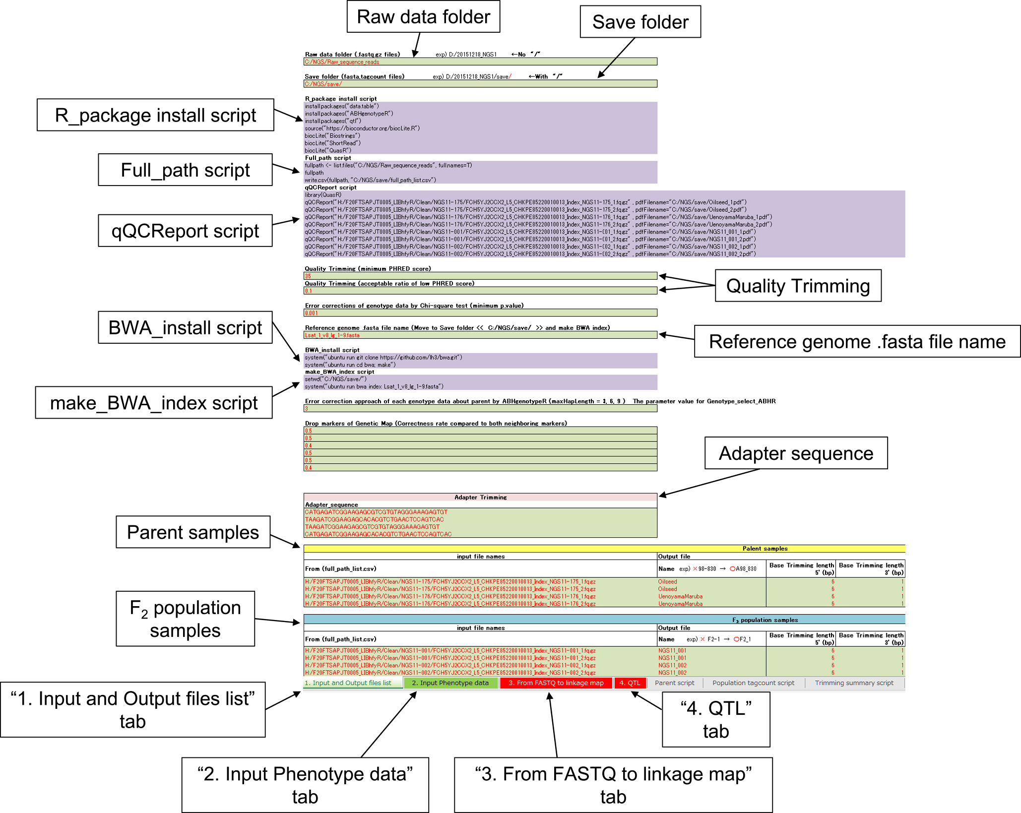
Screenshot of the RAD-R scripts implemented by the Excel software. To set up the script, simply fill in the Information about the specification of the data file and the trimming values in the green cell with the red character of the “1. Input and Output files list” tab.
In the “1. Input and Output files list” tab of the Excel file (Fig. 2), enter the address of the folder containing the raw sequence reads as well as the address of the folder where the analysis data are planned to be saved, based on the entry example. In case of files of the raw sequence read for the parents and the F2 population, enter the full path addresses. A full_path script in purple cells can be used to examine the full path of raw sequence reads. Next, names for the parents and individuals in the F2 population are entered. Since names with only numbers will produce errors, users should use the examples to determine the names. Additionally, an underbar should be used instead of a hyphen. Some green cells have been set up to be able to be chosen from a tab list. It is recommended to run the analysis with the default values of the parameters at first.
The input of the phenotype dataIn the “1. Input and Output files list” tab and “2. Input Phenotype data” tab, the parent and the names of the F2 individuals were linked. Entering phenotype data into the “2. Input Phenotype data” tab, the phe file for R/QTL is automatically created by run RAD-R scripts.
Preparation of reference genome sequence for alignment using BWAReference genome sequences should be saved in the save folder. This R script was designed to make use of the pseudomolecule-level referencing of genome sequences. It can be used for the scaffold-level referencing of genome sequences, although it is not recommended due to the high probability of error in the ABHgenotypeR package (Furuta et al. 2017). If contigs or scaffolds are found to exist in the reference genome sequences, it is advised to remove them from the fasta file of the reference genome sequence beforehand. The R and Burrows-Wheeler Alignment tool (BWA) are used by this pipeline (Li and Durbin 2009). BWA is a Linux-based and BSD-based Mac OS (Unix) software. In the case of Windows10, BWA can run on the Windows System for Linux (WSL). Microsoft’s HP (https://docs.microsoft.com/ja-jp/windows/wsl/install-win10) describes the implementation of WSL. In this script, Ubuntu was adopted. To install the BWA, the BWA_install script should be run with the R console after implementing the WSL. The index files of the reference genome sequence should be created for the BWA by using the make_BWA_index script presented in the purple cells beforehand.
The R packages required for the RAD-R scriptsThe Biostrings package, ShortRead package, QuasR package, data.table package, ABHgenotypeR package, and the qtl package are all required to be installed with the R_package install script presented in the purple cells (Gentleman et al. 2004, R Development Core Team 2017).
Run RAD-R scriptsRAD-R scripts consist of two main R scripts, including the “3. From FASTQ to linkage map” as well as the “4. QTL” that can be easily run by copying and pasting the 19674 lines of R script displayed in the purple cells of the “3. From FASTQ to linkage map” tab into the R console. To perform the QTL analysis, the script of the “4. QTL” tab should be run. Detailed manual and sample data are available at https://github.com/KousukeSEKI/RAD-seq_scripts.
Quality controlThe quality control of the raw sequence reads is necessary as the accuracy of the linkage map is affected by their quality. Raw sequence reads are provided by high-throughput sequencing with a certain percentage of reading errors. Therefore, the PHRED score of the raw sequence reads can be checked by the qQCReport script provided in the purple cells, potentially setting the base trimming of some low-quality sequences of the 5ʹ- and 3ʹ-end (Gaidatzis et al. 2015). The default settings include the trimming of 6 bp of the 5ʹ-end as well as 1 bp of the 3ʹ-end. Besides, it can remove low-quality reads and the adapter sequences from the raw sequence read with the RAD-R scripts. By default, the minimum PHRED score is set to 35 and the acceptable ratio for the low PHRED score is 0.1 (i.e., 10%). The details of the adapter sequence were shown in Fig. 1.
Approaches to linkage map constructionBy comparing the sequence reads in the FASTQ files of the parents, each parent-unique sequence and the common sequences were picked up and three FASTA files were subsequently created. The aligned sequences and positions obtained from the sam files through the alignment of these FASTA files to the reference genome sequence with BWA were saved in the “mappinggenotypelist.csv” file. The mem and aln algorithms were provided in the BWA. From the sam files obtained from each algorithm, two patterns of genotype data were created, one through the application of all the mapped data and the other using only the data with the highest mapping quality. Therefore, the “mappinggenotypelist.csv” file was created in four versions: “mem”, “mem_60”, “aln” and “aln_37”. For each plant in an F2 population, the sequence and the read frequency per sequence were summarized in “name.tagcount” files using the table function. The list of the read frequency for all individual plants about each aligned sequence will were summarized in the “genotypingSum_complete.csv” file by comparing the sequences located in the “name.tagcount” files with those in the “mappinggenotypelist.csv” file using the match function. The “genotypingSum_complete.csv” was considered to be the initial list of genotype data. This pipeline was designed to specifically address F2 populations of the self-fertilization plants, and was not suitable for heterozygous plants. For the dataset of each aligned sequence, the chi-square test was performed for the presence or absence of the read frequency in association with all F2 individual plants as well as datasets of aligned sequences with outliers of p values (3:1) were excluded from the “genotypingSum_complete.csv” file. As the genotype data produced by RAD-seq has a significant amount of missing data in comparison with datasets obtained from genetic markers obtained by conventional methods, the ABHgenotypeR package was adopted to correct errors in the genotype data (Furuta et al. 2017). To achieve better results, three construction methods were provided by this pipeline (Fig. 3).

Schematic view of three construction methods.
1. The datasets of sequences aligned at the same genomic position between parents in the data of the “genotypingSum_complete.csv” file were directly extracted as co-dominant markers and this genotype data was created with the “ABH” notation. The first approach was that the ABHgenotypeR package was run to correct the error of this genotype data. The genotype files obtained in this method were named “Genotype_csvs”.
2. Regarding the data of each parent, the data in association with the reading frequency per genomic position data in the “genotypingSum_complete.csv” file was compared to its neighboring genomic position and subsequently excluded from the data set in case its data pattern differed significantly. This process was repeated three times. The data aligned to the same genomic position between the parents were extracted as co-dominant markers and the selected genotype data was afterwards created with the “ABH” notation. Moreover, each marker in the selected genotype data was re-compared to its neighboring marker and excluded from the selected genotype data in case significant difference in the data pattern. This process was also repeated three times. The second approach was that the ABHgenotypeR package was run to correct the error of these selected genotype data. The genotype files obtained in this method were named “Genotype_select_csvs”.
3. The data of the reading frequency per position data in the “genotypingSum_complete.csv” file was compared to its neighboring position and subsequently excluded from the dataset when its data pattern differed significantly. This process was repeated three times. The ABHgenotypeR package was run to correct the error of this selected dataset per each parent. The parameter of maxHapLength can be selected from 3, 6, and 9. Moreover, the selected data that aligned to the same genomic position between the parents were extracted as co-dominant markers and selected genotype data were created with the “ABH” notation. In addition, each marker in the selected genotype data was re-compared to its neighboring marker and subsequently excluded from the selected genotype data in case of significant difference in its data pattern. This process was also repeated three times. The third approach was that the ABHgenotypeR package was run to correct the error of these selected genotype data. The genotype files obtained in this method were named “Genotype_select_ABHR (maxHapLength)_csvs”.
Two patterns of the error-correction approach by the ABHgenotypeR were set up in which the order of the functions was switched (Fig. 4). “S” means the correctStretches function, and “U” means the correctUndercalledHets function. The parameter of the maxHapLength was set from 1 to 10 for each of the 10 error-corrected csvs files to be created in the save folder. Regarding this RAD-R script, three construction methods were shown in Fig. 3 as well as two correction approaches were depicted in Fig. 4, therefore the total number of combinations included six patterns of genotype data. Besides, as four types of file versions were available based on the mapping quality of the BWA, including “mem”, “mem_60”, “aln”, and “aln_37”, 24 patterns were identified in total. Subsequently, 10 error-corrected csvs files (maxHapLength = 1~10) were created for each pattern, making a total of 240 error-corrected csvs files. The genotype images of these error-corrected csvs files were summarized into 12 PDFs saved in the “Genotype_images_PDF_files” folder to provide an easy method for visually checking the results of each correction approaches. Moreover, duplicate markers with the same genotype data were deleted from each csvs file using the findDupMarkers and the drop.markers functions of the R/QTL package. In addition, the number of markers before and after the deletion of the duplicate markers were summarized in the “Maps_list_(mem and aln).csv” files saved in the “Genotype_images_PDF_files” folder. Using these PDF and CSV files as a reference, genotype data that are more suitable for the QTL analysis can be selected from 240 error-correcting csv files. The names of the genotype data files were indicated by the “mode of BWA (mem, mem_60, aln, and aln_37”, the “construction method (csvs, select, and ABH)” and the “correction approach (the value of maxHapLength plus SU and the US)”.
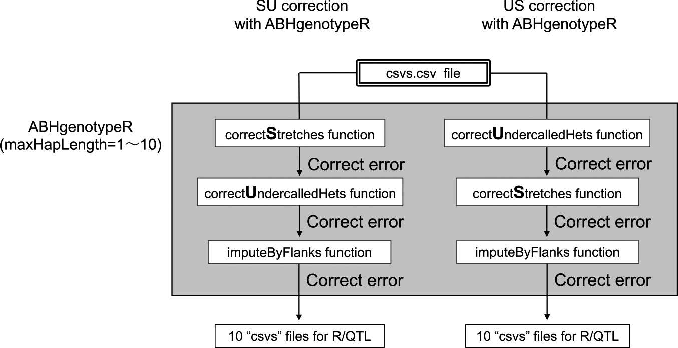
Schematic view of two, SU and US, correction approaches.
In the “4. QTL” tab of the Excel file, in order to select the genotype data file to be analyzed by the R/QTL package (Broman et al. 2003), an appropriate should be selected first as a part of the file name from the four tabs lists settled in green cells. In this way the selected genotype data file would be displayed in the yellow cell. Two visualization functions are offered by the Genotype_Freq_and_Density script along with the physical position of the chromosomes. The plotMarkerDensity function allows the plotting of the density of the markers, whereas the plotAlleleFreq function allows the plotting of the parental allele frequencies. Moreover, the CIM_plot script can provide the visual results of the CIM for all phenotypes. For significant LOD peaks, more detailed results for each locus can be obtained with the Re-CIM_each_Trait script as well as more detailed LOD peak plots can be acquired with the Re-plot script.
Verification testTo demonstrate and illustrate the features of the RAD-R scripts, the publicly available sequence data from the study by Seki et al. (2020) along with the accession number PRJNA523045 (ddRAD-seq) were used for the analysis. The verification test of the RAD-R script was performed using data previously reported on the identification of LsTCP4, a causative candidate gene for marginal leaf shape in lettuce (Seki et al. 2020). Filtered sequence reads were mapped onto the L. sativa v8.0 genome (https://phytozome.jgi.doe.gov/pz/portal.html#!info?alias=Org_Lsativa_er) via the utilization of the mem and the aln modes of the BWA. Using the alignment data associated with these modes, the linkage maps constructed using RAD-R scripts and stacks were compared. The total distance (centimorgan: cM) for the genotype data was calculated using the estimate.map option of the read.cross function in the R/QTL package.
Data availabilityThe reference sequence of Lactuca sativa L. used in this study can be found at Phytozome (DOE-JGI, https://phytozome.jgi.doe.gov/pz/portal.html). The high-throughput sequencing data were deposited to the Sequence Read Archive with the accession number PRJNA523045 (ddRAD-seq).
The percentage of the sequence reads that had the highest mapping quality, namely the “mem_60” and the “aln_37” among those aligned to the reference genome sequence with the BWA were 44.2% and 61.4% in mem and aln modes, respectively (Table 1). The trend was similar for both parents. Without the sequence reads which were not detected in F2 plants, the datasets were reduced from 2078649, 917849, 1607719, and 986689 to 756098 (36.4%), 325665 (35.5%), 693132 (43.1%), and 405243 (41.1%) in “mem”, “mem_60”, “aln”, and “aln_37”, respectively (Table 1). Moreover, the datasets were reduced to 60505 (2.9%), 30102 (3.3%), 64106 (4.0%), and 42937 (4.4%) in “mem”, “mem_60”, “aln”, and “aln_37”, respectively, due to excluded statistical outliers of p values by the chi-square test (Table 1). The summary of the linkage maps constructed was presented in Table 2. Using the RAD-R script, four types of BWA datasets (mem, mem_60, aln, and aln_37) were present, three types of map construction methods (ABH, select, and csv) were identified, and twenty types of error-correction approaches (Each parameter of maxHapLength for SU and US ranges from 1 to 10) were defined, and 240 types of linkage maps could be created. The number of markers ranged from 1954 (mem_60, select) to 5214 (aln, csvs). In regard of the comparison of the linkage maps created by the three construction methods, the number of markers was higher in the order of csv, ABH, and select. In addition, the linkage maps created using stacks had 3908 markers in mem and 3871 markers in aln. The summary of the genotypes of the linkage maps was summarized in Table 3. The minimum and maximum genetic distances after correction were 1269 cM (mem, select, 10US) and 5305.9 cM (aln, csvs, 5US), respectively. In stacks, 15443.7 cM was observed in mem and 16706.6 cM in aln. The linkage maps created using the RAD-R scripts had the missing values in the range of 0.02% to 2.2%, whereas the linkage maps created using stacks had the missing value of 10.44% in mem and 9.89% in aln. The constituted ratio of “A”, “H”, and “B” in each genotype data was compared against the expected ratio of 1:2:1 by goodness-of-fit chi-square tests. Since the all null hypotheses were not rejected, the correction approaches were considered to be appropriate.
| parent | Linkage group | mem | mem_60 | aln | aln_37 | |
|---|---|---|---|---|---|---|
| Number of aligned position to the genome sequence by BWA | P1 | LG1-9 | 1018399 | 464798 | 788105 | 495881 |
| P2 | LG1-9 | 1060250 | 453051 | 819614 | 490808 | |
| Number of datasets without no-count data of F2 plants | P1 | LG1-9 | 365898 | 162612 | 329219 | 197382 |
| P2 | LG1-9 | 390200 | 163053 | 363913 | 207861 | |
| Number of datasets with p-value > 0.001 by chi-square test | P1 | LG1-9 | 30190 | 16743 | 33172 | 23903 |
| P2 | LG1-9 | 30315 | 13359 | 30934 | 19034 |
| In silico analysis | BWA | Construction method | Number of co-dominant marker | |||||||||
|---|---|---|---|---|---|---|---|---|---|---|---|---|
| LG1 | LG2 | LG3 | LG4 | LG5 | LG6 | LG7 | LG8 | LG9 | LG1-9 | |||
| RAD-R scripts | mem | csvs | 639 | 578 | 493 | 215 | 799 | 228 | 284 | 673 | 552 | 4461 |
| select | 425 | 390 | 265 | 58 | 454 | 105 | 134 | 370 | 291 | 2492 | ||
| ABH | 457 | 416 | 300 | 75 | 496 | 116 | 158 | 417 | 355 | 2790 | ||
| mem_60 | csvs | 422 | 391 | 287 | 85 | 530 | 152 | 175 | 404 | 346 | 2792 | |
| select | 343 | 293 | 201 | 46 | 385 | 99 | 99 | 273 | 215 | 1954 | ||
| ABH | 365 | 308 | 228 | 52 | 418 | 106 | 118 | 318 | 251 | 2164 | ||
| aln | csvs | 751 | 632 | 611 | 231 | 912 | 271 | 373 | 753 | 680 | 5214 | |
| select | 497 | 416 | 335 | 74 | 568 | 129 | 181 | 416 | 404 | 3020 | ||
| ABH | 528 | 444 | 377 | 94 | 614 | 143 | 209 | 476 | 462 | 3347 | ||
| aln_37 | csvs | 628 | 543 | 473 | 142 | 769 | 217 | 287 | 604 | 572 | 4235 | |
| select | 516 | 416 | 327 | 80 | 561 | 144 | 177 | 397 | 378 | 2996 | ||
| ABH | 545 | 441 | 367 | 96 | 610 | 153 | 203 | 460 | 451 | 3326 | ||
| Stacks | mem | – | 634 | 534 | 410 | 127 | 735 | 207 | 242 | 551 | 468 | 3908 |
| aln | – | 630 | 511 | 430 | 116 | 704 | 218 | 261 | 544 | 457 | 3871 | |
| In silico analysis | BWA | Construction method | Correction approach | The linkage map | |||||||||||||
|---|---|---|---|---|---|---|---|---|---|---|---|---|---|---|---|---|---|
| No. Marker | Total distance (cM) |
A | H | B | Missing value | Chi-test (1:2:1) | |||||||||||
| No. Genotype | (%) | No. Genotype | (%) | No. Genotype | (%) | No. Genotype | (%) | ||||||||||
| RAD-R scripts | mem | csvs | – | 4461 | 298622.6 | 115070 | 26.87 | 189870 | 44.34 | 113910 | 26.60 | 9406 | 2.20 | 0.643 | |||
| 6US | 5059.3 | 96599 | 22.56 | 236505 | 55.23 | 94663 | 22.10 | 489 | 0.11 | 0.571 | |||||||
| select | – | 2492 | 12690.1 | 65139 | 27.23 | 106627 | 44.57 | 64904 | 27.13 | 2562 | 1.07 | 0.616 | |||||
| 10US | 1269.0 | 59082 | 24.70 | 121379 | 50.74 | 58679 | 24.53 | 92 | 0.04 | 0.988 | |||||||
| ABH | – | 2790 | 10543 | 72619 | 27.11 | 122057 | 45.57 | 71564 | 26.72 | 1600 | 0.60 | 0.709 | |||||
| 10US | 1362.8 | 66413 | 24.80 | 135688 | 50.66 | 65617 | 24.50 | 122 | 0.05 | 0.990 | |||||||
| mem_60 | csvs | – | 2792 | 25650.2 | 74246 | 27.70 | 115481 | 43.08 | 74051 | 27.63 | 4254 | 1.59 | 0.467 | ||||
| 7US | 1410.7 | 66141 | 24.68 | 136027 | 50.75 | 65693 | 24.51 | 171 | 0.06 | 0.988 | |||||||
| select | – | 1954 | 10350 | 51348 | 27.37 | 82770 | 44.12 | 51331 | 27.36 | 2135 | 1.14 | 0.566 | |||||
| 10US | 1301.2 | 46526 | 24.80 | 94764 | 50.52 | 46222 | 24.64 | 72 | 0.04 | 0.994 | |||||||
| ABH | – | 2164 | 6239.3 | 57041 | 27.46 | 93151 | 44.84 | 56261 | 27.08 | 1291 | 0.62 | 0.623 | |||||
| 10US | 1332.4 | 51981 | 25.02 | 104340 | 50.23 | 51290 | 24.69 | 133 | 0.06 | 0.998 | |||||||
| aln | csvs | – | 5214 | 308919 | 134674 | 26.91 | 222555 | 44.46 | 132820 | 26.54 | 10495 | 2.10 | 0.653 | ||||
| 5US | 5305.9 | 115628 | 23.10 | 271817 | 54.30 | 112550 | 22.49 | 549 | 0.11 | 0.681 | |||||||
| select | – | 3020 | 15127 | 78771 | 27.17 | 130051 | 44.86 | 78191 | 26.97 | 2907 | 1.00 | 0.646 | |||||
| 6US | 1370.8 | 71563 | 24.68 | 147459 | 50.86 | 70830 | 24.43 | 68 | 0.02 | 0.984 | |||||||
| ABH | – | 3347 | 9848.8 | 87114 | 27.11 | 147264 | 45.83 | 85141 | 26.50 | 1793 | 0.56 | 0.735 | |||||
| 10US | 1493.1 | 79798 | 24.84 | 163164 | 50.78 | 78182 | 24.33 | 168 | 0.05 | 0.985 | |||||||
| aln_37 | csvs | – | 4235 | 55102.5 | 112032 | 27.56 | 177246 | 43.60 | 111018 | 27.31 | 6264 | 1.54 | 0.524 | ||||
| 5US | 2963.1 | 99899 | 24.57 | 207721 | 51.09 | 98701 | 24.28 | 239 | 0.06 | 0.974 | |||||||
| select | – | 2996 | 15275.8 | 78457 | 27.28 | 128288 | 44.60 | 77848 | 27.07 | 3023 | 1.05 | 0.619 | |||||
| 9US | 1334.6 | 70995 | 24.68 | 146294 | 50.86 | 70261 | 24.43 | 66 | 0.02 | 0.984 | |||||||
| ABH | – | 3326 | 8485.1 | 87106 | 27.28 | 145175 | 45.47 | 85167 | 26.67 | 1848 | 0.58 | 0.694 | |||||
| 10US | 1407.8 | 79488 | 24.89 | 161844 | 50.69 | 77813 | 24.37 | 151 | 0.05 | 0.987 | |||||||
| stacks | mem | – | – | 3908 | 15443.7 | 82644 | 22.03 | 172049 | 45.86 | 81299 | 21.67 | 39176 | 10.44 | 0.566 | |||
| aln | – | – | 3871 | 16706.6 | 82429 | 22.18 | 171188 | 46.07 | 81260 | 21.87 | 36739 | 9.89 | 0.600 | ||||
To validate the accuracy of the genotype data constructed by in silico analysis, QTL mapping with CIM was carried out for the locus of the marginal leaf shape located in LG5. For each mem and aln dataset, a comparison was undertaken in association with the results of the QTL analysis using marker genotype data constructed by the RAD-R scripts and stacks. Although a major LOD peak at the almost appropriate position of LG5 was obtained from all genotype data, the genotype data constructed with stacks was over 1000 cM for mem and 4000 cM for aln even on the LG5 only, and it would not be appropriate to employ this marker genotype data as it is for the QTL analysis. Therefore, to find the genotype data with more appropriate error correction from the 240 genotype data constructed with RAD-R script, the contents of the “Maps_list (mem and aln). csv” and 12 PDF files were subsequently checked. The 12 PDF files that included the images of the genotypes were summarized by varying the value of the parameter of maxHapLength from 1 to 10 in order to facilitate the judgment of the appropriate parameter value in a visual manner. After the review of the content of the PDF files of the “mem” and “aln” data, the correction of the “mem, select, 10US” and “aln, select, 6US” could be visually judged. The genotype data of “aln” was identified to be the most accurate to pinpoint the fine-mapping of the locus of the marginal leaf shape. The results demonstrated that the locus of the leaf marginal serration was located from the 251.599 to the 253.367 Mbp at an interval of 2.1 cM on LG5, as well as the genotype of the RAD marker designated as LG5_v8_252.185_Mbp showed complete co-segregation with the leaf phenotype based on the present F2 population. On the other hand, the results of the “aln” with stacks showed that the locus was located from the 251.386 to the 253.367 Mbp at an interval of 2.6 cM on LG5. The LG5_v8_252.185_Mbp marker was also present in the marker genotype data of the “aln” with stacks, although there were a significant number of missing values resulting in hurdles to identify their complete consistency with the phenotype data. Thus, the results of the validation test showed that the genotype data constructed with the RAD-R scripts could be mapped more accurately than stacks.
R, a free software that is highly reliable and common for users was decided to be used (Broman et al. 2003, R Development Core Team 2017) as it has a wide range of packages to handle not only statistical processing but also biological data, making it suitable for handling big data on nucleotide sequences (Gentleman et al. 2004). Moreover, due to the flexibility of R, the R environment has been established as a versatile and comprehensive platform for the development of the analysis pipeline. The RAD-R scripts are a user-friendly R pipeline that can be implemented using the Excel software and provides an automated flow that could control the quality of raw sequence reads as well as to run, to align, and to reference genome sequences with the BWA, to correct errors by the ABHgenotypeR package, to create 240 error-corrected genotype data, and to perform the QTL analysis. Users without extensive bioinformatics knowledge can easily perform RAD-seq analysis on Windows 10 through the application of the RAD-R scripts.
One of the most important issues in the RAD-seq analysis is that the data produced by high-throughput sequencing has a considerable error-rate. This issue can be dealt with data correction and imputation, that is time-consuming and requires specific bioinformatics awareness. Although the linkage maps constructed with stacks showed high potential, the marker genotype data contained many missing values. Post correction would provide quite accurate genotype data with specialized software, such as TASSEL (Glaubitz et al. 2014), whereas the RAD-R scripts are pipelines that include post correction by default. In this way users are able to perform the analysis in an easier manner. Furthermore, the RAD-R scripts allow the correction of genetic errors, such as unexpected markers in RAD-seq data by the ABHgenotypeR package in order to obtain better results during the QTL analysis. The graphical maps of genotype data created by RAD-R script showed that unexpected markers like biallelic markers that differed in genetic pattern among their neighbor markers were found in multiple genomic positions (Fig. 5). The total distance of the linkage map became enormous due to the abundance of unlinked markers. In the ABHgenotypeR package, the degree of error correction could be adjusted by the value of the maxHapLength parameters. Although the large value of which might reduce the total distance of linkage maps, the error correction may be excessive. With this in mind, during the selection of marker genotype data for the QTL analysis, it is recommended to check the genotype images of the corrected data. By visually validating 12 PDF files containing 240 error-corrected genotype data, users can easily select the appropriate genotype data for the QTL analysis. Besides, the QTL analysis results for the selected genotype data can be quickly obtained with the “4. QTL” script using the R/QTL package.
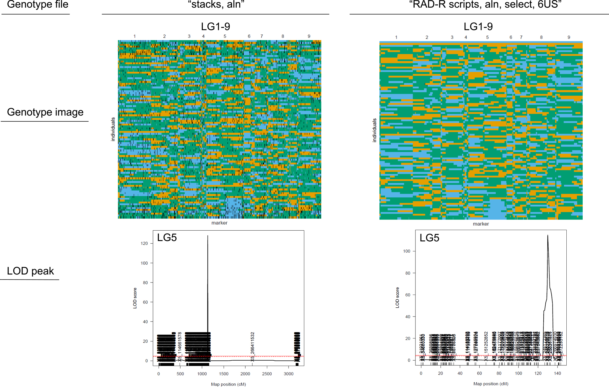
Graphical representations of genotype data constructed by stacks and RAD-R scripts and the LOD plot of the leaf marginal serration locus at LG5 by CIM with R/QTL.
By incorporating the chi-square tests into the pipeline, reads with a low mapping quality of the BWA could be also employed for markers of linkage map construction. This is based on the view that the segregation ratio of the F2 population is more important for the QTL analysis than the mapping quality of the BWA to the reference genome sequence. In this way RAD-R scripts have great potential to contribute to the RAD-seq analysis for the F2 population using parent with a low mapping quality of the BWA, for example the wild type.
In conclusion, a new tool was developed, called RAD-R scripts. This R pipeline would offer fairly reliable genotype data comparable with stacks and can be of use to a large variety of users with limited experience due to the simplicity of copying and pasting R scripts displayed in Excel cells into the R console.
The RAD-R scripts were developed, the data analysis was performed, and the manuscript was written by KS.
The author would like to thank Koji Kadota from The University of Tokyo for disclosing R scripts at the homepage (http://www.iu.a.u-tokyo.ac.jp/~kadota/r_seq.html), Hideo Matsumura from the Gene Research Center, Shinshu University, Hiromi Kajiya-Kanegae from the Research Center for Agricultural Information Technology, National Agriculture and Food Research Organization (NARO), and Ken Naito from the Genetic Resource Center, NARO for supporting the creation of the manuscript with helpful discussions and advices.