Abstract
With the advancement of large-scale omics technologies, particularly transcriptomics data sets on drug and treatment response repositories available in public domain, toxicogenomics has emerged as a key field in safety pharmacology and chemical risk assessment. Traditional statistics-based bioinformatics analysis poses challenges in its application across multidimensional toxicogenomic data, including administration time, dosage, and gene expression levels. Motivated by the visual inspection workflow of field experts to augment their efficiency of screening significant genes to derive meaningful insights, together with the ability of deep neural architectures to learn the image signals, we developed DTox, a deep neural network-based in visio approach. Using the Percellome toxicogenomics database, instead of utilizing the numerical gene expression values of the transcripts (gene probes of the microarray) for dose-time combinations, DTox learned the image representation of 3D surface plots of distinct time and dosage data points to train the classifier on the experts’ labels of gene probe significance. DTox outperformed statistical threshold-based bioinformatics and machine learning approaches based on numerical expression values. This result shows the ability of image-driven neural networks to overcome the limitations of classical numeric value-based approaches. Further, by augmenting the model with explainability modules, our study showed the potential to reveal the visual analysis process of human experts in toxicogenomics through the model weights. While the current work demonstrates the application of the DTox model in toxicogenomic studies, it can be further generalized as an in visio approach for multi-dimensional numeric data with applications in various fields in medical data sciences.
INTRODUCTION
Toxicogenomics is the study of molecular events in the living system induced by the chemical agents entering the system. Its goal is to comprehensively elucidate the molecular mechanisms that lead to toxicological adverse events, and subsequently improve the diagnostics, treatment for known toxicants, and prediction of toxicity for newly made chemicals by the modern technologies for the purpose of better living. With the advancements in the large-scale omics technologies and drug-treatment data repositories available in public domain, toxicogenomics has emerged as a key field in the safety pharmacology and risk assessment (Barel and Herwig, 2018). Several toxicogenomics databases have been developed, including Comparative Toxicogenomics Database (Davis et al., 2021), TG-gates (Igarashi et al., 2015) and Toxygates (Nyström-Persson et al., 2013). The Percellome database (Kanno et al., 2006) is one of the pioneering databases of the field that provides genome-wide absolute mRNA expression levels per cell from various organs of mice that are exposed to a variety of chemical compounds.
Identifying the key responsive molecules upon exposure to a chemical compound over multiple doses and time-points is critical for the assessment of underlying mechanisms of the potential toxicity of the chemicals. For example, comprehensive analysis of the Percellome data for Pentachlorophenol (PCP) revealed that PCP is highly likely to induce hyperthermia through strong activation of interferon signaling pathways (Kanno et al., 2013). Under the administration of chemical compounds, genes often show non-linear complex dynamics in their expression levels across dose and time. The use of classical bioinformatics methods such as differentially expressed gene (DEG) analysis alone is likely to be insufficient to capture all potentially affected important genes. Expert researchers in the toxicogenomics field thus augment the bioinformatics analysis by visually inspecting the 3D-surface image for each single probe which shows the dose- and time-dependent changes in gene expression induced by chemical compounds (Kanno et al., 2013). However, the large volume and complexity of the 3D-surface image datasets make such visual-inspection process time-consuming and labor-intensive. Our motivation in this study is to develop a ‘Toxicologists’ lens’- an automated and efficient in visio visual analysis pipeline that computationally inspects the high dimensional data space across large-scale gene panels and time- and dose-dependent data points.
Rapid progress in the fields of artificial intelligence has opened new avenues for their applications in different domains, particularly in biomedicine and healthcare. Specifically, development of computer vision techniques, driven by deep neural network (DNN) methods, has further augmented biomedical imaging applications. Convolutional neural networks (CNNs) are part of DNN architectures which are designed to learn representation at different levels of abstraction from input signals. A CNN automatically extracts features that reflect high-order statistics of images and utilizes them to accurately classify the images (Esteva et al., 2021). While many challenges exist to fully exploit CNNs on biomedical data such as high data dimensionality and heterogeneity, recent studies have applied CNNs in medical imaging in classification and segmentation problems, particularly in areas of radiology, pathology, ophthalmology and related disciplines (Esteva et al., 2021; Seddiki et al., 2020; Litjens et al., 2017). These methods have also been adopted in computational toxicological studies for toxicity evaluation and prediction by learning from multi-modal features of compounds and the underlying biology (Vo et al., 2020; Pu et al., 2019; Mayr et al., 2016). The availability of large-scale screening data on environmental chemicals and drugs, as in the Tox21 data set (Mayr et al., 2016), has paved the way for multi-task learning of various toxicological effects from CNN architectures (Yuan et al., 2019).
Motivated by the needs of visual data inspection workflow by experts and the ability of CNN architectures, we developed Dtox, an in visio model to evaluate and identify significant genes associated with chemical compound exposure. Using microarray data in the Percellome database, instead of inputting the quantified numerical values of the transcripts (gene probes) for dose-time combinations, Dtox transforms the data into 3D surface plots for gene probes. The model is then trained on the images to identify significant gene probes which were visually labeled by experts.
Dtox outperformed existing data analytic pipelines using DEG analysis as well as traditional machine learning techniques on numerical data. Together with an explainability module to identify the key features in the images, Dtox provides a glass-box model to improve the workflow of toxicologists and accelerate the analysis of large-scale toxicogenomics data.
MATERIALS AND METHODS
Training image dataset
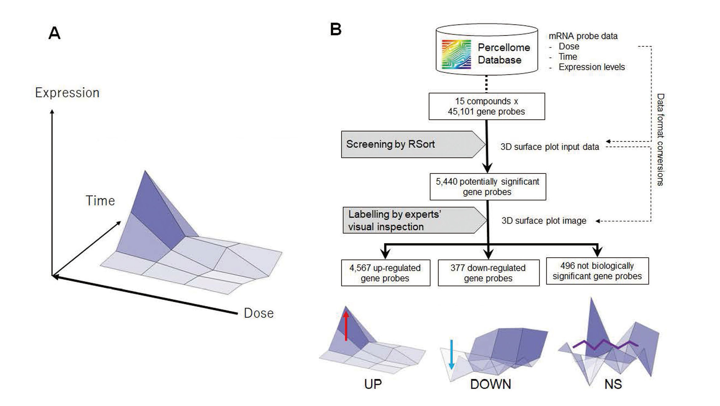
For each mRNA probe data, we generated 10 3D-surface images for each probe taken from ten different angles where the x and y axes are dose and time points and the z-axis represents mean gene expression level for three replicates. The final training dataset consists of a total of 5,440 3D-surface images including angle variations that comprise 4,567 images for up-regulated, 377 images for down-regulated, and 496 images for not-biologically-significant (N.S.) classes.
Convolutional Neural Network (CNN) model
DTox employs Resnet-18 deep learning architecture (He et al., 2016) for image classification tasks. Resnet-18 is composed of 17 convolutional layers, 17 batch normalization layers, 17 activation layers using Rectified Linear Unit (ReLU) (Nair and Hinton, 2010) activation function, one input layer, one max pooling layer, one average pooling layer, one flatten layer, one dense layer, and shortcut links (see Supplementary Table 1 for details). Through the input layer to the flatten layer, the Resnet-18 generated 512 features for each image. The final dense layer used these 512 features to classify genes into three classes, i.e., UP class, DOWN class, and N.S. class. Resnet-18 was implemented by using two python modules, i.e., torch version 1.12.1+cu102 and torchvision version 0.13.1+cu102. In optimization of weights in Resnet-18 (He et al., 2016), gradient optimization with the Adam optimizer was performed. In the model training step, we set the number of epochs as 100 and batch size as 32 while default values were used for other parameters. In the optimization step, we minimized categorical cross-entropy loss between predicted and actual labels. The model was trained and executed on the computational server with NVIDIA Tesla V100.
Differential Gene Expression (DEG) analysis in the Bioinformatics pipeline
In DEG analysis, mRNA expression values were log2 transformed and Welch’s T-test (t.test in R) plus multiple testing correction with Benjamini-Hochberg (p.adjust in R) were calculated to identify genes that are significantly up- or down-regulated under time and dose combinations against control vehicle conditions. At each time point (e.g., 8 hr), we compared gene expression levels of a probe set under 3 compound dosages (low, middle and high dosages) with those under the control condition without compound exposures (vehicle control). Genes with log2 absolute fold-change > 1 and various adjusted p-value by Welch’s T-test with Benjamini-Hochberg’s multiple-testing correction were applied to detect significantly up- or down-regulated genes.
Machine learning pipeline
We used XGBoost (Chen and Guestrin, 2016) and Random Forest (Breiman, 2001) as state-of-the art machine learning algorithms to classify probes into informative (up- or down-regulated) probes or non-informative probes based on 48 numerical values as input features. The models were built using python module scikit-learn (Pedregosa et al., 2011) version 1.2.2 and xgboost version 1.7.6 and evaluated by 5-fold cross validation. In XGBoost modeling, grid search examined combinations of various hyper-parameters to fit the model; learning_rate = (0.3, 0.4), max_depth = (2, 3, 5, 10), booster = (‘gbtree’), objective=('multi:softprob'), reg_lambda = (0.01, 1, 20), reg_alpha = (0.01, 1, 20), and n_estimators = (10, 100). The default values were used for the other tuning parameters. In RandomForest modeling, we fit the model by examining various parameters; max_depth = (2, 3, 5, 10), min_samples_split = (2, 3, 5, 10), criterion = ('gini', 'entropy'), max_features = ('sqrt', 'log2'), and _n_estimators = (10, 100), while the other tuning parameters set as default.
Grad-cam in explainability analysis
We implemented XGrad-CAM (Fu et al., 2020) with XGradCam function in torchcam module version 0.4.0 (https://frgfm.github.io/torch-cam/) to assess gradients activated by classes associated with input 3D-surface images. We traced the gradients flow into the last convolution layers for the last residual block in Resnet18 (layer4, see Supplementary Table 1) and highlighted them on pixels in the 3D-surface images.
RESULTS
In this section, we outline the results of the Dtox deep neural-network model, to classify significant genes under the effect of chemical compounds based on 3D-surface images transformed from classical numerical data (dose-time transcriptomics data for toxicology). We compared the classification performance of Dtox with traditional bioinformatics analysis as well as classical machine learning models that use the original numerical data for their classification tasks. Furthermore, we elucidate the model results with an explainability method to get an insight into how Dtox models classify significant genes.
Transformation of microarray gene-probe data into 3D-surface image
The Percellome database provides toxicogenomics data for 160 chemical compounds measured by the Affymetrix GeneChip MOE430 2.0 microarray under the combination conditions of 4 dose level and 4 time points. For each of the 16 dose-time combination conditions, 3 mice were used to measure mRNA expression for each gene. Therefore, gene expression data for each gene is composed of 48 (16 dose-time point combinations for 3 mice samples) numerical values of gene expression. In addition to the numerical values for each compound and probe set, the database also provides a 3D-surface image for each probe for the ease of visual inspection of the impact of the compound exposure in absolute gene expression (Fig. 1). In the 3D surface plot, the x, y, and z axes represent dose (4 dose levels: vehicle, low, middle, and high dose levels), time points (4 time points: 2, 4, 8, 24 hr), and the mean expression level among three replicate samples for a gene probe, respectively (Fig. 1A). Each compound measures 45,101 probes that undergo experts’ inspection as part of the toxicogenomics research workflow to comprehensively identify significant genes and pathways. The Percellome 3D-graph visualization tool allows users to rotate and turn the 3D-surface images so that the experts can check the image from various angles during visual inspection.
We used Percellome transcriptome datasets of 15 tested chemical compounds each of which contains 45,101 3D-surface images for corresponding gene probes. The comprehensive experts’ visual selection of the up- or down-regulated mRNA probe sets that responded to the administration of the test chemical was performed in two steps.
First, probe screening is made by an in-house program named RSort (Kanno et al., 2013). RSort sorts the 3D-surfaces by their roughness in shape based on the number of peaks on the 4 x 4 grid of each surface. The upward and downward peaks are iteratively detected by picking one data point with the largest difference from the average of all data points where the neighbors of that data point on the 3D-surface showing similar expression levels to that data point (difference < 0.5 × SD are merged into the same peak and these peakcs) will be eliminated for the next iteration. This iteration gives the number of peaks from one to eight.
It then selects the probes with less than three peaks (this cut-off value can be changed in certain cases). The probes with maximum expression lower than 2 copies per cell are discarded. Student’s t-test between the mRNA values of vehicle control and treated groups of each time point is calculated and probes with at least one point with p < 0.05 are retained. These steps by RSort selected 5,440 probes as potentially important genes to be explored in the next visual inspection step.
Second, the probes are further selected by visual inspection on 3D-surface images. It is based on several biological assumptions on time-course and dose-response of the mRNA in in vivo organs to pick up the cascade of biological events triggered by the single administration of a test chemical substance. For example, the fastest response of mRNA to a chemical is known to become monitorable on the order of 10 min and assumed to be monitored as a transient wave at 2 hr or later in our experimental protocol. This assumption is based on the analysis that the mRNA responses are lognormal in time (Konishi, 2004, 2005). Second or third rounds of genes that are indirectly induced by the chemical should follow the first wave of mRNAs and, indeed they are monitored at 4, 8, or 24 hr after administration as reported elsewhere (Kanno et al., 2006, 2013). In terms of dose-response, the dose range adopted by the Percellome Project is 0, 1, 3, and 10, which is biologically narrow in range and the dose-response is well predicted to be monotonous within this range, including patterns of saturation from any dose levels. Based on the time and dose range of the data mentioned above, it is assumed that biologically responding genes can be monitored as one wave or at most two waves made of monotonous dose-response slope in 3D-surface graphs that have a maximum of two significant peaks. Experts browse the shape of 3D-surfaces of probes pre-selected by the RSort program and pick up probes that fulfill these biologically assumed characteristics.
Based on the above experts’ routine procedure, each of the 5,440 3D-surface images was labeled into three classes: UP-regulated (4,567 images), DOWN-regulated (377 images), and Not biologically significant (N.S.) (496 images) (Fig. 1B).
Bioinformatics pipeline-based key gene prediction
Differential Gene Expression (DEG) analysis of the 5,440 gene probes was performed as a benchmark of a traditional bioinformatics pipeline to identify key genes that show statistically significant expression changes under each of three doses at each time point against control (vehicle) conditions. Probes were then classified into four classes based on DEG analysis results, UP, DOWN, NS, and MIX classes by the following criteria:
- UP: significantly upregulated in at least one condition and not downregulated in any condition
- DOWN: significantly downregulated in at least one condition and not upregulated in any condition
- NS (not statistically significant): genes are not up- and down-regulated in all conditions
- MIX: up-regulated in at least one condition and down-regulated in at least one condition.
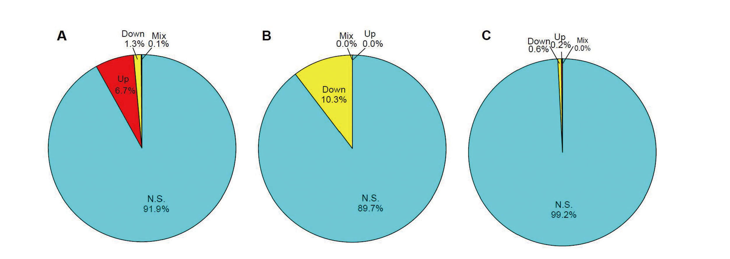
The DEG-based probe classification results were compared with those from experts’ visual inspection (Table 1 and Fig. 2). The class prediction result for each of the training probe sets is provided in Supplementary Table 2. As demonstrated in the figure, the DEG-based analysis tends to predict probes as N.S. and can identify only 9 and 11 percent of genes under UP and DOWN-regulated genes from experts’ visual inspection, respectively.
Table 1. Comparison between Experts’ labeling and DEG-based prediction with the threshold of p < 0.05.
|
DEG-based prediction (# probes) |
Total# probes |
| UP |
Down |
MIX |
NS |
Experts’ label
(# probes) |
UP |
304 |
59 |
6 |
4198 |
4567 |
| DOWN |
0 |
39 |
0 |
338 |
377 |
| Biologically NS |
1 |
3 |
0 |
492 |
496 |
| Total # probes |
305 |
101 |
6 |
5028 |
5440 |
Most of the gene probes were judged as “non-statistically significant (NS)” with the threshold of p < 0.05. Interestingly, 59 gene probes which were labelled as UP-regulated gene probes by experts were judged as DOWN group in the DEG-based analysis with p < 0.05. Also, a few gene probes with the biologically non-significant label were judged as UP or DOWN groups in the DEG analysis.
DTox: Deep learning based classifier model building
We next constructed a CNN model (named as DTox) using Resnet-18 architecture (Supplementary Table 1) which extracts features embedded in 3D-surface images of gene probes and uses the features to classify gene probes into three classes, UP-regulated, DOWN-regulated, and non-biologically significant (NS) (Fig. 1B). The construction and evaluation of DTox is composed of 3D image data preprocessing, CNN model training, and the assessment of predictive performance against test dataset as well as by comparison of other methodologies. The preprocessing of 3D-surface images was performed by the following procedures: (1) Ten images for each gene probe in different angles were generated in the Percellome database (Supplementary Table 3 and Supplementary Fig. 1), (2) The visual information other than the 3D-surface that become the source of noise, such as axis lines and gene names plotted in routine procedure for the purpose to give gene information to the experts, were removed from each image, and (3) These images were cropped to 500*500 pixels and converted into RGB color scales. The images were resized into 224*224 pixels images and used for training deep learning models.
DTox was then built to select informative genes based on a residual learning framework, ResNet, composed of a larger number of layers, mainly 17 convolutional layers, together with identity shortcut connections (He et al., 2016). The identity shortcut connections enable Resnet models to skip a few layers that cause predictive performance degradations so that the model can achieve high prediction accuracy in image classification tasks. Ten distinct classifier models associated with ten different angles (see Supplementary Fig. 1 and Supplementary Table 3) were independently tuned. The Resnet models automatically extract features from image data through multiple convolutional layers, shortcut connections, and the fully connected layer in the models. The output layer in the Resnet models use the features to classify each gene into three classes, UP, DOWN, and N.S. classes. The predictive performance assessment of DTox for each angle was done by five-fold cross validation and represented in three-by-three confusion matrices to calculate evaluation metrics for each fold and mean values of the metrics among the five folds.
Comparative evaluation
In order to benchmark the performance of the DTox models, systematic performance analysis was performed together with the assessment of the bioinformatics analysis pipeline and classical machine learning models using Random Forest and XGBoost frameworks to classify the probes into three classes based on the numerical values of 16 time-dose combinations as an input feature (see Materials and Methods for details).
Table 2 shows Accuracy, Kappa, Sensitivity, and Specificity scores calculated for ten independent DTox models based on ten different angles of 3D-surface images, DEG-based bioinformatics pipeline and the machine learning models. The ten DTox models from different angles show comparable classification accuracies ranging as high as 0.984 to 0.992 in Accuracy and 0.940 to 0.973 in Kappa. These results are likely to ensure high predictive performance and robustness of DTox classifiers.
Table 2. Assessment of prediction accuracies of DTox and other pipelines.
| Method |
Accuracy |
Kappa |
Sensitivity (Up) |
Sensitivity (Down) |
Specificity (Up) |
Specificity (Down) |
| DTox (angle1) |
0.989 (0.004) |
0.962 (0.016) |
0.995 (0.003) |
0.973 (0.013) |
0.971 (0.017) |
0.997 (0.003) |
| DTox (angle2) |
0.984 (0.021) |
0.940 (0.076) |
0.997 (0.002) |
0.963 (0.035) |
0.954 (0.058) |
0.993 (0.012) |
| DTox (angle3) |
0.991 (0.004) |
0.968 (0.014) |
0.997 (0.001) |
0.963 (0.024) |
0.971 (0.014) |
0.998 (0.002) |
| DTox (angle4) |
0.991 (0.002) |
0.968 (0.007) |
0.996 (0.003) |
0.973 (0.025) |
0.978 (0.008) |
0.997 (0.002) |
| DTox (angle5) |
0.990 (0.002) |
0.966 (0.009) |
0.995 (0.002) |
0.971 (0.022) |
0.979 (0.011) |
0.997 (0.002) |
| DTox (angle6) |
0.990 (0.005) |
0.965 (0.018) |
0.995 (0.006) |
0.976 (0.026) |
0.983 (0.012) |
0.996 (0.003) |
| DTox (angle7) |
0.991 (0.003) |
0.967 (0.012) |
0.996 (0.002) |
0.976 (0.026) |
0.978 (0.015) |
0.996 (0.002) |
| DTox (angle8) |
0.992 (0.003) |
0.973 (0.012) |
0.997 (0.002) |
0.973 (0.016) |
0.981 (0.009) |
0.997 (0.002) |
| DTox (angle9) |
0.988 (0.006) |
0.958 (0.020) |
0.995 (0.004) |
0.968 (0.031) |
0.969 (0.023) |
0.994 (0.006) |
| DTox (angle10) |
0.991 (0.003) |
0.968 (0.012) |
0.997 (0.003) |
0.979 (0.013) |
0.981 (0.017) |
0.996 (0.003) |
| Bioinformatics (p < 0.05) |
0.153 |
0.024 |
0.067 |
0.103 |
0.999 |
0.988 |
| Bioinformatics (p < 0.1) |
0.184 |
0.036 |
0.101 |
0.143 |
0.998 |
0.984 |
| Bioinformatics (p < 0.2) |
0.227 |
0.052 |
0.148 |
0.210 |
0.993 |
0.982 |
| Bioinformatics (p < 0.3) |
0.250 |
0.062 |
0.173 |
0.265 |
0.989 |
0.980 |
| Bioinformatics (p < 0.4) |
0.271 |
0.068 |
0.199 |
0.289 |
0.982 |
0.976 |
| Bioinformatics (p < 0.5) |
0.282 |
0.069 |
0.203 |
0.302 |
0.983 |
0.973 |
| Bioinformatics (p < 0.6) |
0.276 |
0.066 |
0.210 |
0.302 |
0.977 |
0.970 |
| Random Forest |
0.914 (0.006) |
0.614 (0.040) |
0.996 (0.003) |
0.231 (0.051) |
0.496 (0.052) |
0.998 (0.002) |
| XGBoost |
0.953 (0.003) |
0.818 (0.013) |
0.992 (0.003) |
0.637 (0.038) |
0.770 (0.020) |
0.994 (0.002) |
Note that the numbers outside/in parenthesis represent mean/standard deviation values were calculated and displayed from five test datasets used in 5-fold cross validation for the results of DTox, XGBoost, and Random Forest. For Bioinformatics analysis, the numbers represent performance metrics calculated from all the 5,440 probes.
In the assessment of the classification performance of the DEG-based bioinformatics analysis, we regarded probes in MIX category as those in N.S. category while the number of probes in MIX category is less than 0.1% of total probes and the impacts of these probes on prediction performance score were negligible. In the assessment, we examined the DEG-based bioinformatics analysis with p-value threshold of 0.05, 0.1, 0.2, 0.3, 0.4, 0.5, and 0.6. As a result, the DEG-based bioinformatics analysis with the statistical threshold of p < 0.5 showed higher accuracy and kappa than that with p < 0.05, p < 0.1, p < 0.2, p < 0.3, p < 0.4, and p < 0.6. However, accuracy and kappa of DEG-based bioinformatics analysis with p < 0.5 are very low, i.e., 0.282 and 0.069, respectively.
As demonstrated in Table 2, both classical machine learning models of Random Forest and XGBoost based on numerical data points showed 0.913 and 0.953 in Accuracy, respectively, which are comparable with DTox. However, the Kappa scores were 0.614 and 0.818 that were lower than those of DTox classifiers. Especially the sensitivity of detection of DOWN class was limited in the machine learning-based classifiers (0.231 for Random Forest and 0.637 for XGBoost). These results indicate that experts visually pick up various trends in down-regulated probes which were not fully represented in numerical vectors and only DTox classification models could replicate such human visual inspection.
Explainability of DTox
To address the explainability of the DTox classifiers, we utilized a state-of-the-art expandability algorithm, X-Gradient-weighted Class Activation Mapping (XGrad-Cam) (Fu et al., 2020), that provides better visualization performances than original Grad-CAM (Selvaraju et al., 2017). The XGrad-CAM on DTox uses average of gradients for weight of activation maps (pixels) and its effect on the last convolutional layer of the last residual block (Resnet18 composed of four residual block layers as shown in Supplementary Table 1, i.e., in order of proximity to the input layer, layer1, layer2, layer3, and layer4) in the Resnet18 model to classify the images into three classes. The representative images of highlighted pixels by XGrad-Cam were shown in Figs. 3 and 4 for angle 1 and angle 6, respectively, where angle 1 is the default angle for the 3D plot images (see Supplementary Fig. 1) and angle 6 shows the highest specificity for Up class among the 10 angle models (Table 2). In each plot, the deeper red and deeper blue pixels represent more and less responsible for the predictions, respectively. In Fig. 3 and Fig. 4, panel A shows the XGrad-Cam result for example probes in UP class and panel B for the probes in DOWN class, respectively.

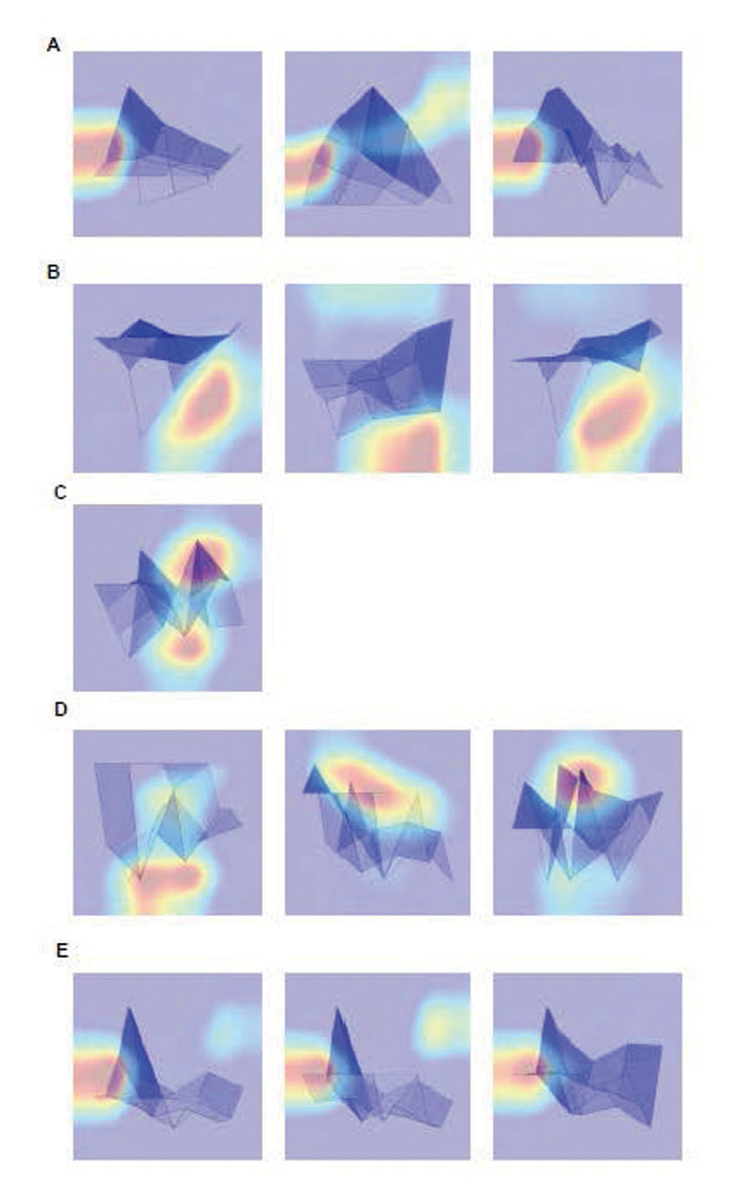
The XGrad-Cam highlights the leading and tailing edges of peaks of the graph images. It is pertinent to note here that the human experts also focus on such edges of peaks in the images to classify UP or DOWN genes. Panel C and D show the probes in NS class but bioinformatics pipeline (FC > 1, adjusted p < 0.05) mislabeled as UP and DOWN, respectively, whereas the XGrad-Cam highlights multiple peaks so that DTox correctly detects these probes as NS. Panel E shows the probes in UP class, but bioinformatics pipeline (FC > 1, adjusted p < 0.05) mislabeled the probe as DOWN, where as the XGrad-Cam highlights both edge slope of the peak and the followed by flat part and DTox correctly detects these probes as UP. These results indicate that the DTox model have potential to capture experts’ visual inspection techniques.
DISCUSSION
In imaging classification such as skin cancer patients’ diagnosis (Esteva et al., 2017), Alzheimer’s disease pathology classification (Tang et al., 2019), cingulate island sign detection in dementia (Iizuka et al., 2019) and eye disease detection (Babenko et al., 2022), the success of CNN-based applications replicating biomedical domain experts has been remarkable. In addition, there recently have been attempts to apply a CNN framework to analyze numerical data, for example, DeepInsight (Sharma et al., 2019) transformed a set of numerical features vectors into image data by dimensional reduction techniques and built a CNN model based on the transformed and amplified images. DeepInsight successfully classified ten cancer types using their RNAseq data and demonstrated higher classification accuracy compared to the conventional off-the-shelf machine learning methods. Further, DeepInsight-3D (Sharma et al., 2023) transformed multi-omics data into colored images and, by using CNN models trained with the resultant image data, successfully predicted anti-cancer drug responses of individual patients.
In this work, we have proposed the DTox model framework that replicates experts’ visual inspections in toxicology using 3D-surface image datasets transformed from numerical data which represent time and dose dependencies. Dtox suggests us a set of significant genes under the effect of different chemical compounds which can be further analyzed with such as pathway enrichment analysis and ontology analysis.
Our results lead to several key observations. First, traditional approaches on the numerical and multi-dimensional toxicogenomic data (time+dose) including DEG-based bioinformatics analysis and classical machine learning models are likely to miss genes which are potentially involved in toxicological insights. Second, experts in the field regularly augment their analysis workflow by visual inspection of the data to derive meaningful insights. Third, DTox developed as a computer vision “lens” to enable the in visio analysis of the toxicogenomics data showed the ability of image-driven neural networks to overcome the limitations of numerical data-based approaches. And finally, by augmenting the DTox model with explainability modules, we provide a computational lens to reveal how human experts judge the significance of the gene in the particular toxicogenomics data analysis.
Taken together, these results show the potential of accelerating computational toxicology pipelines by leveraging the deep learning architectures in novel ways, in this case, by transforming numerical data into 3D images and learning representations from them. The DTox model has the potential to increase the efficiency of toxicologists and to be used as an interpreter by providing an assistive lens of explainability. While the current work focuses on the application of the DTox model in toxicogenomic studies, it can be further expanded and generalized as an AI-based visual inspection concept for multi-dimensional numeric data, which can be applied to various fields in medical data sciences.
ACKNOWLEDGMENTS
The super-computing resource was provided by Human Genome Center, the Institute of Medical Science, the University of Tokyo. HK is supported by the COI-NEXT Program to OIST by Japan Science and Technology Agency (JST).
Code availability
All the models and codes to replicate this study are publicly available in Github (https://github.com/TakeshiHase/DTOX).
Funding
This study was supported by Health Sciences Research Grants H30-Kagaku-Shitei-001 and 21KD2001 from the Ministry of Health, Labour and Welfare, Japan.
Conflict of interest
The authors declare that there is no conflict of interest.
REFERENCES
- Babenko, B., Mitani, A., Traynis, I., Kitade, N., Singh, P., Maa, A.Y., Cuadros, J., Corrado, G.S., Peng, L., Webster, D.R., Varadarajan, A., Hammel, N. and Liu, Y. (2022): Detection of signs of disease in external photographs of the eyes via deep learning. Nat. Biomed. Eng., 6, 1370-1383.
- Barel, G. and Herwig, R. (2018): Network and Pathway Analysis of Toxicogenomics Data. Front. Genet., 9, 484.
- Breiman, L. (2001): Random Forests. Mach. Learn., 45, 5-32.
- Chen, T. and Guestrin, C. (2016): XGBoost: A Scalable Tree Boosting System. In: Proceedings of the 22nd ACM SIGKDD International Conference on Knowledge Discovery and Data Mining. KDD, 16, 785-794. Association for Computing Machinery, New York.
- Davis, A.P., Grondin, C.J., Johnson, R.J., Sciaky, D., Wiegers, J., Wiegers, T.C. and Mattingly, C.J. (2021): Comparative Toxicogenomics Database (CTD): update 2021. Nucleic Acids Res., 49 (D1), D1138-D1143.
- Esteva, A., Chou, K., Yeung, S., Naik, N., Madani, A., Mottaghi, A., Liu, Y., Topol, E., Dean, J. and Socher, R. (2021): Deep learning-enabled medical computer vision. npj. Digit. Med., 4, 1-9.
- Esteva, A., Kuprel, B., Novoa, R.A., Ko, J., Swetter, S.M., Blau, H.M. and Thrun, S. (2017): Dermatologist-level classification of skin cancer with deep neural networks. Nature, 542, 115-118.
- Fu, R., Hu, Q., Dong, X., Guo, Y., Gao, Y. and Li, B. (2020): Axiom-based grad-cam: Towards accurate visualization and explanation of cnns. arXiv preprint arXiv:2008.02312.
- He, K., Zhang, X., Ren, S. and Sun, J. (2016): Deep Residual Learning for Image Recognition., pp. 770-778.
- Igarashi, Y., Nakatsu, N., Yamashita, T., Ono, A., Ohno, Y., Urushidani, T. and Yamada, H. (2015): Open TG-GATEs: a large-scale toxicogenomics database. Nucleic Acids Res., 43, D921-D927.
- Iizuka, T., Fukasawa, M. and Kameyama, M. (2019): Deep-learning-based imaging-classification identified cingulate island sign in dementia with Lewy bodies. Sci. Rep., 9, 8944.
- Kanno, J., Aisaki, K., Igarashi, K., Kitajima, S., Matsuda, N., Morita, K., Tsuji, M., Moriyama, N., Furukawa, Y., Otsuka, M., Tachihara, E., Nakatsu, N. and Kodama, Y. (2013): Oral administration of pentachlorophenol induces interferon signaling mRNAs in C57BL/6 male mouse liver. J. Toxicol. Sci., 38, 643-654.
- Kanno, J., Aisaki, K., Igarashi, K., Nakatsu, N., Ono, A., Kodama, Y. and Nagao, T. (2006): “Per cell” normalization method for mRNA measurement by quantitative PCR and microarrays. BMC Genomics, 7, 64.
- Konishi, T. (2005): A thermodynamic model of transcriptome formation. Nucleic Acids Res., 33, 6587-6592.
- Konishi, T. (2004): Three-parameter lognormal distribution ubiquitously found in cDNA microarray data and its application to parametric data treatment. BMC Bioinformatics, 5, 5.
- Litjens, G., Kooi, T., Bejnordi, B.E., Setio, A.A., Ciompi, F., Ghafoorian, M., van der Laak, J.A., van Ginneken, B. and Sánchez, C.I. (2017): A survey on deep learning in medical image analysis. Med. Image Anal., 42, 60-88.
- Mayr, A., Klambauer, G., Unterthiner, T. and Hochreiter, S. (2016): DeepTox: Toxicity Prediction using Deep Learning. Front. Environ. Sci., 3, 80.
- Nair, V. and Hinton, G.E. (2010): Rectified linear units improve restricted boltzmann machines. In: Proceedings of the 27th International Conference on International Conference on Machine Learning, ICML’10, pp. 807-814, Omnipress, Madison, Madison, Wisconsin.
- Nyström-Persson, J., Igarashi, Y., Ito, M., Morita, M., Nakatsu, N., Yamada, H. and Mizuguchi, K. (2013): Toxygates: interactive toxicity analysis on a hybrid microarray and linked data platform. Bioinformatics, 29, 3080-3086.
- Pedregosa, F., Varoquaux, G., Gramfort, A., Michel, V., Thirion, B., Grisel, O., Blondel, M., Prettenhofer, P., Weiss, P., Dubourg, V., Vanderplas, J., Passos, A., Cournapeau, D., Brucher, M., Perrot, M. and Duchesnay, E. (2011): Scikit-learn: Machine Learning in Python. J. Mach. Learn. Res., 12, 2825-2830.
- Pu, L., Naderi, M., Liu, T., Wu, H.-C., Mukhopadhyay, S. and Brylinski, M. (2019): eToxPred: a machine learning-based approach to estimate the toxicity of drug candidates. BMC Pharmacol. Toxicol., 20, 2.
- Seddiki, K., Saudemont, P., Precioso, F., Ogrinc, N., Wisztorski, M., Salzet, M., Fournier, I. and Droit, A. (2020): Cumulative learning enables convolutional neural network representations for small mass spectrometry data classification. Nat. Commun., 11, 5595.
- Selvaraju, R.R., Cogswell, M., Das, A., Vedantam, R., Parikh, D. and Batra, D. (2017): Grad-CAM: Visual Explanations From Deep Networks via Gradient-Based Localization., pp. 618-626.
- Sharma, A., Vans, E., Shigemizu, D., Boroevich, K.A. and Tsunoda, T. (2019): DeepInsight: A methodology to transform a non-image data to an image for convolution neural network architecture. Sci. Rep., 9, 11399.
- Sharma, A., Lysenko, A., Boroevich, K.A. and Tsunoda, T. (2023): DeepInsight-3D architecture for anti-cancer drug response prediction with deep-learning on multi-omics. Sci. Rep., 13, 2483.
- Tang, Z., Chuang, K.V., DeCarli, C., Jin, L.-W., Beckett, L., Keiser, M.J. and Dugger, B.N. (2019): Interpretable classification of Alzheimer’s disease pathologies with a convolutional neural network pipeline. Nat. Commun., 10, 2173.
- Vo, A.H., Van Vleet, T.R., Gupta, R.R., Liguori, M.J. and Rao, M.S. (2020): An Overview of Machine Learning and Big Data for Drug Toxicity Evaluation. Chem. Res. Toxicol., 33, 20-37.
- Yuan, Q., Wei, Z., Guan, X., Jiang, M., Wang, S., Zhang, S. and Li, Z. (2019): Toxicity Prediction Method Based on Multi-Channel Convolutional Neural Network. Molecules, 24, 3383.