Hydrostatic and Shear Behavior of Frictionless Granular Assemblies under Different Deformation Conditions

Abstract

Stress- and structure-anisotropy (bulk) responses to various deformation modes are studied for dense packings of linearly elastic, frictionless, polydisperse spheres in the (periodic) triaxial box element test configuration. The major goal is to formulate a guideline for the procedure of how to calibrate a theoretical model with discrete particle simulations of selected element tests and then to predict another element test with the calibrated model (parameters).

Only the simplest possible particulate model material is chosen as the basic reference example for all future studies that aim at the quantitative modeling of more realistic frictional, cohesive powders. Seemingly unrealistic materials are used to exclude effects that are due to contact non-linearity, friction, and/or non-sphericity. This allows us to unravel the peculiar interplay of stress, strain, and microstructure, i.e. fabric.

Different elementary modes of deformation are isotropic, deviatoric (volume-conserving), and their superposition, e.g. a uniaxial compression test. Other ring-shear or stress-controlled (e.g. isobaric) element tests are referred to, but are not studied here. The deformation modes used in this study are especially suited for the bi- and triaxial box element test set-up and provide the foundations for understanding and predicting powder flow in many other experimental devices. The qualitative phenomenology presented here is expected to be valid, even clearer and magnified, in the presence of non-linear contact models, friction, non-spherical particles and, possibly, even for strong attractive/ adhesive forces.

The scalar (volumetric, isotropic) bulk properties, the coordination number and the hydrostatic pressure scale qualitatively differently with isotropic strain. Otherwise, they behave in a very similar fashion irrespective of the deformation path applied. The deviatoric stress response (i.e. stress-anisotropy), besides its proportionality to the deviatoric strain, is cross-coupled to the isotropic mode of deformation via the structural anisotropy; likewise, the evolution of pressure is coupled via the structural anisotropy to the deviatoric strain, leading to dilatancy/compactancy. Isotropic/uniaxial over-compression or pure shear respectively slightly increase or reduce the jamming volume fraction below which the packing loses mechanical stability. This observation suggests a necessary generalization of the concept of the jamming volume fraction from a single value to a “wide range” of values as a consequence of the deformation history of the granular material, as “stored/memorized” in the structural anisotropy.

The constitutive model with incremental evolution equations for stress and structural anisotropy takes this into account. Its material parameters are extracted from discrete element method (DEM) simulations of isotropic and deviatoric (pure shear) modes as volume fraction dependent quantities. Based on this calibration, the theory is able to predict qualitatively (and to some extent also quantitatively) both the stress and fabric evolution in another test, namely the uniaxial, mixed mode during compression. This work is in the spirit of the PARDEM project funded by the European Union.

1. Introduction and Background

Dense granular materials are generally complex systems which show unique mechanical properties different from classic fluids or solids. Interesting phenomena such as dilatancy, shear-band formation, history dependence, jamming and yield stress - among others - have attracted significant scientific interest over the past decade. The bulk behavior of these materials depends on the behavior of their constituents (particles) interacting through contact forces. To gain an understanding of the deformation behavior, various laboratory element tests can be performed (GdR-MiDi, 2004; Samimi et al., 2005; Schwedes, 2003). Element tests are (ideally homogeneous) macroscopic tests in which the experimentalist can control the stress and/or strain path. Different element tests on packings of bulk solids have been realized in the biaxial box (see Morgeneyer and Schwedes, 2003, and references therein) while other deformation modes, namely uniaxial and volume-conserving shear, have been reported in Philippe et al., 2011 and Saadatfar et al., 2012. While such macroscopic experiments are pivotal to the development of constitutive relations, they provide little information on the microscopic origin of the bulk flow behavior of these complex packings.

The complexity of a granular assembly becomes evident when it is compressed isotropically. In this case, the only macroscopic control parameters are volume fraction and pressure (Göncü et al., 2010). At the microscopic level for isotropic samples, internal variables must be added to classify the microstructure (contact network), namely the coordination number (i.e. the average number of contacts per particle) and the fraction of rattlers (i.e. fraction of particles that do not contribute to the mechanical stability of the packing), see Göncü et al., 2010; Magnanimo et al., 2008. However, when the same material sample is subjected to shear deformation, not only does shear stress build up, but also the anisotropy of the contact network develops, as it relates to the creation and destruction of contacts and force chains (see Alonso-Marroquín et al., 2005; La Ragione and Magnanimo, 2012; Luding and Perdahcioğlu, 2011; Radjai et al., 1999; Walsh and Tordesillas, 2004; Yimsiri and Soga, 2010, among others). In this sense, anisotropy represents a history parameter for the granular assembly. For anisotropic samples, scalar quantities are not sufficient to fully represent the internal contact structure, but an extra tensorial quantity has to be introduced, namely the fabric tensor (Goddard, 1998; Oda, 1972). To gain more insight into the microstructure of granular materials, numerical studies and simulations on various deformation experiments can be performed, see Thornton, 2010; Thornton and Zhang, 2006, 2010; Yimsiri and Soga, 2010, and references therein.

In an attempt to classify different deformation modes, Luding and Perdahcioğlu, 2011, listed four different deformation modes: (0) isotropic (direction-independent), (1) uniaxial, (2) deviatoric (volume-conserving) and (3) bi-/triaxial deformations. The first two are purely strain-controlled, while the last (3) is mixed strain- and stress-controlled either with constant side stress (Luding and Perdahcioğlu, 2011) or constant pressure (Magnanimo and Luding, 2011). The isotropic and deviatoric modes 0 and 2 are pure modes which both take especially simple forms. The uniaxial deformation test derives from the superposition of an isotropic and a deviatoric test, and represents the simplest element test experiment (oedometer, uniaxial test or λ–meter as reported in Kwade et al., 1994) that activates both isotropic and shear deformation. Even though biaxial tests are more complex to realize and involve mixed stress-and strain-control instead of completely prescribed strain (Morgeneyer and Schwedes, 2003; Zetzener and Schwedes, 1998), they are assumed to better represent the deformation under realistic boundary conditions – namely the material can expand and form shear bands.

In this study, various deformation paths for assemblies of polydisperse packings of linearly elastic, nonfrictional cohesionless particles are modeled using the DEM simulation approach (Cundall and Strack, 1979). One goal is to study the evolution of pressure (isotropic stress) and deviatoric stress as functions of isotropic and deviatoric strain. Internal quantities such as the coordination number, the fraction of rattlers, and the fabric tensor are reported for improved microscopic understanding of the deformations. Furthermore, the extensive set of DEM simulations is used to calibrate the anisotropic constitutive model, as proposed by Luding and Perdahcioğlu, 2011; Magnanimo and Luding, 2011. After calibration through isotropic (Göncü et al., 2010) and volume-conserving pure shear simulations, the derived relations between the bulk material parameters and volume fraction are used to predict uniaxial deformations, with the goal of improving the understanding of the macroscopic behavior of bulk particle systems and of guiding further developments of new theoretical models that properly and predictively describe it.

The focus on the seemingly unrealistic materials allows us to exclude effects that are due to friction, contact non-linearity and/or non-sphericity, with the goal of unraveling the interplay of microstructure (fabric), stress and strain. This is the basis for the present research – beyond the scope of this paper – that aims at the quantitative modeling of these phenomena and effects for realistic frictional, cohesive powders. The deformation modes used in this study are especially suited for the biaxial box experimental element test set-up and provide the fundamental basis for the prediction of many other experimental devices. The qualitative phenomenology presented here is expected to be valid, even clearer and magnified, in the presence of friction, non-spherical particles, and for strong attractive forces.

This paper is organized as follows: The simulation method and parameters used are presented in section 2 while the preparation and test procedures are introduced in section 3. Generalized averaging definitions for scalar and tensorial quantities are given in section 4 and the evolution of microscopic quantities is discussed in section 5. In section 6, the macroscopic quantities (isotropic and deviatoric) and their evolution are studied as functions of volume fraction and deviatoric (pure shear) strain for the different deformation modes. These results are then used to obtain/calibrate the macroscopic model parameters. Section 7 is devoted to theory, where we relate the evolution of the stress and structural anisotropy to strain, as proposed by Luding and Perdahcioğlu, 2011; Magnanimo and Luding, 2011, and confirm the predictive quality of the calibrated model.

2. Simulation Method

The Discrete Element Method (DEM) has been used extensively to perform simulations in bi- and triaxial geometries (Durán et al., 2010; Kruyt et al., 2010; Luding, 2005; Sun and Sundaresan, 2011; Yimsiri and Soga, 2010) involving advanced contact models for fine powders (Luding, 2008c) or more general deformation modes, (see Alonso-Marroquín et al., 2005; Thornton, 2010; Thornton and Zhang, 2010 and references therein).

However, since we restrict ourselves to the simplest deformation modes and the simplest contact model, and since DEM is other wise a standard method, only the contact model parameters and a few relevant timescales are briefly discussed – as well as the basic system parameters.

2.1 Force model

For the sake of simplicity, the linear visco-elastic contact model for the normal component of the force has been used in this work and friction is set to zero (and hence neither tangential forces nor rotations are present). The simplest normal contact force model, which takes into account excluded volume and dissipation, involves a linear repulsive and a linear dissipative force, given as   

$${\mathit{f}}^n=f^n\widehat{\mathit{n}}=\left(k\delta +\gamma \dot{\delta }\right)\widehat{\mathit{n}},$$(1)

where k is the spring stiffness, γ is the contact viscosity parameter and $\delta$ or $\dot{\delta }$ are the overlap or the relative velocity in the normal direction n̂. An artificial viscous background dissipation force, f_b = −γ_b v_i, proportional to the velocity v_i of particle i is added, resembling the damping due to a background medium, as e.g. a fluid. The background dissipation only leads to shortened relaxation times, reduced dynamical effects and consequently lower computational costs without a significant effect on the underlying physics of the process – as long as quasi-static situations are considered.

The results presented in this study can be seen as a “lower-bound” reference case for more realistic material models, see e.g., Luding, 2008c, and references therein. The interesting, complex behavior and nonlinearities of our most simple granular material can not be due to the contact model, but is related to the collective bulk behavior of many particles, as will be shown below.

2.2 Simulation parameters and timescales

Typical simulation parameters for the N = 9261 (=21³) particles with average radius ⟨r⟩ = 1 [mm] are density ρ = 2000 [kg/m³], elastic stiffness k = 10⁸ [kg/s²], and background dissipation γ_b = 0.1 [kg/s]. The polydispersity of the system is quantified by the width w = r_max/r_min of a uniform distribution with a step function as defined in Göncü et al., 2010, where r_max 1.5 [mm] and r_min 0.5 [mm] are the radius of the biggest and smallest particles, respectively.

Note that the units are artificial; Luding, 2008c provides an explanation of how they can be consistently rescaled to quantitatively match the values obtained from experiments (thanks to dimensional analysis and the simplicity of the contact model used).

A typical response time is the collision duration t_c. For for a pair of particles with masses m_i and m_j, it is $t_{\text{c}}=\pi /\sqrt{k/m_{ij}-{\left(\gamma /2m_{ij}\right)}^2}$, where m_ij = m_im_j/(m_i + m_j) is the reduced mass. The coefficient of restitution for the same pair of particles is expressed as e = exp(−γt_c/2m_ij) and quantifies dissipation. The contact duration t_c and the restitution coefficient e are dependent on the particle sizes and since our distribution is polydisperse, the fastest response timescale corresponding to the interaction between the smallest particle pair in the overall ensemble is t_c = 0.228 [μs] and e = 0.804. For two average particles, one has t_c = 0.643 [μs] and e = 0.926. Thus, the dissipation timescale for contacts between two average-sized particles, t_d = 2m_ij/(γ) = 8.37 [μs], is considerably larger than t_c and the background damping timescale t_b = ⟨m⟩/γ_b = 83.7 [μs] is much larger again, so that the particle- and contact-related timescales are well separated. The timescale set by the maximal strain-rate (defined below) of one of our typical simulations, is $t_{\text{s}}=1/{\dot{ϵ}}_{zz}^{\text{max}}=7.2$ 10⁻³ [s] and thus is much larger than the other timescales in the system. As usual in DEM, the integration time step was chosen to be about 50 times smaller than the shortest timescale, t_c (Luding, 2008c).

Our numerical “experiments” are performed in a three-dimensional triaxial box with periodic boundaries on all sides. One advantage of this configuration is the possibility of realizing different deformation modes with a single experimental set-up and a direct control of stress and/or strain (Durán et al., 2010; Luding and Perdahcioğlu, 2011). The systems are ideally homogeneous, which is assumed but not tested in this study.

The periodic walls can be strain-controlled to follow a co-sinusoidal law such that, for example, the position of the top wall as a function of time t is   

$$z\left(t\right)=z_f+\frac{z_0-z_f}{2}\left(1+\text{cos}\hspace{0.17em}2\pi ft\right),$$(2)

with strain in z-direction, ϵ_zz(t) = 1 − z(t)/z₀, where z₀ is the initial box side length, z_f is the box length at maximum strain, and f = T⁻¹ is the frequency. The co-sinusoidal law allows for a smooth start-up and ending of the motion so that shocks and inertia effects are reduced. The maximum deformation is reached after half a period t = T/2, and the maximum strainrate applied during the deformation at T/4 and 3T/4 is ${\dot{ϵ}}_{zz}^{\text{max}}=2\pi f\hspace{0.17em}\left(z_0-z_f\right)/\left(2z_0\right)=\pi f\hspace{0.17em}\left(z_0-z_f\right)/z_0$.

Different strain-control modes are possible such as homogeneous strain-rate control for each time step (applied to all particles and the periodic walls, i.e. the system boundaries) or swelling instead of isotropic compression, as well as pressure control of the (virtual) walls. However, this is not discussed since it had no effect for the simple frictionless contact model used here and for the quasi-static deformations applied. For more realistic contact models (dating back to, e.g. Hertz, 1881; Mindlin and Deresiewicz, 1953), for friction and adhesion (Luding, 2008c and references therein) and for large strain rates, the modes of strain or stress control have to be revisited and carefully studied.

3. Preparation and Test Procedure

In this section, we describe first the sample preparation procedure and then the method for implementing the isotropic, uniaxial and deviatoric element test simulations. For convenience, the tensorial definitions of the different modes will be based on their respective strain-rate tensors. However, for presenting the numerical results, we will use the strain tensor as defined in section 4.2.1.

3.1 Initial isotropic preparation

Since careful, well-defined sample preparation is essential in any physical experiment to obtain reproducible results (Ezaoui and Di Benedetto, 2009), the preparation consists of three parts: (i) randomization, (ii) isotropic compression, and (iii) relaxation. All are equally important to achieve the initial configurations for the following analysis. (i) The initial configuration is such that spherical particles are randomly generated in a 3D box with a low volume fraction and rather large random velocities such that they have sufficient space and time to exchange places and to randomize themselves. (ii) This granular gas is isotropically compressed in order to approach a direction-independent configuration to a target volume fraction v₀ = 0.640, slightly below the jamming volume fraction v_c ≈ 0.665, i.e. the transition point from fluid-like behavior to solid-like behavior (van Hecke, 2009; Majmudar et al., 2007; Makse et al., 2000; O’Hern et al., 2002). (iii) This is followed by a relaxation period at a constant volume fraction to allow the particles to fully dissipate their energy and to achieve a static configuration.

Isotropic compression/decompression (negative/ positive strain rate in our convention) can now be used to further prepare the system, with subsequent relaxation, so that we have a series of different initial isotropic configurations at volume fractions v_c, achieved during loading and unloading, as displayed in Fig. 1. Furthermore, the isotropic compression can be considered as an element test itself (Göncü et al., 2010). It is realized by a simultaneous inward movement of all the periodic boundaries of the system, with strain-rate tensor   

$$\dot{\mathbf{E}}={\dot{ϵ}}_{\text{v}}\hspace{0.17em}\left(\begin{array}{ccc}-1& 0& 0\\ 0& -1& 0\\ 0& 0& -1\end{array}\right),$$

where ${\dot{ϵ}}_{\text{v}}$(> 0) is the rate amplitude applied to the walls until the target volume fraction is achieved.

Fig. 1

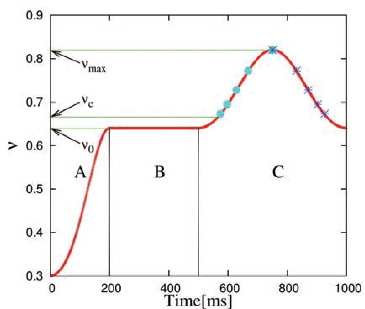
Evolution of volume fraction as a function of time. Region A represents the initial isotropic compression up to the initial volume fraction v₀. B represents relaxation of the system and C represents the subsequent isotropic compression up to v_max = 0.820 and then decompression. Cyan dots represent some of the initial configurations, at different v_i, during the loading cycle, and blue stars during the unloading cycle, both of which can be chosen for further study.

A general schematic representation of the procedure for implementing the isotropic and other deformation tests is shown in Fig. 2.

Fig. 2

Generic schematic representation of the procedure for implementing isotropic, uniaxial and deviatoric deformation element tests. The isotropic preparation stage is represented by the dashed box. The corresponding plots (not to scale) for the deviatoric strain against volumetric strain are shown below the respective modes. The solid square boxes in the flowchart represent the actual tests. The blue circles indicate the start of the preparation; the red triangles represent its end, i.e. the start of the test, while the green diamonds show the end of the respective test.

The compressed and relaxed configurations can now be used for other non-volume-conserving and/or stress-controlled modes (e.g. biaxial, triaxial and isobaric). One only has to use them as initial configurations and then decide which deformation mode to use, as shown in the figure under “other deformations”. The corresponding schematic plots of deviatoric strain ϵ_dev as a function of volumetric strain ϵ_v are shown below the respective modes.

3.2 Uniaxial

Uniaxial compression is one of the element tests that can be initiated at the end of the “preparation”, after sufficient relaxation indicated by the drop in potential energy to almost zero. The uniaxial compression mode in the triaxial box is achieved by a prescribed strain path in the z-direction, see Eq. (2), while the other boundaries x and y are non-mobile. During loading (compression), the volume fraction is increased as for isotropic compression from v₀ = 0.640 to a maximum volume fraction of v_max = 0.820 (as shown in region C of Fig. 1), and reverses back to the original volume fraction v₀ during unloading. Uniaxial compression is defined by the strain-rate tensor   

$$\dot{\mathbf{E}}={\dot{ϵ}}_{\text{u}}\hspace{0.17em}\left(\begin{array}{ccc}0& 0& 0\\ 0& 0& 0\\ 0& 0& -1\end{array}\right),$$

where ${\dot{ϵ}}_{\text{u}}$ is the strain-rate (compression > 0 and decompression/tension < 0) amplitude applied in the uniaxial mode. The negative sign (convention) of the component Ė_zz corresponds to a reduction of length, so that tensile deformation is positive. Even though the strain is imposed only on the mobile “wall” in the z-direction, which leads to an increase of compressive stress on this wall during compression, the non-mobile walls also experience some stress increase due to the “push-back” stress transfer and rearrangement of the particles during loading, as discussed in more detail in the following sections. This is in agreement with theoretical expectations for materials with non-zero Poisson’s ratio (Spencer, 1980). However, the stress on the passive walls is typically smaller than that of the mobile, active wall, as consistent with findings from laboratory element tests using the biaxial tester (Morgeneyer and Schwedes, 2003; Zetzener and Schwedes, 1998) or the so-called λ –meter.

3.3 Deviatoric

The preparation procedure as described in section 3.1 provides different initial configurations with volume fractions, v_i. For the deviatoric deformation element test, unless stated otherwise, the configurations are from the unloading part (represented by blue stars in Fig. 1), to test the dependence of quantities of interest on the volume fraction during volume-conserving deviatoric (pure shear) deformations. The unloading branch is more reliable since it is much less sensitive to the protocol and rate of deformation during preparation (Göncü et al., 2010, Kumar et al., 2012b). Two different ways of deforming the system deviatorically with conserved volume are used here. The deviatoric mode D2 has the strain-rate tensor   

$$\dot{\mathbf{E}}={\dot{ϵ}}_{\text{D}2}\hspace{0.17em}\left(\begin{array}{ccc}1& 0& 0\\ 0& 0& 0\\ 0& 0& -1\end{array}\right),$$

where ${\dot{ϵ}}_{\text{D2}}$ is the strain-rate (compression in z-direction > 0) amplitude applied to the walls. We use the nomenclature D2 since two walls are moving while the third wall is stationary. The deviatoric mode D3 has the strain-rate tensor   

$$\dot{\mathbf{E}}={\dot{ϵ}}_{\text{D}3}\hspace{0.17em}\left(\begin{array}{ccc}1/2& 0& 0\\ 0& 1/2& 0\\ 0& 0& -1\end{array}\right),$$

where ${\dot{ϵ}}_{\text{D3}}$ is the strain-rate (> 0 for compression in z-direction) amplitude applied. In this case, D3 signifies that all three walls are moving, with one wall twice as much (in the opposite direction) as the other two such that volume is conserved during deformation.

Note that the D3 mode is uniquely similar in “shape” to the uniaxial mode¹, see Table 1, since in both cases two walls are controlled similarly. Mode D2 is different in this respect and thus resembles more an independent mode (pure shear), so that unless differently stated, we plot by default the D2 results rather than the D3 ones (see section 2). The mode D2 with shape factor (as defined in Table 1) ζ = 0 is on the one hand a plane strain deformation, and on the other hand allows for simulation of the biaxial experiment (with two walls static while four walls are moving, see Morgeneyer and Schwedes, 2003; Zetzener and Schwedes, 1998).

Table 1 Summary of the deformation modes and the deviatoric strain rates ${\dot{ϵ}}_{\text{dev}}$, as well as shape factors, ζ, and Lode angles, α, (Thornton and Zhang, 2010) for the different modes in the respective tensor eigensystem, with sorted eigenvalues ${ϵ}_{\text{d}}^{\left(1\right)}\ge {ϵ}_{\text{d}}^{\left(2\right)}$, defined in section 4.2.1

Mode	Strain-rate tensor (main diagonal, sorted)	Deviatoric strain rate (magnitude)	$\zeta ={ϵ}_{\text{d}}^{\left(2\right)}/{ϵ}_{\text{d}}^{\left(1\right)}$	Lode angle $\alpha ={\text{tan}}^{-1}\hspace{0.17em}\left[\frac{1}{\sqrt{3}}\left(1+2\zeta \right)\right]$
ISO (isotropic compression)	${\dot{ϵ}}_{\text{v}}$ (−1, −1, −1)	${\dot{ϵ}}_{\text{dev}}=0$	n.a.	n.a.
UNI (uniaxial compression)	${\dot{ϵ}}_{\text{u}}$ (0, 0, −1)	${\dot{ϵ}}_{\text{dev}}={\dot{ϵ}}_{\text{u}}={\dot{ϵ}}_{\text{zz}}$	1	60°
D2 (pure shear – plane strain)	${\dot{ϵ}}_{\text{D2}}$ (1, 0, −1)	${\dot{ϵ}}_{\text{dev}}=\sqrt{3}{\dot{ϵ}}_{\text{D}2}$	0	30°
D3 (axisymmetric compression)	${\dot{ϵ}}_{\text{D}3}$ (1/2, 1/2, −1)	${\dot{ϵ}}_{\text{dev}}=\text{(3/2)}{\dot{ϵ}}_{\text{D}3}$	1	60°

1  The more general, objective definition of deviatoric deformations uses the orientation of the stresses (eigen-directions) in the deviatoric plane from the eigenvalues, as explored elsewhere (Kumar et al., 2012a; Thornton and Zhang, 2006, 2010), since this is beyond the scope of this study.

4. Averaged Quantities

In this section, we present the general definitions of averaged microscopic and macroscopic quantities. The latter are quantities that are readily accessible from laboratory experiments, whereas the former are often impossible to measure in experiments but are easily available from discrete element simulations.

4.1 Averaged microscopic quantities

Here, we define microscopic parameters including the coordination number, the fraction of rattlers, and the ratio of the kinetic and potential energy.

4.1.1 Coordination number and rattlers

In order to link the macroscopic load carried by the sample with the microscopic contact network, all particles that do not contribute to the force network – particles with exactly zero contacts – are excluded. In addition to these “rattlers” with zero contacts, there may be a few particles with a finite number of contacts for a short time which also do not contribute to the mechanical stability of the packing. These particles are called dynamic rattlers (Göncü et al., 2010), since their contacts are transient: The repulsive contact forces will push them away from the mechanically stable backbone. Frictionless particles with less than 4 contacts are thus rattlers, since they are mechanically unstable and hence do not contribute to the contact network. In this work, since tangential forces are neglected, rattlers can be identified by just counting their number of contacts. This leads to the following abbreviations and definitions for the coordination number (i.e. the average number of contacts per particle) and fraction of rattlers, which must be reconsidered for systems with tangential forces or torques:

N:

Total number of particles

N₄:= N_{c≥ = 4}:

Number of particles with at least 4 contacts

M:

Total number of contacts

M₄:= M_{c≥ = 4}:

Number of contacts of particles with at least 4 contacts

${\varphi }_r:=\frac{N-N_4}{N}$:

(Number) fraction of rattlers

$C^r:=\frac{M}{N}$:

Coordination number (simple definition)

$C=C^m:=\frac{M_4}{N}$:

Coordination number (modified definition)

$C^{*}:=\frac{M_4}{N_4}=\frac{C}{1-{\varphi }_r}$:

Corrected coordination number

$v:=\frac{1}{V}{\sum }_{p\in N}{V}^p$:

Volume fraction of the particles, with V ^p as particle volume.

Some simulation results for the coordination numbers and the fraction of rattlers will be presented below in subsection 5.1.

4.1.2 Energy ratio and quasi-static criterion

Above the jamming volume fraction v_c, in mechanically stable static situations, there exist permanent contacts between particles; hence the potential energy (which is also an indicator of the overlap between particles) is considerably larger than the kinetic energy (which has to be seen as a perturbation).

The ratio of kinetic energy and potential energy is shown in Fig. 3 for isotropic compression from v₀ = 0.640 to v_max = 0.820 and back. The first simulation, represented by the solid red line, was run for a simulation time T = 5000 [μs] and the second (much slower) simulation, represented by the green dashed line was run for T = 50000 [μs]. For these simulations, the maximum strain rates are ${\dot{ϵ}}_{zz}^{\text{max}}=138\hspace{0.17em}\left[{\text{s}}^{-1}\right]$ and 13.8 [s⁻¹], respectively. During compression with increasing volume fraction, the energy ratio generally decreases and slower deformation by a factor of 10 leads to more than 100 times smaller energy ratios with stronger fluctuations. Most sharp increases of the energy ratio resemble reorganization events of several particles and are followed by an exponentially fast decrease (data not shown). The decrease is controlled by the interaction and dissipation timescales and not by the shear rate; in other words the timescale of energy dissipation t_d ≈ 10⁻⁵ [s] is considerably smaller than the simulation timescale t_s ≈ 7.2 10⁻³ [s] or 7.2 10⁻² [s], so that kinetic energy can be well relaxed before a considerable rearrangement of particles takes place; due only to the scaling of τ = t/T, the decrease appears to be faster for the slower deformation. Explicitly, the rate of decay depends on material parameters only and is of the order of 1/t_e, however, it becomes larger the closer to jamming one gets. The large initial ratio of kinetic to potential energy (E_k/E_p > 1) indicates that the system is in the unjammed regime, whereas after some compression it enters the quasi-static regime with much smaller energy ratios (Thornton and Anthony, 1998). In this way, dynamic effects are minimized and the system is as close as feasible to the quasi-static state. For many situations, it was tested that a slower deformation did not lead to large, considerably different results. For the majority of the data presented, we have (E_k/E_p ≤ 10⁻³). Lower energy ratios can be obtained by performing simulations at even slower rates, but the settings used are a compromise between computing time and reasonably slow deformations.

Fig. 3

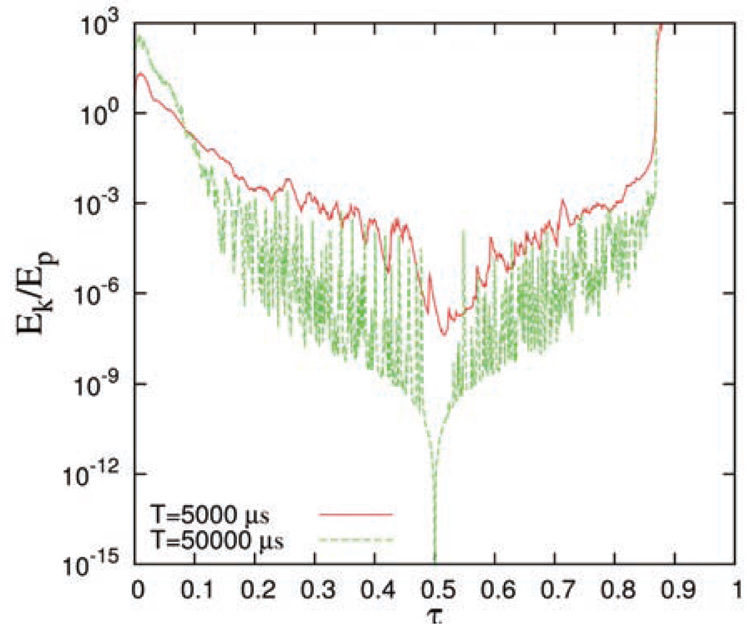
Comparison of the ratio of kinetic and potential energy in scaled time (τ = t/T) for two simulations, with different period of one compression-decompression cycle T, as given in the inset.

4.2 Averaged macroscopic quantities

Now the focus is on defining averaged macroscopic tensorial quantities – including strain, stress and fabric (structure) tensors – that reveal interesting bulk features and provide information about the state of the packing due to its deformation.

4.2.1 Strain

For any deformation, the isotropic part of the infinitesimal strain tensor ϵ_v is defined as:   

$${ϵ}_{\text{v}}={\dot{ϵ}}_{\text{v}}\text{dt}=\frac{{ϵ}_{xx}+{ϵ}_{yy}+{ϵ}_{zz}}{3}+\frac{1}{3}\text{tr}\left(\mathbf{E}\right)=\frac{1}{3}\text{tr}\left(\dot{\mathbf{E}}\right)\text{dt},$$(3)

where ${\stackrel{}{ϵ}}_{\text{αα}}$ = ${\dot{ϵ}}_{\text{αα}}$ dt with αα = xx, yy or zz are the diagonal elements of the strain tensor E in the Cartesian x, y, z reference system. The trace integral of $3{ϵ}_{\text{v}}$, denoted by ε_v is the true or logarithmic strain, i.e. the volume change of the system relative to the initial reference volume V₀ (Göncü et al., 2010).

Several definitions are available in literature (Imole et al., 2011; Thornton and Zhang, 2006, 2010; Zhao and Evans, 2011) to define the deviatoric magnitude of the strain. For the sake of simplicity, we use the following definition of the deviatoric strain to account for all active and inactive directions in a triaxial experiment, regardless of the deformation mode,   

$${ϵ}_{\text{dev}}=\sqrt{\frac{{\left({ϵ}_{xx}-{ϵ}_{yy}\right)}^2+{\left({ϵ}_{yy}-{ϵ}_{zz}\right)}^2+{\left({ϵ}_{zz}-{ϵ}_{xx}\right)}^2}{2}},$$(4)

Since, for our triaxial box, for all modes, the Cartesian coordinates resemble the fixed eigensystem, sorting the eigenvalues according to magnitude ${ϵ}_d^{\left(1\right)}\ge {ϵ}_d^{\left(2\right)}\ge {ϵ}_d^{\left(3\right)}$ leaves the eigenvalue ${ϵ}_d^{\left(1\right)}$ as the maximal tensile eigenvalue, with corresponding eigendirection, and ϵ_dev ≥ 0 as the magnitude of the deviatoric strain². The quantitative description of the tensor is completed by either its third invariant, the Lode angle α (Thornton and Zhang, 2010) or, equivalently, by the shape factor ζ, as given in Table 1. Note that the values for ζ are during uniaxial loading where compression is performed in the z-direction. The sorting will lead to different values, ζ = −1/2, when the strain is reversed for both UNI and D3 modes.

2  The objective definition of the deviatoric strain defines it in terms of the eigenvalues ${ϵ}_{\text{d}}^{\left(1\right)}$, ${ϵ}_{\text{d}}^{\left(2\right)}$ and ${ϵ}_{\text{d}}^{\left(3\right)}$, of the (deviatoric) strain tensor. However, since the global strain is given by the wall motion and the eigensystem stays practically unchanged during the deformation, the two definitions are equivalent for triaxial element tests.

4.2.2 Stress

From the simulations, one can determine the stress tensor (compressive stress is positive as convention) components:   

$${\sigma }_{\alpha \beta }=\frac{1}{V}\left(\sum _{p\in V}{m}^p{v}_{\alpha }^p{v}_{\beta }^p-\sum _{c\in V}{f}_{\alpha }^c{l}_{\beta }^c\right),$$(5)

with particle p, mass m ^p, velocity v ^p, contact c, force f ^c and branch vector l ^c, while Greek letters represent components x, y, and z (Luding, 2008a,b). The first sum is the kinetic energy tensor and the second involves the contact-force dyadic product with the branch vector. Averaging, smoothing or coarse graining (Weinhart et al., 2012) in the vicinity of the averaging volume, V, weighted according to the vicinity, is not applied in this study, since averages are taken over the total volume. Since the data in this study are quasi-static, the first sum can mostly be neglected.

The average isotropic stress (i.e. the hydrostatic pressure) is defined as:   

$$P=\frac{{\sigma }_{xx}+{\sigma }_{yy}+{\sigma }_{zz}}{3}=\frac{1}{3}\text{tr}\left(\mathbf{\sigma }\right),$$(6)

where σ_xx, σ_yy and σ_zz are the diagonal elements of the stress tensor σ in the x, y, and z box reference system and tr(σ) is its trace. The non-dimensional pressure (Göncü et al., 2010) is defined as:   

$$p=\frac{2⟨r⟩}{3k}\text{tr}\left(\mathbf{\sigma }\right),$$(7)

where ⟨r⟩ is the mean radius of the spheres and k is the contact stiffness defined in section 2. We define the deviatoric magnitude of stress (similar to Eq. (4) for the deviatoric strain) as:   

$${\sigma }_{\text{dev}}=\sqrt{\frac{{\left({\sigma }_{xx}-{\sigma }_{yy}\right)}^2+{\left({\sigma }_{yy}-{\sigma }_{zz}\right)}^2+{\left({\sigma }_{zz}-{\sigma }_{xx}\right)}^2}{2}},$$(8)

which is always positive by definition. The direction of the deviatoric stress is carried by its eigen-directions (in the present case coincident with the Cartesian reference system), where stress eigenvalues are sorted like strain eigenvalues, possibly with a different sign convention, according to their magnitude. Eqs. (4) and (8) can easily be generalized to account for shear reversal using a sign taken from the orientation of the corresponding eigenvectors and eigenvalues, or from the stress shape factor, however, this will not be detailed here for the sake of brevity.

It is noteworthy to add that the definitions of the deviatoric stress and strain tensors are proportional to the second invariants of these tensors, e.g. for stress: $J_2=\left(1/\sqrt{3}\right){\sigma }_{\text{dev}}$, which makes our definition identical to the von Mises criterion (Fredlund, 1979; Hayhurst, 1972; Thornton and Zhang, 2006, 2010)³.

3  Different factors in the denominator of Eqs. (4) and (8) have been proposed in literature (Imole et al., 2011; Zhao and Evans, 2011) but they only result in a change in the maximum deviatoric value obtained. For consistency, we use the same factor $\sqrt{1/2}$ for deviatoric stress and strain and a similar definition for the deviatoric fabric, see the next subsection.

4.2.3 Fabric (structure) tensor

Besides the stress of a static packing of powders and grains, the next most important quantity of interest is the fabric/structure tensor. For disordered media, the concept of the fabric tensor naturally occurs when the system consists of an elastic network or a packing of discrete particles. The expression for the components of the fabric tensor is:   

$$F_{\alpha \beta }=\frac{1}{V}\sum _{p\in V}{V}^p\sum _{\text{c}=1}^N{n}_{\alpha }^{\text{c}}{n}_{\beta }^{\text{c}},$$(9)

where V ^p is the particle volume which lies inside the averaging volume V and n^c is the normal unity vector pointing from the center of particle p to contact c. F_αβ are thus the components of a symmetric rank- two 3×3 tensor, such as the stress tensor. The isotropic fabric F_v = tr(F) quantifies the contact number density as studied by Göncü et al., 2010. We assume that the structural anisotropy in the system is quantified (completely) by the anisotropy of fabric, i.e. the deviatoric fabric. To quantify it, we define a scalar similar to Eqs. (4) and (8) as:   

$$F_{\text{dev}}=\sqrt{\frac{{\left(F_{xx}-F_{yy}\right)}^2+{\left(F_{yy}-F_{zz}\right)}^2+{\left(F_{zz}-F_{xx}\right)}^2}{2}},$$(10)

where F_xx, F_yy and F_zz are the three diagonal components of the fabric tensor. The fabric tensor practically has only diagonal components with non-diagonal elements very close to zero, so that its eigensystem is close to the Cartesian reference system, as confirmed by eigenvalues analysis. Also for the fabric, a shape factor completes the picture.

4.2.4 Conclusion

Three macroscopic rank-two tensors were defined and will be related to microscopic quantities and each other in the following. The orientations of all the tensor eigenvectors show a tiny non-co-linearity of stress, strain and fabric, which we neglect in the next sections, since we attribute it to natural statistical fluctuations and consider a unique fixed eigensystem coincident with the Cartesian reference system for all our deformation modes. The shape factor, as defined for strain, can also be analyzed for stress and fabric, but this will be shown elsewhere.

5. Evolution of Micro-Quantities

In this section, we discuss the evolution of the microscopic quantities studied – including coordination number and fraction of rattlers – as a function of volume fraction and deviatoric strain, respectively, and compare these results for the different deformation modes.

5.1 Coordination number and rattlers

It has been observed by Göncü et al., 2010, that under isotropic deformation, the corrected coordination number C^* follows the power law   

$$C^{*}\left(v\right)=C_0+C_1{\left(\frac{v}{v_c}-1\right)}^{\alpha },$$(11)

where C₀ = 6 is the isostatic value of C^* in the frictionless case. For the uniaxial unloading simulations, we obtain C₁ ≈ 8.370, α ≈ 0.5998 and $v_c^{\text{UNI}}\approx 0.6625$ as best-fit parameters.

In Fig. 4, the evolution of the simple, corrected and modified coordination numbers is compared as a function of the volume fraction during uniaxial deformation (during one loading and unloading cycle). The contribution to the coordination number originating from particles with C = 1, 2 or 3 is small – as compared to those with C = 0 – since C^r and C^m are very similar, but always smaller than C^* due to the fraction of rattlers, as discussed below. The number of contacts per particle grows with increasing compression to a value of C^* = 9.5 at maximum compression. During decompression, the contacts begin to open and the coordination number decreases and approaches the theoretical value C₀ = 6 at the critical jamming volume fraction⁴ after uniaxial decompression $v_c^{\text{UNI}}\approx 0.662$. Note that the $v_c^{\text{UNI}}$ value is smaller than $v_c^{\text{ISO}}\approx 0.665$ reached after purely isotropic over-compression to the same maximal volume fraction. The coordination numbers are typically slightly larger in the loading branch than in the unloading branch, due to the previous over-compression.

Fig. 4

Comparison between coordination numbers using the simple (‘+’, blue), modified (‘⟐’, green) and corrected (‘▿’, red) definitions. Data are from a uniaxial compression-decompression simulation starting from v₀ = 0.64 < v_c ≈ 0.6625. The solid black line represents Eq. (11) with parameters given in the text very similar to those measured in Göncü et al., 2010, see Table 2. The compression and decompression branches are indicated by arrows pointing right and left, respectively.

In Fig. 5, we plot the corrected coordination number for deformation mode D2 as a function of the deviatoric strain for five different volume fractions. Two sets of data are presented for each volume fraction starting from different initial configurations, either from the loading or the unloading branch of the isotropic preparation simulation (cyan dots and blue stars in Fig. 1). Given initial states with volume fractions above the jamming volume fraction, and due to the volume-conserving D2 mode, the value of the coordination number remains practically constant. It is only for the lowest volume fractions close to jamming, that a slight increase (decrease) in C^* can be seen for the initial states chosen from the unloading (loading) branch of the preparation step.

Fig. 5

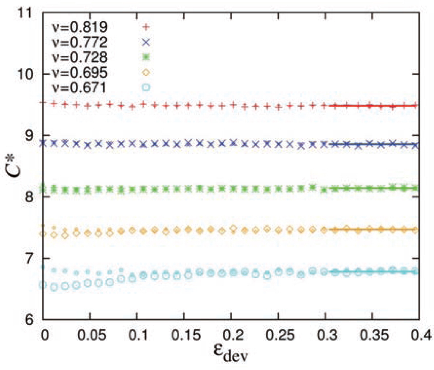
Evolution of coordination numbers with deviatoric strain for the D2 mode. Smaller symbols represent data with initial configuration from the loading branch of an isotropic simulation, while the larger symbols start from an initial configuration with the same volume fraction, but from the isotropic unloading branch. The horizontal line at the large strain of the dataset indicates an average after saturation at steady state.

However, both reach similar steady-state values after large strain, as indicated by the solid lines. Hence, for further analysis and unless otherwise stated, we will only present the steady-state values of micro- and macro-quantities from deviatoric modes D2 and D3.

The rearrangement of the particles during shear thus does not lead to the creation (or destruction) of many contacts – on average. There is no evidence of the change of average contacts after 10 – 15 percent of strain. However, close to jamming, a clear dependence of C^* on the initial state exists, which vanishes in steady state when one gets saturated values in micro- and macro-quantities after large enough strain. For the same volume fraction, we evidence a range of $C_{\text{oc}}^{*}\le C_{\text{s}}^{*}\approx C_{\text{ic}}^{*}$, where the subscripts refer to over-compressed, steady, and initially compressed states, respectively. The coordination number, or alternatively the contact number density, as related to the trace of the fabric tensor (Göncü et al., 2010), is thus a control parameter closely linked to the volume fraction that contains more information about the structure than v itself (above the jamming volume fraction), see Magnanimo et al., 2008 and references therein.

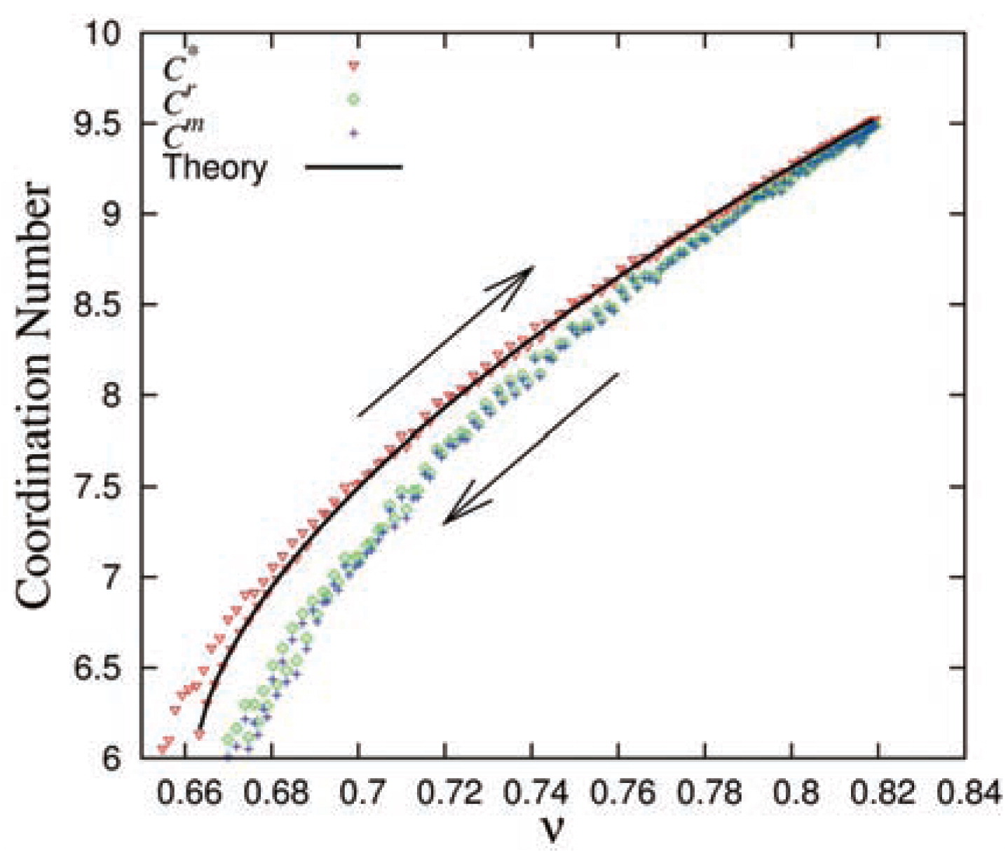
In Fig. 6, the corrected coordination number is shown as a function of volume fraction for the purely isotropic and for the uniaxial unloading data as well as for the large strain deviatoric deformation data-sets. Different symbols show the values of C^* for the different deformation modes for various volume fractions. Interestingly, the power law for the coordination number derived from isotropic data describes well also the uniaxial and deviatoric datasets, with coefficients given in Table 2. This suggests that (for the cases considered, when particles are frictionless) the coordination number is almost independent of the deviatoric strain in steady state, and the limit values can be approximated by Eq. (11) as proposed for simple isotropic deformation. The distinction between the modes at the small (isotropic) strain region is shown zoomed in the inset of Fig. 6. The mixed mode (uniaxial) is bordered on both sides by the pure modes, namely isotropic and deviatoric (D2 and D3 cannot be distinguished), indicating that the two pure modes are limit states or extrema for C^*. Alternatively, the range in C^* values can be seen as caused by a range in v_c, with $v_c^{\text{ISO}}>v_c^{\text{UNI}}>v_c^{\text{DEV}}$, which represent the maximal jamming volume fraction after previous (isotropic, strong) over-compression, the intermediate jamming volume fraction after (mixed mode) deformation, and the minimal jamming volume fraction after large deviatoric strain, respectively, with $v_c^{\text{ISO}}\approx 0.6646$ and $v_c^{\text{DEV}}\approx 0.6602$.

Fig. 6

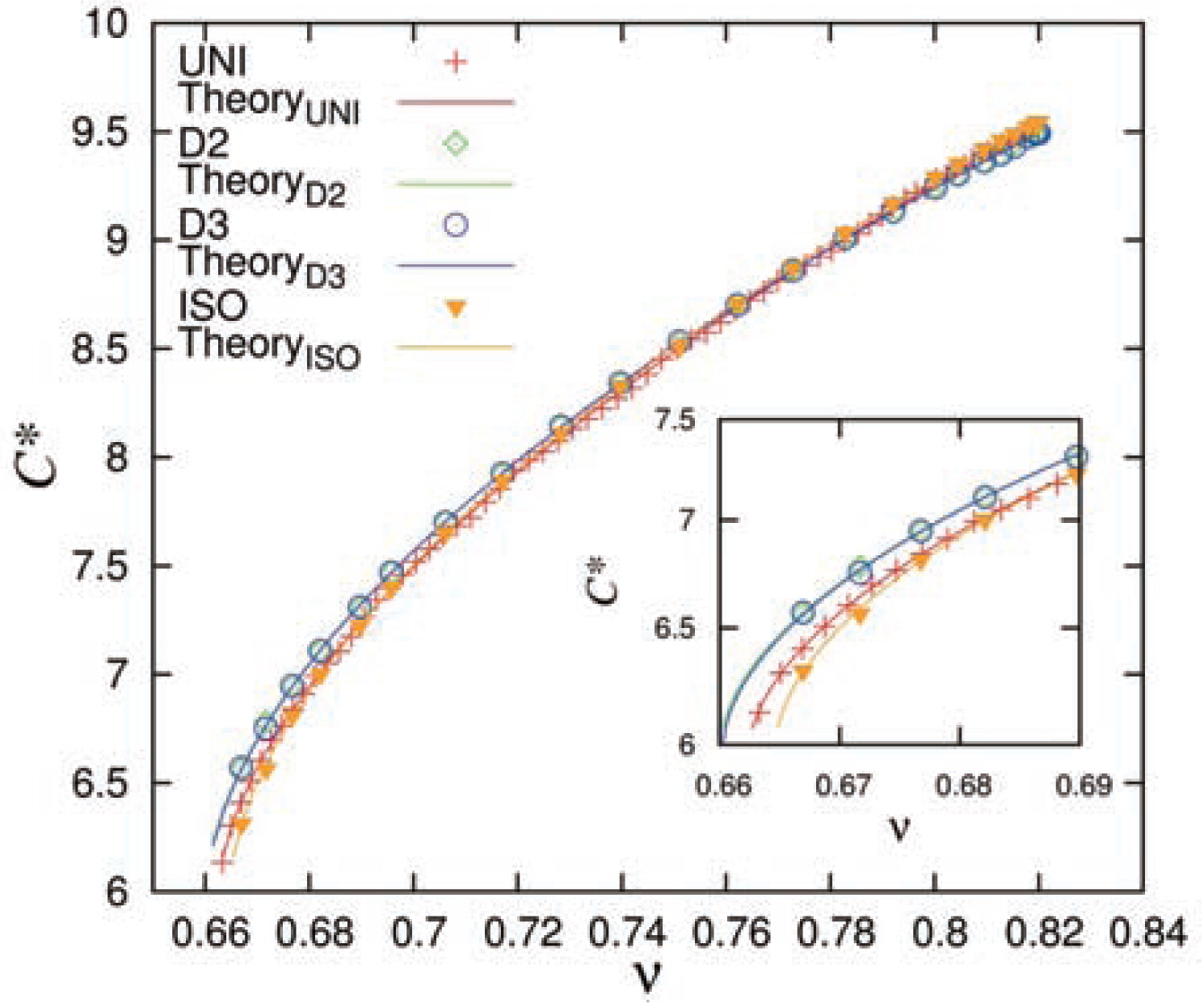
Evolution of the corrected coordination number as a function of volume fraction during unloading for all modes. The symbols represent the respective simulation data while the solid lines represent the analytical equation according to Eq. (11) with the respective values of C₀, C₁, α and v_c shown in Table 2. The inset shows the corrected coordination number at low volume fractions close to jamming.

Table 2 Fit parameters for the analytical predictions of coordination number, fraction of rattlers, and pressure in Eq. (11), with C₀ = 6 and Eqs. (12) and (15), respectively. v_c is used from the fits of C^* to fit ϕ_r for the different deformation modes. The first rows of isotropic data ISOG are from Göncü et al., 2010, for various polydispersities and also during unloading, but for different over-compression density.

C*	C1	α	vc
ISOG	8.0 ± 0.5	0.58 ± 0.05	0.66 ± 0.01
ISO	8.2720	0.5814	0.6646
UNI	8.3700	0.5998	0.6625
D2	7.9219	0.5769	0.6601
D3	7.9289	0.5764	0.6603

ϕr	ϕc	ϕv
ISOG	0.13 ± 0.03	15 ± 2
ISO	0.1216	15.8950
UNI	0.1507	15.6835
D2	0.1363	15.0010
D3	0.1327	14.6813

p*	p0	γp	vc
ISOG	0.04180	0.11000	0.6660
ISO	0.04172	0.06228	0.6649
UNI	0.04006	0.03270	0.6619
D2	0.03886	0.03219	0.6581
D3	0.03899	0.02819	0.6583

In other words, deviatoric deformations reduce the jamming volume fraction of the packing, i.e. can disturb and dilate a dense (over-compressed) packing so that it becomes less efficiently packed. This is opposite to isotropic over-compression, where after unloading, the jamming volume fraction is higher, i.e. the system is more efficiently packed/structured. This behavior is qualitatively expected for frictional particles, however, this is to our knowledge the first time that this small but systematic range in the jamming volume fractions is reported for frictionless packings – where the most relevant and only mechanism is structural reorganization, as will be discussed further in section 6.1.1.

As a related interesting microscopic quantity, we recall the analytical expression for the fraction of rattlers proposed by Göncü et al., 2010:   

$${\varphi }_r\left(v\right)={\varphi }_c\hspace{0.17em}\text{exp}\left[-{\varphi }_v\left(\frac{v}{v_c}-1\right)\right],$$(12)

where the fit parameters for the different deformation modes are given in Table 2, and v_c ≈ 0.6646 is obtained from extrapolation of C^* to the isostatic coordination number C₀ = 6. In Fig. 7, the evolution of the fraction of rattlers is plotted as a function of volume fraction for both isotropic and uniaxial unloading as well as for steady-state deviatoric mode simulations. We then compare these with the prediction/ fit (solid lines) from the exponential decay equation, Eq. (12). Interestingly, in contrast to the coordination number, the fraction of rattlers displays stronger differences at the highest volume fraction (v = 0.82 in Fig. 7), and it is lower during isotropic unloading as compared to the steady-state deviatoric mode situations, and somewhat higher during uniaxial unloading. The difference between the modes is small close to jamming with largest ϕ_r for the UNI mode. For uniaxial simulations, at the end of unloading close to $v_c^{\text{UNI}}$, a considerable fraction (almost 20 percent) of the total number of particles are rattlers that do not contribute to the stability of the network. For higher volume fractions, a strong exponential decay is evidenced⁵.

Fig. 7

Evolution of the fraction of rattlers as a function of volume fraction during unloading for all modes. The symbols represent the respective simulation data. The solid lines are the analytical fits of Eq. (12) for each mode with the values of fit parameters ϕ_c and ϕ_v for each mode shown in Table 2. The arrow indicates the unloading direction.

To better understand the peculiar behavior of the jamming volume fraction under the different modes of deformation, some macroscopic quantities are studied next.

4  The value, C₀ = 6, is expected since it is the isostatic limit for frictionless systems in three dimensions (Göncü et al., 2010; Maxwell, 1864), for which the number of constraints (contacts) is twice the number of degrees of freedom (dimension) – in average, per particle – so that the number of unknown forces matches exactly the number of equations. (C₀ is different from the minimal number of contacts needed for a single mechanically stable frictionless sphere $C_{\text{min}}^p$ in 3D).

5  The sharp jump observed in Göncü et al., 2010 at the jamming transition during unloading is not seen here because we keep the system above the jammed state. Interestingly, the simulation data for the uniaxial and deviatoric mode all collapse close to the (isotropic) exponential prediction.

6. Evolution of Macro-Quantities

In the following, we discuss the evolution of the macroscopic tensors, stress and fabric, as defined in section 4.2. For clarity, we split them into isotropic and deviatoric parts in subsections 6.1 and 6.2, respectively.

6.1 Evolution of macro-quantities: isotropic

6.1.1 Isotropic pressure

In this section, the relation between pressure and volume fraction is studied. First, we consider the contact overlap/deformation δ_c, since the force is directly related to it and stress is proportional to the force. The infinitesimal change d⟨Δ⟩_c = 3Zϵ_v of the normalized average overlap Δ_c = δ_c/⟨r⟩, can be related to the volumetric strain under the simplifying assumption of uniform, homogeneous deformation in the packing. As defined in subsection 4.2.1, ϵ_v = ϵ_ii/3 is the average of the diagonal elements of the infinitesimal strain tensor, and Z ≈ 0.425 is a proportionality constant that depends on the size distribution and can be readily obtained from the average overlap and volume fraction (data not shown), see Eq. (13). The integral of 3ϵ_v denoted by ε_v is the true or logarithmic volume change of the system relative to the reference volume V_ref. This is chosen without loss of generality at the critical jamming volume fraction v_ref = v_c, so that the normalized average overlap is (Göncü et al., 2010):   

$${⟨\mathrm{\Delta }⟩}_c=-3Z\hspace{0.17em}{\int }_{V_0}^V\hspace{0.17em}{ϵ}_{\text{v}}=-Z{\epsilon }_{\text{v}}=Z\hspace{0.17em}\text{ln}\hspace{0.17em}\left(\frac{v}{v_c}\right).$$(13)

As in Eq. (7), see Refs. Göncü et al., 2010; Shaebani et al., 2012 for details, the non-dimensional pressure is:   

$$p=\frac{2⟨r⟩}{3k}\text{tr}\left(\mathbf{\sigma }\right)=p_0\frac{vC}{v_c}\left(-{\epsilon }_{\text{v}}\right)\left[1-{\gamma }_p\left(-{\epsilon }_{\text{v}}\right)\right],$$(14)

and the scaled pressure is:   

$$p^{*}=\frac{p{v}_c}{vC}=p_0\left(-{\epsilon }_{\text{v}}\right)\left[1-{\gamma }_p\left(-{\epsilon }_{\text{v}}\right)\right],$$(15)

where p₀ ≈ 0.040, γ_p ≈ 0.033, and the critical volume fraction v_c ≈ 0.6625 are fit parameters to the pressure law for uniaxial unloading. Combining the quasi-static part of Eq. (5) with (14) leads to the proportionality relation p ∝ vC⟨Δ⟩_c, which makes p a measure for the average overlap relative to the average particle diameter. On the other hand p^* in Eq. (15) scales various different pressures p for different deformation modes to their respective reference jamming volume fractions and is linear for small ε_v.

Note that the critical volume fraction v_c = 0.6625, as obtained from extrapolation of C^* to the isostatic coordination number C₀ = 6, is very close to that obtained from Eq. (14). When fitting all modes with pressure, one confirms again that $v_c^{\text{UNI}}$ falls in between the limits of the pure modes $v_c^{\text{ISO}}$ and $v_c^{\text{DEV}}$ (with values consistent within each mode) as summarized in Table 2.

In Fig. 8, we plot the total (non-dimensional) pressure p as a function of the deviatoric strain for different volume fractions in the deformation mode D2. Above the jamming volume fraction, the value of the pressure stays practically constant with increasing shear strain. A slight increase in p can be seen for the lowest volume fractions when the initial states are chosen from the unloading branch of isotropic modes, whereas a slight decrease in p is observed for initial states chosen from the loading branch. Independently of the initial configuration, the pressure reaches a unique steady state at large strain, similarly to what is observed for the coordination number in Fig. 6.

Fig. 8

Evolution of (non-dimensional) pressure, Eq. (7), with deviatoric strain for the D2 deformation mode, at different initial volume fractions v_i. Small and large symbols represent simulations starting with initial isotropic configurations from the loading and unloading branch, respectively. The horizontal line at the large strain of the dataset indicates an average value of the pressure after saturation at steady state.

In Fig. 9, the total pressure is plotted against volume fraction for isotropic, uniaxial and deviatoric (D2 and D3) modes, with data obtained from the unloading branch in the first two cases and after large deviatoric strain for the deviatoric modes (see Fig. 8). For these three modes, at large v, the simulation data collapse on a unique curve with non-linear behavior. Due to the linear contact model, this feature can be directly related to the contact number density, i.e. the isotropic fabric, which quantifies the isotropic, direction-independent changes of structure due to rearrangements and closing/opening of contacts. When approaching the jamming transition, the pressure values diverge slightly (inset of Fig. 9) due to the difference in the critical volume fractions $v_c^{\text{DEV}}<v_c^{\text{UNI}}<v_c^{\text{ISO}}$.

Fig. 9

Total (non-dimensional) pressure, Eq. (14), plotted as a function of volume fraction for the uni-axial and isotropic datasets during unloading, and for the D2/D3 deviatoric modes after large strain. The solid lines are the analytical fits of Eq. (14) for each mode, with parameters p₀, γ_p and v_c shown in Table 2.

In Fig. 10, we plot the scaled pressure defined in Eq. (15) against the volumetric strain from the same data as in Fig. 9. The three datasets almost collapse for small strain. For increasing volume fractions (larger −ε_v), the scaled pressure in the isotropic mode is considerably larger than the uniaxial and deviatoric modes, where again the uniaxial data fall in between isotropic and deviatoric values. This resembles the behavior of C^* and is consistent with the fact that the uniaxial mode is a superposition of the purely isotropic and deviatoric deformation modes.

Fig. 10

The scaled pressure plotted against the (negative) volumetric strain for the same data as presented in Fig. 9. The solid lines are the predictions from Eq. (15) using the fits of p and C for each mode.

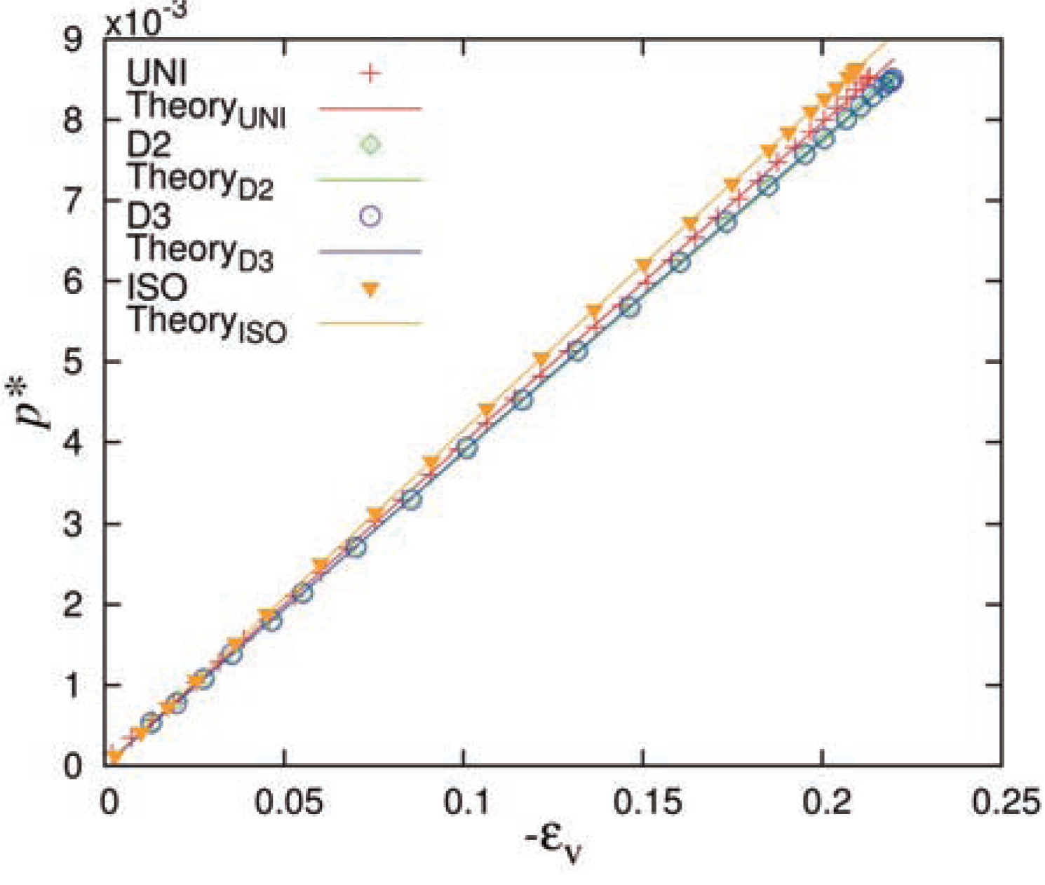
The dependence of pressure on isotropic strain can be interpreted in relation to the sample history. The deviatoric modes (D2 or D3) lead to dilatancy and thus to higher steady-state pressure, with low $v_c^{\text{DEV}}$; the isotropic mode is strictly compressive, with the lowest pressure after over-compression, during unloading and the highest $v_c^{\text{ISO}}$; finally, the uniaxial mode is a mixed mode and thus interpolates between the two other modes.

The apparent collapse of all scaled p^* data at small strain, with similar pre-factors p₀ ≈ 0.040 is interesting since, irrespective of the applied deformation mode – purely isotropic, uniaxial, and D2 or D3 deviatoric, it boils down to a linear relation between p^* and −ε_v with a small quadratic correction – different from the non-linear power laws proposed in previous studies, e.g. in Majmudar et al., 2007. The non-linearity due to 1 − v/v_c is hidden in vC, which is actually proportional to the isotropic fabric F_v.

6.1.2 Isotropic fabric

The random isotropic orientation of the contact directions in space was studied in detail in Refs. Göncü et al., 2010 and Shaebani et al., 2012, and is referred to as the contact number density with tr(F) = g₃vC, where g₃ is of order unity and depends only on the size distribution (for our case with w = 3, one has g₃ ≈ 1.22). Note that vC directly connects to the dimensionless pressure which, remarkably, hides the corrected coordination number and the fraction of rattlers in the relation C = (1 − ϕ_r)C^*, which fully determines tr(F).

6.2 Evolution of macro-quantities: deviatoric

In the following, we will show the evolution of the deviatoric stress ratio (which can be seen as a measure of stress anisotropy) and the structural anisotropy, both as a function of the deviatoric strain. In particular, we present the raw data from deviatoric and uniaxial simulations and their phenomenology. The D2 volume-conserving simulations are used to calibrate the constitutive model, as presented in Refs. Luding and Perdahcioğlu, 2011, Magnanimo and Luding, 2011 and described in section 7. We further use the fitting parameters inferred from deviatoric data to predict the evolution of stress and fabric during uni-axial deformation.

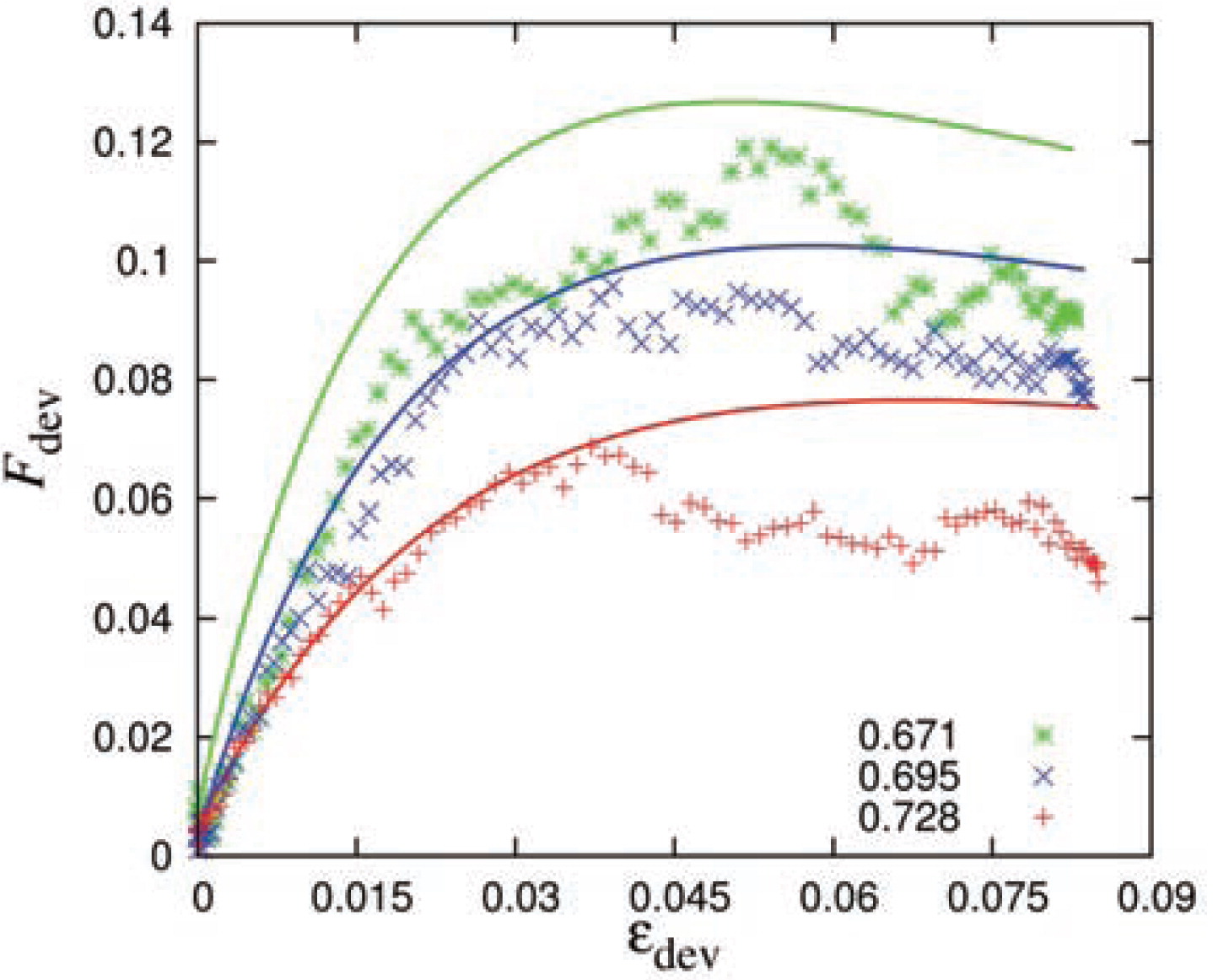
6.2.1 Deviatoric stress

The behavior of the deviatoric stress ratio, s_dev = σ_dev/P during deformation mode D2, is shown in Fig. 11 as a function of the deviatoric strain for various different volume fractions. The stress ratio initially grows with applied strain until an asymptote (the maximum stress anisotropy) is reached where it remains fairly constant. The asymptote $s_{\text{dev}}^{\text{max}}={\left({\sigma }_{\text{dev}}/P\right)}^{\text{max}}$ is referred to as the deviatoric steady state or the macroscopic friction, where s_dev represents the mobilized friction at each step along the loading path. For lower volume fractions, higher maximum s_dev are reached and the deviatoric stress ratio increases faster, meaning a higher G^oct/P ratio, where G^oct is the octahedral shear modulus as defined by Barreto and O’Sullivan, 2012. This is opposite to what is expected for the shear modulus G^oct itself, being proportional to the volume fraction. Interestingly, the stress response observed for mode D3 (not shown) follows a very similar path as for mode D2, resembling independency of the results with respect to the particular deviatoric path, as will be discussed in more detail in section 7.

Fig. 11

Deviatoric stress ratio (s_dev =σ_dev/P) plotted against deviatoric strain from the D2 deformation mode for initial volume fractions v_i during unloading, from which the simulations were performed, as given in the inset. The symbols (‘*’, ‘×’ and ‘+’) are the simulation data while the solid lines through them represent a fit to the data using Eq. (17).

We use the deviatoric simulations to fit the exponential relation proposed in Luding and Perdahcioğlu, 2011; Magnanimo and Luding, 2011, for the biaxial box and report the theoretical curves in the same Fig. 11. Both the initial growth rate coefficient and the asymptotic values are inferred from the volume-conserving deviatoric data, following the procedure described in Section 7. We point out here that the softening behavior after maximal s_dev is ignored in the fitting procedure for the theoretical model, since we do not want this feature of the material to be plugged into the model as an additional element.

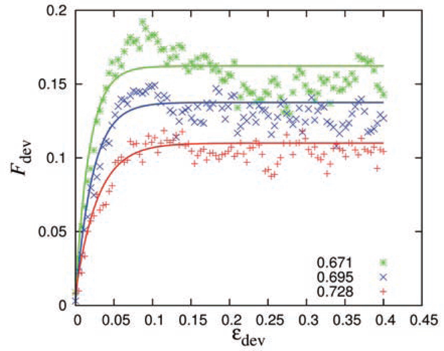
The stress-strain behavior in the case of uniaxial compression is shown in Fig. 12 star ting from initial volume fractions v =0.671, 0.695, 0.728, to a common maximum value v_max =0.820. Unlike the volume-conserving deviatoric simulations discussed previously, the evolution of the deviatoric stress ratio during uniaxial compression leads to large fluctuations that do not allow the clear observation of a possible softening/hardening regime. This difference is because the uniaxial deformation mode has a continuously increasing density and pressure in contrast, for example, to mode D3 where σ_zz is increasing and σ_yy ≈ σ_xx are decreasing such that the pressure remains (almost) constant. The solid lines superimposed on the data in the plot represent the predictions of the constitutive relation in Eq. (17), with the parameters obtained from the deviatoric modes D2 and D3, as explained in detail in section 7.

Fig. 12

Deviatoric stress ratio plotted against deviatoric strain from the uniaxial compression mode data for different initial volume fractions v_i during unloading, from which the uniaxial deformations were initiated, as given in the inset. The symbols ( ‘*’, ‘×’ and ‘+’ ) are the simulation data while the solid lines represent the prediction using Eq. (17).

Moreover, as the deviatoric strain increases during uniaxial deformation, the deviatoric stress ratio s_dev also increases with values that depend on the initial volume fraction. For lower volume fractions we observe a higher stress ratio, similar to what is observed in Fig. 11. Interestingly, uniaxial deformations for different initial volume fractions lead to convergence (and almost collapse) after about 7.5 percent deviatoric strain. This feature of the uniaxial simulations is also well captured by the anisotropy model in section 7.3.

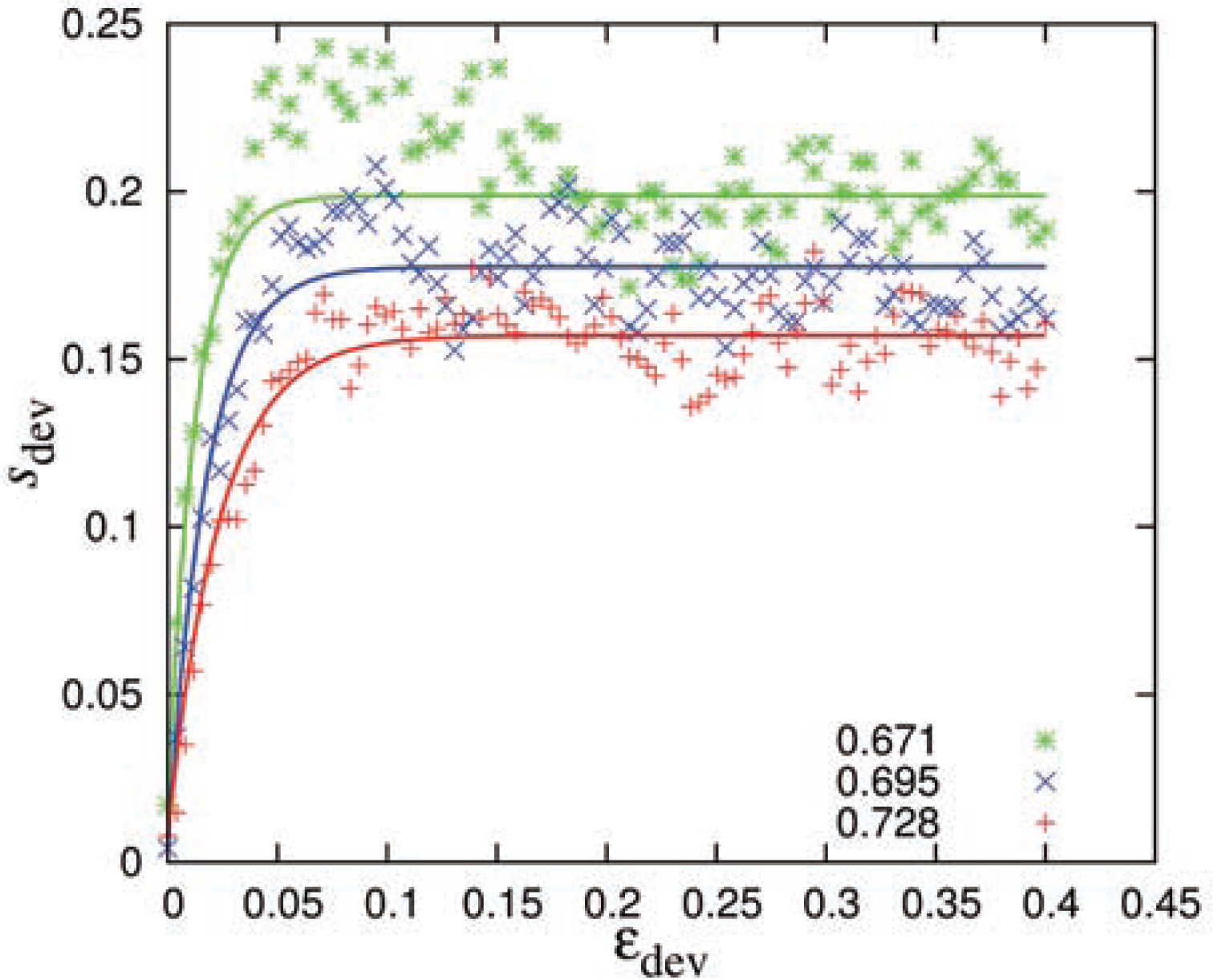
6.2.2 Deviatoric fabric

The evolution of the deviatoric fabric F_dev as a function of the deviatoric strain is shown in Fig. 13 for mode D2 simulations and three different volume fractions. It builds up from different random, small initial values and reaches different maximum saturation values $F_{\text{dev}}^{\text{max}}$. The deviatoric fabric increases faster at lower volume fractions in a very similar fashion to what was observed for the stress ratio in Fig. 11. Both the growth rate and the maximum deviatoric fabric are well defined and shown in Fig. 13 together with the fitting curves used to deduce the theoretical values β_F and $F_{\text{dev}}^{\text{max}}$ for different volume fractions (see details in section 7.2).

Fig. 13

Deviatoric fabric plotted against deviatoric strain from the D2 deformation simulations of Fig. 11 The symbols (‘*’, ‘×’ and ‘+’) are the simulation data while the solid lines through them represent a fit to the data using Eq. (18).

The evolution of the deviatoric fabric for the D3 mode is not shown since it resembles the behavior of the D2 mode, implying that the fabric evolution is pretty much insensitive to the deviatoric deformation protocol employed, as was observed before also for the stress ratio. A more detailed study of the (small) differences among deformation modes with different shape factors, as predicted by Thornton and Zhang, 2010, will be reported elsewhere.

Fig. 14 shows the evolution of the deviatoric fabric during uniaxial compression as presented in section 6.2.1. The deviatoric fabric builds up as the deviatoric strain (and the volume fraction) increases. It begins to saturate at ε_dev ≈ 0.06 and a slight decreasing (softening) trend is seen towards the end of the loading path. The convergence of the deviatoric stress after large strain, for different volume fractions, as seen in Fig. 12, does not appear so clearly for the deviatoric fabric. The theoretical prediction of the constitutive relations from section 7 is in good qualitative agreement with the numerical data, but over-predicts the deviatoric fabric for larger strains. Their analytical form and the parameters involved will be discussed next.

Fig. 14

Deviatoric fabric plotted against deviatoric strain from the uniaxial deformation simulations in Fig. 12 The symbols (‘*’, ‘×’ and ‘+’) are the simulation data while the solid lines through them represent the prediction of the data using Eq. (18).

7. Theory: Macroscopic Evolution Equations

Constitutive models are manifold and most standard models with wide application fields such as elasticity, elasto-plasticity, or fluid-/gas-models of various kinds were applied also to granular flows – sometimes with success, but typically only in a very limited range of parameters and flow conditions; for overviews see, e.g. GdR-MiDi, 2004; Luding and Alonso-Marroquín, 2011. The framework of kinetic theory is an established tool with quantitative predictive value for rapid granular flows only – but it is hardly applicable in dense, quasi-static and static situations (Luding, 2009). Further models, such as hyper- or hypo-elasticity, are complemented by hypoplasticity (Kolymbas, 1991) and the so-called granular solid hydrodynamics (Jiang and Liu, 2009), where the latter provides incremental evolution equations for the evolution of stress with strain, and involve limit states (Mašín, 2012) instead of a plastic yield surface as in plasticity theory. A strict split between elastic and plastic behavior seems invalid in granular materials, see, e.g. Alonso-Marroquín et al, 2005. More advanced models involve so-called non-associated / non-coaxial flow rules, where some assumptions on relations between different tensors are proposed, see Thornton and Zhang, 2006, 2010. While most of these theories can be or have been extended to accommodate anisotropy of the microstructure, only very few models account for an independent evolution of strain, stress and microstructure (see, for example, Thornton and Zhang, 2010; Sun and Sundaresan, 2011; Luding and Perdahcioğlu, 2011; Goddard, 2010) as found to be important in this study and many others.

In the following, we use the anisotropy constitutive model as proposed in Kumar et al., 2012a; Luding and Perdahcioğlu, 2011; Magnanimo and Luding, 2011, generalized for a 𝒟 –dimensional system:   

$$\begin{array}{l}\delta P=𝒟B\delta {ϵ}_{\text{v}}+AS\delta {ϵ}_{\text{dev}},\\ \delta {\sigma }_{\text{dev}}=A\delta {ϵ}_{\text{v}}+𝒟G^{\text{oct}}S\delta {ϵ}_{\text{dev}},\\ \delta A={\beta }_A\text{sign}\left(\delta {ϵ}_{\text{dev}}\right)\left(A^{\text{max}}-A\right)\delta {ϵ}_{\text{dev}}.\end{array}$$(16)

In its simplest form, the model involves only three moduli: the classic bulk modulus B (Göncü et al., 2010), the octahedral shear modulus G^oct, and the new variable “anisotropy modulus” A, evolving independently of stress with deviatoric strain. Due to A, the model provides a cross-coupling between the two types of stress and strain in the model, namely the hydrostatic and the shear (deviatoric) stresses react to both isotropic and deviatoric strains. $S=\left(1-s_{\text{dev}}/{\text{s}}_{\text{dev}}^{\text{max}}\right)$ is an abbreviation for the stress isotropy with $s_{\text{dev}}={\sigma }_{\text{dev}}/P$. The parameter $s_{\text{dev}}^{\text{max}}$ resembles the macroscopic friction and β_s is the growth rate of s_dev with deviatoric strain ${ϵ}_{\text{dev}}$. The parameter A^max in the evolution equation of A represents the maximum anisotropy that can be reached at saturation, and β_A determines how fast the asymptote is reached (growth rate). Both A^max and β_A are model parameters for the anisotropy modulus and can be extracted from fits to the macroscopic, average simulation results. Note that the evolution of is assumed to be kinematic, i.e. not explicitly dependent on pressure, but there is a possible volume fraction dependence of β_A and A^max, as detailed below.

In the following, we test the proposed model by extracting the model parameters as functions of volume fraction v from various volume-conserving deviatoric simulations. The calibrated model is then used to predict the uniaxial deformation behavior (see the previous section). The theory will be discussed elsewhere in more detail (Kumar et al., 2012a; Magnanimo and Luding, 2012). In short, it is based on the basic postulate that the independent evolution of stress and structure is possible. It comes together with some simplifying assumptions such as:

• (i) the new macroscopic field A is proportional to the microscopic rank-two deviatoric fabric F_dev so that they have the same non-dimensional growth rates ; β_F = β_A;
• (ii) both A and s_dev – to lowest order, i.e. neglecting additional (missing) terms in Eqs. (16) – approach their limit states exponentially fast;
• (iii) only one anisotropy modulus A is sufficient (valid in 2D, questionable in 3D, possibly two moduli A₁ and A₂ are needed);

that lead to Eqs. (17) and (18) below. We use these two equations as empirical fit functions, since they are special cases of the complete constitutive model with anisotropy, and then use the fit result to predict another solution of the (simplified) theory for another deformation mode.

7.1 Reduced theoretical model

The reduced model consists of two evolution equations for the deviatoric stress ratio s_dev related to the mobilized macroscopic friction, and the deviatoric fabric F_dev based on DEM observations in 2D, see Luding, 2004, 2005. For volume-conserving pure shear, Figs. 11 and 13 show that s_dev and F_dev grow non-linearly until they approach exponentially a constant value at steady state, with fluctuations where the material can be indefinitely sheared without further change. As discussed by Luding and Perdahcioğlu, 2011, the coupled evolution equations (16) are (with above assumptions) consistent with s_dev approximated by:   

$$s_{\text{dev}}=s_{\text{dev}}^{\text{max}}-\left(s_{\text{dev}}^{\text{max}}-s_{\text{dev}}^0\right){\text{e}}^{-{\beta }_s{ϵ}_{\text{dev}}},$$(17)

where $s_{\text{dev}}^0$ and $s_{\text{dev}}^{\text{max}}$ represent the initial and maximum values of s_dev and β_s is its growth rate. Similarly, the deviatoric fabric is approximated by:   

$$F_{\text{dev}}=F_{\text{dev}}^{\text{max}}-\left(F_{\text{dev}}^{\text{max}}-F_{\text{dev}}^0\right){\text{e}}^{-{\beta }_F{ϵ}_{\text{dev}}},$$(18)

where $F_{\text{dev}}^0$ and $F_{\text{dev}}^{\text{max}}$ represent the initial and maximum (saturation) values of the deviatoric fabric and β_F is its rate of change. To study the variation of the parameters $s_{\text{dev}}^{\text{max}}$, β_s, $F_{\text{dev}}^0$, and $F_{\text{dev}}^{\text{max}}$ with volume fraction v, during deviatoric deformation, we perform several isochoric simulations at different volume fractions v_i, and obtain the coefficients as shown in Figs. 15 and 16 from fits to Eqs. (17) and (18).

Fig. 15

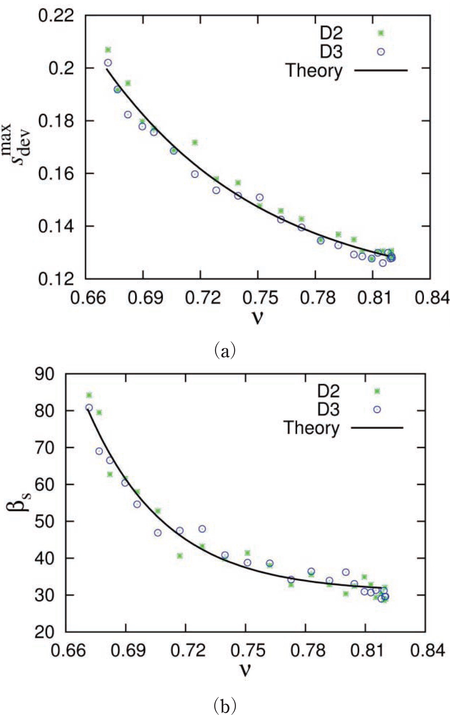
Comparison of evolution parameters from Eq. (17): the maximum normalized deviatoric stress $s_{\text{dev}}^{\text{max}}$ and the growth rate β_s plotted against volume fraction v for the D2 and D3 deviatoric modes. Each point represents a unique simulation; the green ‘*’ s represent the D2 mode while the blue ‘⊙’ s represent the D3 mode. The solid black line is the proposed analytical form in Eq. (20), with parameters given in Table 3.

Fig. 16

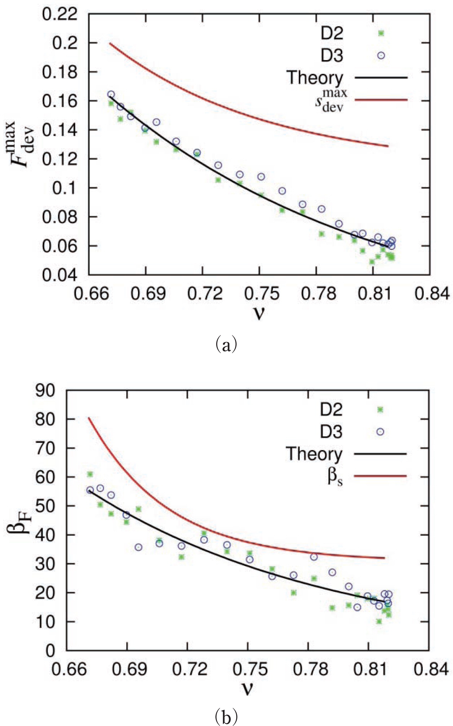
Comparison of evolution parameters from Eq. (18): the maximum anisotropy $F_{\text{max}}^{\text{dev}}$ and the growth rate β_F plotted against volume fraction v for the D2 and D3 deviatoric modes. The solid black line is the proposed theory, Eq. (20), for $F_{\text{max}}^{\text{dev}}$ and β_F, respectively, while the red lines are the corresponding parameters $s_{\text{max}}^{\text{dev}}$ and β_s in Fig. 15.

As a final step, but not shown in this paper, in order to relate the macroscopic anisotropy (modulus) A to the evolution of the deviatoric fabric F_dev, one can measure the elastic modulus A directly. For this, the sample is subjected to incremental deformations (either isotropic or purely deviatoric) at various different stages along the (large strain) deviatoric paths for D2 and D3 deformations. Details of the procedure and the results will be reported elsewhere (Kumar et al., 2012a). Here, we only note that a linear relation is found such that:   

$$A\approx a_0^{*}{F}_{\text{dev}}\frac{P{v}_c^2}{\left(\nu -{\nu }_c\right)}\approx \frac{a_{0}k}{2⟨r⟩}{F}_{\text{v}}{F}_{\text{dev}}$$(19)

where a₀ = 0.137 is a combination of numerical constants including g₃, p₀.

7.2 Fitting of deviatoric deformations: calibration of the anisotropy model

From the analysis of various deviatoric D2 and D3 simulations with different volume fractions, using Eq. (17) we obtain the variation of $s_{\text{dev}}^{\text{max}}$ and β_s with v, see Fig. 15. The factor $s_{\text{dev}}^{\text{max}}$ decreases with increasing volume fraction v and a similar trend is observed for β_s with some larger scatter. Both $s_{\text{dev}}^{\text{max}}$ and β_s seem to saturate towards a finite limit for large volume fractions, and these values can be extrapolated by the fitting procedure described later in this section. The fit procedure applied to the deformation modes D2 and D3 leads to very similar results for $s_{\text{dev}}^{\text{max}}$ and β_s. This is not surprising: the same net deviatoric strain applied in the two modes leads to (almost) the same net deviatoric stress ratio response, even though the shapes of deformations are different.

Fig. 16(a) shows the variation of $F_{\text{dev}}^{\text{max}}$ with volume fraction for the same simulations as in Fig. 15, where the two deviatoric deformation modes D2 and D3 almost collapse on each other. $F_{\text{dev}}^{\text{max}}$ decreases strongly with volume fraction v for the two modes. For higher volume fractions, the motion of spheres is more constrained by more contacts and hence the contact anisotropy developed in the system is smaller. Fig. 16(b) shows a similar decreasing behavior of β_F with volume fraction v, where stronger scatter is seen. The analytical fits of the normalized stress parameters ( $s_{\text{dev}}^{\text{max}}$ and β_s) are shown for comparison.

A different behavior of the normalized stress and the deviatoric fabric with respect to both parameters (maximum saturation value and the evolution rate) proves that stress and fabric evolve independently of deviatoric strain (La Ragione and Magnanimo, 2012), as is the basic postulate for the anisotropic constitutive model.

For the fit, we propose a generalized analytical relation for both the stress parameters $s_{\text{dev}}^{\text{max}}$, β_s and the fabric parameters $F_{\text{dev}}^{\text{max}}$, β_F. The dependence of the parameters on the volume fraction v is well described by the general relation:   

$$Q=Q_{\text{max}}+Q_{\text{v}}{\text{e}}^{\left(-\alpha \left(\frac{\nu }{{\nu }_{\text{c}}}-1\right)\right)},$$(20)

where Q_max, Q_v and α are the fitting parameters with values presented in Table 3, and v_c ≈ 0.6653 is chosen as the jamming volume fraction, see Table 2. For all four parameters, the Q_max values are the limit for large volume fractions, while Q_c = Q_max + Q_v represents the limit at v → v_c and α is the rate of variation (decay) with the volume fraction increasing above v_c. We assume, as is consistent with the data, that the structural anisotropy parameters $F_{\text{dev}}^{\text{max}}$ and β_F tend towards zero as the volume fraction increases, therefore we keep Q_max = 0 in the fitting functions. Eq. (20) represents the solid black lines shown in Figs. 15 and 16, with coefficients given in Table 3.

Table 3 Fitting coefficients for the parameters in Eqs. (17) and (18) with v_c = 0.6653

Evolution Parameters	Qmax	Qv	α
$s_{\text{dev}}^{\text{max}}$	0.1137	0.09166	7.916
βs	30.76	57.00	16.86
$F_{\text{dev}}^{\text{max}}$	0	0.1694	4.562
βF	0	57.89	5.366

7.3 Prediction of uniaxial deformation

We use the parameters determined from the deviatoric simulations presented in Table 3 to predict the behavior of uniaxial simulations in subsection 6.2, where the volume fraction is changing with deviatoric strain and hence dependence on v is needed to properly describe the deformation path.

Fig. 12 above shows the normalized deviatoric stress s_dev against the deviatoric strain ϵ_dev for uniaxial deformations starting from three different volume fractions (v = 0.671, 0.695 and 0.728), compared with the predictions of Eq. (17) with coefficients $s_{\text{dev}}^{\text{max}}$ (v) and β_s (v) taken from Eq. (20) and coefficients from Table 3. The proposed model, although in its simplified version, is able to properly capture the behavior of the material qualitatively, approaching exponentially a maximum value and then decreasing due to the volume fraction dependence of the parameters. Note that the softening present in some of the deviatoric DEM data is on purpose not plugged into the model as a constraint, which renders the softening present in the uniaxial theoretical curves in Fig. 12 as a valuable prediction of the model. Furthermore, the convergence of s_dev for uniaxial loading simulations with different initial volume fraction at large strains, as discussed in section 6.2.1, is also well captured by the theoretical model with calibrated parameters from the deviatoric simulations (where this does not happen).

Fig. 14 shows the evolution of the deviatoric fabric F_dev with deviatoric strain ϵ_dev for uniaxial deformations – as above – together with the predictions of Eqs. (18) and (20). The model is still able to qualitatively describe the behavior of the deviatoric fabric, but with up to 30 percent over-prediction. For better quantitative agreement, the complete coupled model needs to be used and possibly improved as will be presented elsewhere (Kumar et al., 2012a).

8. Conclusions and Outlook

The discrete element method has been used to investigate the bulk response of periodic, polydisperse, frictionless sphere packings in 3D, subjected to various deformation modes, in terms of both their micro-and macroscopic responses. The main goal was to present a procedure to calibrate a constitutive model with the DEM data and then to use the same to predict another independent simulation (mode). The (overly) simple linear material (model) allows us to focus on the collective/bulk response of the material to different types of strain, excluding complex effects due to normal or tangential non-linearities. Therefore, the present study has to be seen as a reference “lower limit”, and the procedure rather than the material is the main subject.

We focused on the strain-controlled loading and unloading of isotropic, uniaxial and two deviatoric (pure shear) type deformation modes (D2 and D3). Experimentally most difficult to realize is the isotropic deformation, while both uniaxial and deviatoric modes can be realized in various element tests where, however, often mixed strain- and stress-control procedures are applied. Both micro-mechanical and coarse-grained macroscopic properties of the assemblies are discussed and related to each other. The study covers a very wide range of isotropic, uni-axial and deviatoric deformation amplitudes and thus practically all volume fractions with mechanically stable packings – except for those very close to the jamming transition and higher than about 10 percent contact deformation, above which DEM pair contact models become questionable.

8.1 Microscopic quantities

The microscopic coordination number C, defined as the ratio of the total number of contacts to the total number of particles, has been analyzed as a function of volume fraction and deviatoric strain. By disregarding particles with less than four contacts (called rattlers), the corrected coordination number C^* is well described by Eq. (11) for all deformation modes (since the particles are frictionless). For the uniform size distribution used here, the fraction of rattlers shows an exponentially decaying trend towards higher volume fractions, very similar for all modes, see Eq. (12) and Table 2. These analytical relations provide a prediction for the coordination number C = (1 − ϕ_r)C^* that notably shows up in the macroscopic relations for both pressure and isotropic fabric, in combination with volume fraction v, instead of C^*. Note that C^* is better accessible to theory, while vC is related to the wave-propagation speed, which is experimentally accessible, while both are linked by the fraction of rattlers, which was already identified as a control parameter of utmost importance (Bi et al., 2011).

A small but systematic difference in C^* and ϕ_r parameters appears for the different deformation modes. Most important, the jamming volume fraction v_c is not a single, particular volume fraction, but we observe a range of jamming volume fractions dependent on the deformation modes, i.e. the “history” of the sample. Over-compression leads to an increase of v_c, i.e. to a better, more efficient packing. Subsequent deviatoric (pure shear) deformations slightly reduce the jamming volume fraction of such a previously over-compressed packing, causing it to become less efficiently packed. Thus more/less efficient packing is reflected by a large/small jamming volume fraction and, inversely, small/large coordination numbers. The observed differences are more pronounced as the volume fraction becomes lower. A slight increase in the fraction of rattlers due to deviatoric deformations is also reported, as consistent with the decrease in coordination number.

8.2 Macroscopic quantities

When focusing on macroscopic quantities, an important result from this study is that at small strains, the uniaxial, deviatoric and isotropic modes can be described by the same analytical pressure evolution, Eq. (15), with parameters given in Table 2, evidenced by the collapse of the data from these deformation modes when the scaled pressure is plotted as a (linear) function of the volumetric strain.

This linearity is due to the scaling with the nonlinear terms p^* ∝ p/(vC) in particular. Thanks to the linear contact model used, it allows the conclusion that the non-linear (quadratic) corrections are due to the structural rearrangements and non-affine deformations. The scaled deviatoric and uniaxial results deviate from the isotropic pressure data. This appears at larger strains due to the build-up of anisotropy in the system, caused by deviatoric strain, obviously not present in the isotropic deformation mode. The good match of the data suggests an advantage of the “cheaper” uniaxial (and deviatoric) deformation modes over the experimentally difficult to realize isotropic deformation mode (three walls have to be moved simultaneously in the isotropic case, while a less complicated set-up is required for the other modes).

The deviatoric stress ratio (the deviatoric stress scaled with the isotropic pressure) as a function of the deviatoric strain develops almost independently of the volume fraction when the deviatoric magnitude is defined in a similar fashion to the second deviatoric invariant (Thornton and Zhang, 2006) for all quantities studied. The deviatoric stress builds up with increasing deviatoric strain until a steady state is reached (where we do not focus on peak and softening behavior, which becomes more pronounced when the jamming volume fraction is approached). Starting from isotropic initial configurations, we also show that the slope G^oct/P of the normalized deviatoric stress as a function of deviatoric strain decreases with increasing volume fraction, unlike the shear modulus G^oct, which increases with volume fraction. This indicates that the pressure (and bulk modulus B) has a “stronger” dependence on the volume fraction than the shear modulus.

From the macroscopic data, one observes that deviatoric and isotropic stresses and strains are cross-coupled by the structural anisotropy. The latter is quantified by the deviatoric fabric, which is proportional to the bulk anisotropy modulus/moduli A, as relevant for the constitutive model. Cross-coupling means that in the presence of structural anisotropy, isotropic strain can cause deviatoric stress responses and deviatoric strain can cause isotropic stress responses (dilatancy or compactancy). The structural anisotropy response to deviatoric strain is very similar to that of the deviatoric stress ratio. The response rates of both stress and structure anisotropies with deviatoric strain are functions of volume fraction and, most important, are different from each other.

8.3 Constitutive model calibration

As a first step, the parameters of a simple constitutive model that involves anisotropy as proposed for 2D by Luding and Perdahcioğlu, 2011, Magnanimo and Luding, 2011 have been calibrated from DEM data. From the isotropic deformation mode, one can extract the bulk modulus B, as was done by Göncü et al., 2010. From the volume-conserving D2 and D3 modes, by fitting the idealized evolution equations for shear stress in Eq. (17), the macroscopic friction $s_{\text{dev}}^{\text{max}}$ and the deviatoric stress rate β_s can be inferred as functions of the volume fraction, entering the shear modulus G^oct. Similarly, the fit of Eq. (18) provides a relation for the maximum fabric anisotropy at steady state $F_{\text{dev}}^{\text{max}}$ and the fabric rate β_F as functions of volume fraction. A relation between the deviatoric fabric and the anisotropy modulus/moduli A in the model is finally needed to close the system and allow integration of the coupled evolution equations for stress and structure.

As a second step and major result, the constitutive model calibrated on deviatoric data has been used to predict qualitatively (and to some extent also quantitatively) both stress and fabric evolution under uni-axial deformation. This is very promising, since the basic qualitative features are caught by the model, even though it was used in a very idealized and short form, with the single anisotropy modulus A ∝ F_dev the only main new ingredient. Several additional terms of assumed minor impact are ignored and have to be added to complete the model, see Kumar et al., 2012a; Magnanimo and Luding, 2011; Sun and Sundaresan, 2011; Thornton and Zhang, 2010, and references therein, as postponed to future studies. (For example, an objective tensorial description of stress, strain and fabric involves also the third tensor invariants. Alternatively/equivalently, these deviatoric tensors can be completely classified by the shape factors in their respective eigen-systems, which allow us to distinguish all possible deformation and response modes in 3D.)

8.4 Outlook

In this paper, we have reviewed and presented new results for frictionless particles undergoing isotropic, uniaxial, and (pure) shear deformation. Since the particles are too idealized here, the results cannot be applied to practical systems where shape, friction, and other non-linearities are relevant. However, they form the basic reference study with details given on the calibration procedure that yields a constitutive model with satisfactory predictive quality. Therefore, the next steps in our research will involve more realistic contact models with friction, cohesion, and other physically meaningful material parameters. Only then can the validity of the analytical expressions be tested for realistic systems, to predict well the phenomenology for pressure as well as the scaling arguments for the deviatoric stress and fabric.

Laboratory element test experiments should also be performed with the biaxial box to validate the simulation results with realistic material properties. Macroscopic quantities that can be readily obtained experimentally – for example, the pressure-volume fraction relation and the shear stress evolution with deviatoric (pure shear) strain – can then be compared with simulation data. Moreover, the work underlines the predictive power of constitutive models with anisotropy (as in Luding and Perdahcioğlu, 2011; Magnanimo and Luding, 2011; Sun and Sundaresan, 2011) that can be further tested, validated and extended with more advanced physical and numerical experiments.

Given the detailed insights from DEM, the (missing) terms and the parameters for the constitutive models can now be further analyzed to perform the rigorous micro-macro transition.

Open questions concern, among others:

• (i) the validity of the 2D model in 3D, related to missing terms and parameters,
• (ii) the validity of global versus local coarse-graining, i.e. the scale of the micro-macro transition (Kuhn and Bagi, 2009),
• (iii) the microscopic (restructuring) and macroscopic (non-affine motions) origin of the peak and softening phenomenology at low volume fractions, possibly related to the (in)homogeneity of the packings,
• (iv) the validity of the model predictions for strain-reversal and cyclic deformations, and
• (v) the possible dependence of the moduli in the constitutive relations on other quantities (e.g. pressure) than the volume fraction, as focused on in this study.

For future application, the present calibration procedure should be checked also for other materials and applied to different element tests, among which there are (cylindrical) triaxial tests, ring-shear tests and also avalanche flow experiments like in chutes or rotating drums, all of which are more widely available than the “academic” biaxial box. In the end, the material properties and parameters should not depend on the element test chosen and the predictive value of the model(s) should be proven for more than only one validation test, be it another element test or a real-size or lab-scale process such as, e.g. granular flow in a silo or during a landslide.

Acknowledgements

Helpful discussions with F. Göncü, J. Ooi, M. B. Wojtkowski and M. Ramaioli are gratefully acknowledged. This work is financially supported by the European-Union-funded Marie Curie Initial Training Network, FP7 (ITN-238577), see http://www.pardem.eu/ for more information.

Author’s short biography

Olukayode I. Imole

Olukayode I. Imole completed his BEng degree in mechanical engineering at the University of Ado-Ekiti, Nigeria. He received the DAAD scholarship to study for a MSc degree in quality, safety and environment at the Otto-von-Guericke University, Magdeburg, Germany, where he worked with the mechanical process engineering group chaired by Prof. Jürgen Tomas. His master’s thesis was titled “Investigation of the kinetics of disintegration processes during titania nanoparticle synthesis”. He is presently on a Marie Curie fellowship for his PhD in the multi-scale mechanics group, Faculty of Engineering Technology (CTW), chaired by Prof. Stefan Luding at the University of Twente, Netherlands. His research interests include experimental work on element tests with focus on cohesive powders, discrete element simulations of frictionless, frictional and cohesive granular assemblies and other industry-relevant research. He collaborates with other researchers in various institutions and industries including TU Braunschweig, Germany, UT Compiegne, France, and Nestle Research, Switzerland.

Nishant Kumar

Nishant Kumar is a PhD student in the multi-scale mechanics (MSM) group at the faculty of Engineering Technology, CTW, University of Twente, Netherlands. He finished his B.Tech. degree in Chemical engineering at the Indian Institute of Technology (IIT), Kanpur, in 2008. He received his MS with honors in Mechanical engineering from the University of California, San Diego (UCSD), in 2008. Later, he joined the MSM group in 2010. His research interests include the constitutive modeling of materials with an internal micro-structure such as soils and cohesive powders and his focus is on anisotropy models. He is also working on shear jamming in granular materials.

Vanessa Magnanimo

Vanessa Magnanimo is assistant professor in the multi-scale mechanics (MSM) group at the faculty of Engineering Technology, CTW, University of Twente, Netherlands. She received a MSc degree in construction engineering from the Politecnico of Bari, Italy, with subsequent graduate studies on the elasticity of discrete materials. In 2007 she received her PhD in continuum mechanics from the same university. She was a visiting scientist at the Levich Institute - CCNY (2005) and at T&AM - Cornell University (2008). Her research interests concern theoretical analysis and modern simulation techniques applied to sound propagation and the constitutive modeling of materials with an internal micro-structure such as soils, asphalt, powders and bio-materials.

Stefan Luding

Stefan Luding studied physics at the University of Bayreuth, Germany, focusing on reactions on complex and fractal geometries. He continued his research in Freiburg for his PhD on simulations of dry granular materials in the group of Prof. A. Blumen. He spent his post-doctorate time in Paris IV, Jussieu, with E. Clement and J. Duran before he joined the computational physics group with Prof. Herrmann for his habilitation. In 2001, he moved to DelftChemTech at the TU Delft in Netherlands as associate professor for particle technology. Since 2007 he has held the chair on multi-scale mechanics (MSM) at the Faculty of Engineering Technology, CTW, at the University of Twente, Netherlands, with ongoing research on fluids, solids, particle interactions, granular materials, powders, asphalt, composites, bio- and micro-fluid systems and self-healing materials. Stefan Luding has been managing editor in chief of the journal Granular Matter since 1998. He has written more than 200 publications and is a member of several international working parties, including presidentship of AEMMG that organizes the Powders and Grains Conference in 2009 and 2013.

References

•  Alonso-Marroquín,  F.;  Luding,  S.;  Herrmann,  H. J. and  Vardoulakis,  I. (2005): “Role of anisotropy in the elastoplastic response of a polygonal packing.” Phyical Review E., 71:051304:1–18.
•  Barreto,  D. and  O’Sullivan,  C. (2012): “The influence of inter-particle friction and the intermediate stress ratio on soil response under generalised stress conditions.” Granular Matter, 14(4):505–521.
•  Bi,  D.;  Zhang,  J.;  Chakraborty,  B. and  Behringer,  R. P. (2011): “Jamming by shear.” Nature, 480(7377):355–358.
•  Cundall,  P. A. and  Strack,  O. D. L. (1979): “A discrete numerical model for granular assemblies.” Géotechnique, 29(1):47–65.
•  Durán,  O.;  Kruyt,  N. P. and  Luding,  S. (2010): “Micro-mechanical analysis of deformation characteristics of three-dimensional granular materials.” International Journal of Solids and Structures, 47(17):2234–2245.
•  Ezaoui,  A. and  Di Benedetto,  H. (2009): “Experimental measurements of the global anisotropic elastic behaviour of dry Hostun sand during triaxial tests, and effect of sample preparation.” Géotechnique, 59(7):621–635.
•  Fredlund,  D. G. (1979): “Second Canadian Geotechnical Colloquium: Appropriate concepts and technology for unsaturated soils.” Canadian Geotechnical Journal, 16(1):121–139.
• GdR-MiDi. (2004): “On dense granular flows.” The European Physical Journal E: Soft Matter and Biological Physics, 14(4):341–365.
•  Goddard,  J. D. (1998): “Continuum Modeling of Granular Assemblies.” In  Herrmann,  H. J.;  Hovi,  J. P. and  Luding,  S. editors, Physics of dry granular media - NATO ASI Series E 350, pages 1–24, Dordrecht, Kluwer Academic Publishers.
•  Goddard,  J. D. (2010): “Parametric hypoplasticity as continuum model for granular media: from Stokesium to Mohr-Coulombium and beyond.” Granular Matter, 12:145–150.
•  Göncü,  F.;  Duran,  O. and  Luding,  S. (2010): “Constitutive relations for the isotropic deformation of frictionless packings of polydisperse spheres.” C. R. Mécanique, 338(10–11):570–586.
•  Hayhurst,  D. R. (1972): “Creep rupture under multi-axial states of stress.” Journal of the Mechanics and Physics of Solids, 20(6):381–382.
•  Hertz,  H. (1881): “Über die Berührung fester elastischer Körper.” Journal für die Reinen und Angewandte Mathematik, 92:156–171.
•  Imole,  O. I.;  Kumar,  N. and  Luding,  S. (2011): “Deformation modes of packings of frictionless polydisperse spheres.” Particulate Systems Analysis Conference Proceedings, pages 1–6.
•  Jiang,  Y. and  Liu,  M. (2009): “Granular solid hydrodynamics.” Granular Matter, 11:139–156.
•  Kolymbas,  D. (1991): “An outline of hypoplasticity.” Archive of Applied Mechanics, 61:143–151.
•  Kruyt,  N. P.;  Agnolin,  I.;  Luding,  S. and  Rothenburg,  L. (2010): “Micromechanical study of elastic moduli of loose granular materials.” Journal of the Mechanics and Physics of Solids, 58(9):1286–1301.
•  Kuhn,  M. R. and  Bagi,  K. (2009): “Specimen Size Effect in Discrete Element Simulations of Granular Assemblies.” Journal of Engineering Mechanics, 135(6):485–492.
•  Kumar,  N.;  Imole,  O. I.;  Magnanimo,  V. and  Luding,  S. (2012a): “Predictive methods for deformation modes using constitutive modeling for frictionless spheres: Micro-macro transition to an Anisotropy model.” In preparation.
•  Kumar,  N.;  Imole,  O. I.;  Magnanimo,  V. and  Luding,  S. (2012b): “Deformation Modes for Assemblies of Frictionless Polydisperse Spheres.” Advanced Materials Research, 508:160–165.
•  Kwade,  A.;  Schulze,  D. and  Schwedes,  J. (1994): “Determination of the stress ratio in uniaxial compression tests - Part 2.” Powder Handling & Processing, 6(2):199–203.
•  La Ragione,  L. and  Magnanimo,  V. (2012): “Contact anisotropy and coordination number for a granular assembly: A comparison of distinct element method simulations and theory.” Phyical Review E., 85:031304:1–8.
•  Luding,  S. (2004): “Micro-Macro Models for Anisotropic Granular Media.” In  Vermeer,  P. A.;  Ehlers,  W.;  Herrmann,  H. J. and  Ramm,  E. editors, Modelling of Cohesive-Frictional Materials, pages 195–206, Leiden, Netherlands, Balkema.
•  Luding,  S. (2005): “Anisotropy in cohesive, frictional granular media.” Journal of Physics: Condensed Matter, 17(24):S2623–S2640.
•  Luding,  S. (2008a): “Constitutive relations for the shear band evolution in granular matter under large strain.” Particuology, 6(6):501–505.
•  Luding,  S. (2008b): “The effect of friction on wide shear bands.” Particulate Science and Technology, 26(1):33–42.
•  Luding,  S. (2008c): “Cohesive, frictional powders: contact models for tension.” Granular Matter, 10(4):235–246.
•  Luding,  S. (2009): “Towards dense, realistic granular media in 2D.” Nonlinearity, 22(12):R101–R146.
•  Luding,  S. and  Alonso-Marroquín,  F. (2011): “The critical-state yield stress (termination locus) of adhesive powders from a single numerical experiment.” Granular Matter, 13(2):109–119.
•  Luding,  S.;  Perdahcioğlu,  E. S. (2011): “A Local Constitutive Model with Anisotropy for Various Homogeneous 2D Biaxial Deformation Modes.” Chemie Ingenieur Technik, 83(5):672–688.
•  Magnanimo,  V.;  La Ragione,  L.;  Jenkins,  J. T.;  Wang,  P. and  Makse,  H. A. (2008): Characterizing the shear and bulk moduli of an idealized granular material, Europhysics Letters, 81(3):34006:1–6.
•  Magnanimo,  V. and  Luding,  S. (2011): “A local constitutive model with anisotropy for ratcheting under 2D axial-symmetric isobaric deformation.” Granular Matter, 13(3):225–232.
•  Magnanimo,  V. and  Luding,  S. (2012): “A 2D non-linear constitutive model with anisotropy for granular materials.”, Philosophical Magazine, (Under review).
•  Majmudar,  T. S.;  Sperl,  M.;  Luding,  S. and  Behringer,  R. P. (2007): “Jamming Transition in Granular Systems.” Phyical Review Letters, 98(5):058001:1–4.
•  Makse,  H. A.;  Johnson,  D. L. and  Schwartz,  L. M. (2000): “Packing of compressible granular materials.” Phyical Review Letters, 84(18):4160–4163.
•  Mašín,  D. (2012): “Asymptotic behaviour of granular materials.” Granular Matter, 14:759–774.
•  Maxwell,  J. C. (1864): “On the calculation of the equilibrium and stiffness of frames.” Philosophical Magazine, 27(182):598–604.
•  Mindlin,  R. D. and  Deresiewicz,  H. (1953): “Elastic spheres in contact under varying oblique forces.” Journal of Applied Mechanics, 75:327–344.
•  Morgeneyer,  M. and  Schwedes,  J. (2003): “Investigation of powder properties using alternating strain paths.” Task Quarterly, 7(4):571–578.
•  Oda,  M. (1972): “Initial fabrics and their relations to mechanical properties of granular material.” Soil and foundations, 12(1):17–36.
•  O’Hern,  C. S.;  Langer,  S. A.;  Liu,  A. J. and  Nagel,  S. R. (2002): “Random packings of frictionless particles.” Phyical Review Letters, 88(7):075507:1–4.
•  Philippe,  P.;  Bonnet,  F. and  Nicot,  F. (2011): “Settlement of a granular material: boundary versus volume loading.” Granular Matter, 13(5):585–598.
•  Radjai,  F.;  Roux,  S. and  Moreau,  J. J. (1999): “Contact forces in a granular packing.” Chaos, 9(3):544–550.
•  Saadatfar,  M.;  Sheppard,  A. P.;  Senden,  T. J. and  Kabla,  A. J. (2012): “Mapping forces in a 3D elastic assembly of grains.” Journal of the Mechanics and Physics of Solids, 60(1):55–66.
•  Samimi,  A.;  Hassanpour,  A. and  Ghadiri,  M. (2005): “Single and bulk compressions of soft granules: Experimental study and DEM evaluation.” Chemical Engineering Science, 60(14):3993–4004.
•  Schwedes,  J. (2003): “Review on testers for measuring flow properties of bulk solids.” Granular Matter, 5(1):1–43.
•  Shaebani,  M. R.;  Madadi,  M.;  Luding,  S. and  Wolf,  D. E. (2012): “Influence of polydispersity on micromechanics of granular materials.” Phyical Review E., 85(1):011301:1–12.
•  Spencer,  A. J. M. (1980): Continuum mechanics. Dover Publishers, USA.
•  Sun,  J. and  Sundaresan,  S. (2011): “A constitutive model with microstructure evolution for ow of rate independent granular materials.” Journal of Fluid Mechanics, 682:590–616.
•  Thornton,  C. (2010): “Quasi-static simulations of compact polydisperse particle systems.” Particuology, 8(2):119–126.
•  Thornton,  C. and  Anthony,  S. J. (1998): “Quasistatic deformation of particulate media.” Philosophical Transactions of the Royal Society of London, Series A: Mathematical, Physical and Engineering Sciences, 356(1747):2763–2782.
•  Thornton,  C. and  Zhang,  L. (2006): “A numerical examination of shear banding and simple shear non-coaxial flow rules.” Philosophical Magazine, 86(21–22):3425–3452.
•  Thornton,  C. and  Zhang,  L. (2010): “On the evolution of stress and microstructure during general 3D deviatoric straining of granular media.” Géotechnique, 60(5):333–341.
•  van Hecke,  M. (2009): “Jamming of soft particles: geometry, mechanics, scaling and isostaticity.”, Journal of Physics: Condensed Matter, 22(3):033101:1–24.
•  Walsh,  S. D. C. and  Tordesillas,  A. (2004): “A thermomechanical approach to the development of micropolar constitutive models of granular media.” Acta Mechanica, 167(3):145–169.
•  Yimsiri,  S. and  Soga,  K. (2010): “DEM analysis of soil fabric effects on behaviour of sand.” Géotechnique, 60(6):483–495.
•  Weinhart,  T.;  Thornton,  A. R.;  Luding,  S. and  Bokhove,  O. (2012): “From discrete particles to continuum fields near a boundary.” Granular Matter, 14(2):289–294.
•  Zetzener,  H. and  Schwedes,  J. (1998): “Deformation behaviour and relaxation of bulk solids at different deformation rates.” In proceedings of the 6th International Conference on Handling and Transportation, Australia. pages 51–55.
•  Zhao,  X. and  Evans,  T. M. (2011): “Numerical analysis of critical state behaviors of granular soils under different loading conditions.” Granular Matter, 13(6):751–674.