Dense Discrete Phase Model Coupled with Kinetic Theory of Granular Flow to Improve Predictions of Bubbling Fluidized Bed Hydrodynamics

Abstract

Formation, expansion, and breakage of bubbles in single bubble and freely bubbling fluidized beds were studied using an improved hybrid Lagrangian-Eulerian computational fluid dynamics (CFD) approach. Dense Discrete Phase Model (DDPM) is a novel approach to simulate industrial scale fluidized bed reactors with polydispersed particles. The model uses a hybrid Lagrangian-Eulerian approach to track the particle parcels (lumping several particles in one computational cell) in a Lagrangian framework according to Newton’s laws of motion. The interactions between particles are estimated by the gradient of solids stress solved in Eulerian grid. In this work, a single bubble fluidized bed and a freely bubbling fluidized bed were simulated using DDPM coupled with kinetic theory of granular flows (KTGF). The solid stress was improved to include both tangential and normal forces compared to current hybrid methods with the consideration of only normal stress or solid pressure. The results showed that solid pressure (normal forces) as the only contributor in solid stress would lead to overprediction of bubble size and overlooking of bubble breakage in a single bubble bed. Also, the results showed the improved model had a good prediction of bubble path in a freely bubbling bed compared to solid pressure-based model. It was shown that increasing the restitution coefficient increased the particle content of the bubbles and it lead to less breakage during the formation of the bubble. The probability of formation of bubbles was compared with experimental results and solid stress model showed less discrepancies compared to the solid pressure-based model.

1. Introduction

The vigorous mixing of powders and granules by means of a fluidization agent has introduced the fluidized beds as one of the best tools for powder processing specially when high heat and mass transfer rates are needed (Grace, 1990; Kunii and Levenspiel, 1991). However, design and scale up of fluidized beds are difficult due to the complex hydrodynamics for a bed charged with different particles and their interactions at different operating conditions (Cocco et al., 2017).

Mathematical modeling of fluidized beds can simplify the design procedure and scale up of the fluidized beds in a cost-effective approach (Cocco et al., 2017). Modeling of a fluidized bed was initially performed by fluidization models in which the bed is divided into two emulsion and bubble phases and semi-empirical correlations were used to predict the hydrodynamics properties such as bubble size and rising velocity, gas and solid volume fraction (Davidson and Harrison, 1966; Hashemi Sohi et al., 2012). These models are good to predict the outlet composition of the fluidized bed products, and can be integrated to the chemical plant process simulations (Singhal et al., 2017).

Recently, computational fluid dynamics (CFD) models attracted the attentions for the simulation of fluidized bed systems due to the progress in computational speed by the means of parallel computation in multiple CPUs and GPUs (Norouzi et al., 2017). There are two major CFD methods to simulate fluidized beds called Eulerian-Eulerian and Eulerian-Lagrangian. Eulerian-Eulerian methods consider both gas phase and solid phase as continuous phases and add the granular properties of the solid phase using with kinetic theory of granular flows (KTGF) (Ding and Gidaspow, 1990). These methods are good for the simulation of uniform particle systems in the reactors up to a pilot scale. Several researches have been conducted to reduce mesh dependency of these methods in a large scale using filter approaches and extending application of these methods to polydisperse systems using mass balance equations (Igci et al., 2008; Radl and Sundaresan, 2014). On the other hand, Eulerian-Lagrangian methods consider a gas phase as a continuous phase and track the particles using newton laws. There are several ways to model the collisions between particles. Discrete element method (DEM) is the most accurate one in which spring dash soft sphere approach is used to model the particle collisions (Tsuji et al., 1993). However, it is impossible to simulate a large scale fluidized bed with billions of particle collisions. Therefore, different methods have been used to reduce the computational time (Benyahia and Galvin, 2010). Simplifying the collision between the particles and reducing the number of particles by grouping them into parcels are two major solutions. In the latter one, actual particles are grouped into computational parcels that are tracked in the Lagrangian framework. The event driven hard sphere and time driven hard sphere methods are simplified collision methods suffering from complex algorithm to search for particle-particle collisions in dense and polydisperse systems (Hoomans et al., 1996).

There is another approach to simplify the collisions using solid stress from Eulerian framework. In this method, the particle volume faction and velocity are mapped to the Eulerian grid and the solid stress tensor is calculated and mapped back to the particles. This approach has been used by several authors to study large scale fluidized beds for different applications due to their low computational cost. The most widely used method is called MP-PIC in which isotropic normal stress acting on each particle replaced the collisions (Fotovat et al., 2015; Snider, 2007).

  

$${\overline{\overline{\tau }}}_{\text{p}}=\frac{P_{\text{s}}{\theta }_{\text{p}}^{\beta }}{\text{max}\left[\left({\theta }_{\text{cp}}-{\theta }_{\text{p}}\right),\varepsilon \left(1-{\theta }_{\text{p}}\right)\right]}$$(1)

Where P_s is a positive constant with pressure unit, θ_p is the particle volume fraction, θ_cp is the particle volume fraction at close packing, β is a constant number arbitrarily specified with recommended values in the range 2 to 5, ɛ parameter is a small number to avoid singularity at close packing limits (Fotovat et al., 2015). Isotropic normal stress can avoid the particles from exceeding the maximum packing limit, but it does not consider the shear stresses. There are some studies in the literature reported that this approach caused weak prediction of the bubbling flow pattern in the bubbling fluidized beds (Liang et al., 2014; Lu et al., 2017).

On the other hand, Popoff and Braun (2007) introduced a dense discrete phase model in which, solid stress was calculated using kinetic theory of granular flows in Eulerian framework. However, the collision term in their work contained only the pressure like contributions (Normal pressure) of the complete stress tensor:

  

$$F_{\text{collision}}=\frac{\nabla ·p_{\text{p}}}{\rho }$$(2)

Where p_p is the solid pressure, and ρ is the solid density.

This leads to unrealistic predictions at areas close to packing limit that occur in bubbling fluidized beds and high granular temperatures. Cloete et al. have studied the effect of shear and normal forces in a DDPM model on dilute systems with periodic boundary conditions (Cloete et al., 2012). However, the effect of shear and normal forces have not yet been studied in real physical systems specifically bubbling fluidized beds. Therefore, the tangential forces were added to the model to improve the DDPM model. Their effects on the formation of bubbles and hydrodynamics of bubbling beds were studied in this work.

2. Hybrid model equations

The mass and momentum conservation equations for the gas phase are given by:

  

$$\frac{\partial ({\varepsilon }_{\text{g}}{\rho }_{\text{g}})}{\partial t}+\nabla ·({\varepsilon }_{\text{g}}{\rho }_{\text{g}}{\overrightarrow{v}}_{\text{g}})=0$$(3)

and

  

$$\begin{array}{c}\frac{\partial \left({\varepsilon }_{\text{g}}{\rho }_{\text{g}}{\overrightarrow{v}}_{\text{g}}\right)}{\partial t}+\nabla ·\left({\rho }_{\text{g}}{\overrightarrow{v}}_{\text{g}}{\overrightarrow{v}}_{\text{g}}\right)=-{\varepsilon }_{\text{g}}\nabla p_{\text{g}}+\nabla ·{\overline{\overline{\tau }}}_{\text{g}}\\ +{\varepsilon }_{\text{g}}{\rho }_{\text{g}}\overrightarrow{g}+K_{\text{DPM}}\left({\overrightarrow{v}}_{\text{DPM}}-{\overrightarrow{v}}_{\text{g}}\right)\end{array}$$(4)

where ɛ_g is the volume fraction of gas phase, ${\rho }_{\text{g}}$ is the density of gas phase, ${\overrightarrow{v}}_{\text{g}}$ is the gas phase velocity, p_g is the pressure of gas phase, ${\overline{\overline{\tau }}}_{\text{g}}$ is the shear tensor of the gas phase, K_DPM is the drag coefficient that can be calculated using a Gidaspow drag model (Ding and Gidaspow, 1990), ${\overrightarrow{v}}_{\text{DPM}}$ is the particle averaged velocity of the discrete phase mapped to the cell center.

Particle velocity and position is calculated from Newton’s law:

  

$$\frac{\text{d}{\overrightarrow{v}}_{\text{p}}}{\text{d}t}=F_{\text{D}}\left({\overrightarrow{v}}_{\text{g}}-{\overrightarrow{v}}_{\text{p}}\right)+\frac{\overrightarrow{g}\left({\rho }_{\text{p}}-{\rho }_{\text{g}}\right)}{{\rho }_{\text{p}}}+{\overrightarrow{F}}_{\text{interaction}}$$(5)

Where ${\overrightarrow{v}}_{\text{g}}$ is the gas velocity, ${\overrightarrow{v}}_{\text{p}}$ is the particle velocity, F_D stands for drag force, and ${\overrightarrow{v}}_{\text{interaction}}$ is the collision force between two particles calculated from:

  

$${\overrightarrow{F}}_{\text{interaction}}=\frac{1}{{\rho }_{\text{p}}}\nabla ·{\overline{\overline{\tau }}}_{\text{p}}$$(6)

In the above equation, ${\overline{\overline{\tau }}}_{\text{p}}$ is a solid stress including solid pressure, normal stress, and shear stress:

  

$${\overline{\overline{\tau }}}_{\text{p}}=-p_{\text{p}}\overline{\overline{I}}+{\varepsilon }_{\text{p}}{\text{μ}}_{\text{p}}\left(\nabla {\overrightarrow{v}}_{\text{p}}+\nabla {\overrightarrow{v}}_{\text{p}}^T\right)+{\varepsilon }_{\text{p}}\left({\lambda }_{\text{p}}-\frac{2}{3}{\text{μ}}_{\text{p}}\right)\nabla ·{\overrightarrow{v}}_{\text{p}}\overline{\overline{I}}$$(7)

where p_p, μ_p, and λ_p are solid pressure, shear viscosity, and bulk viscosity, respectively.

p_p is the solid pressure defined as:

  

$$p_{\text{p}}={\varepsilon }_{\text{p}}{\rho }_{\text{p}}\mathit{\Theta }+2{\rho }_{\text{p}}\left(1+e_{\text{pp}}\right){\varepsilon }_{\text{p}}{g}_0\mathit{\Theta }$$(8)

where first term is kinetic part and second term is collision part and ɡ₀ is the radial distribution function that modifies the probability of collisions between particles in dense areas:

  

$$g_0={\left[1-{\left(\frac{{\varepsilon }_{\text{p}}}{{\varepsilon }_{\text{p},\text{max}}}\right)}^{\frac{1}{3}}\right]}^{-1}$$(9)

The bulk viscosity is defined by (Lun et al., 1984):

  

$${\lambda }_{\text{p}}=\frac{4}{3}{\varepsilon }_{\text{p}}{\rho }_{\text{p}}{d}_{\text{p}}{g}_0(1+e_{\text{pp}}){(\frac{\mathit{\Theta }}{\mathrm{\pi }})}^{1/2}$$(10)

The shear viscosity is defined by (Gidaspow, 1994):

  

$$\begin{array}{c}{\mathrm{\mu }}_{\text{p}}=\frac{10{\rho }_{\text{p}}{d}_{\text{p}}\sqrt{\mathit{\Theta }\mathrm{\pi }}}{96{\varepsilon }_{\text{p}}{g}_0(1+e_{\text{pp}})}{\left[1+\frac{4}{5}{\varepsilon }_{\text{p}}{g}_0(1+e_{\text{pp}})\right]}^2\\ +\frac{4}{5}{\varepsilon }_{\text{p}}{\rho }_{\text{p}}{d}_{\text{p}}{g}_0(1+e_{\text{pp}}){(\frac{\mathit{\Theta }}{\mathrm{\pi }})}^{1/2}\end{array}$$(11)

where first term is kinetic part and second term is collisional part and Θ is granular temperature representing the kinetic energy of the fluctuating particles derived from kinetic theory model as:

  

$$\begin{array}{l}\frac{3}{2}\left[\frac{\partial \left({\varepsilon }_{\text{p}}{\rho }_{\text{p}}\mathit{\Theta }\right)}{\partial t}+\nabla ·\left({\varepsilon }_{\text{p}}{\rho }_{\text{p}}{\overrightarrow{v}}_{\text{p}}\mathit{\Theta }\right)\right]\\ ={\overline{\overline{\tau }}}_{\text{p}}:\nabla {\overrightarrow{v}}_{\text{p}}+\nabla ·\left(k_{\mathit{\Theta }}\nabla \mathit{\Theta }\right)-{\gamma }_{\mathit{\Theta }}+{\phi }_{\text{pg}}\end{array}$$(12)

Equation (10) was solved algebraically by neglecting the convection and diffusion terms in the transport equation.

2.1 Simulation setup

The simulation setup has been created based on a single bubble injected by a jet in a fluidized bed at incipient fluidization conditions and a free bubbling fluidized bed with a uniform distributor to study the effect of solid stress on single and multiple bubbles. A fluidized bed of 0.57 m width, 0.005 m depth and 1.0 m height was initially filled with glass beads at a diameter of 500 μm and a density of 2660 kg m⁻³ up to a height of 0.5 m. The background velocity for the whole bed was chosen to be 0.3 ms⁻¹ to keep the bed close to its minimum fluidization velocity and a central jet with the velocity of 10 ms⁻¹ was used to create the single bubble inside the bed (Kuipers, 1990). The computational column consists of 22903 quad cells. The second study was on a freely bubbling fluidized bed of 0.5 m width, 0.005 m depth and 1.0 m height filled with ballotini glass particles at a diameter of 700 μm and density of 2500 kg m⁻³ up to height of 0.3 m. The superficial gas velocity for bubbling fluidization was 0.62 ms⁻¹, which equals to 1.75 times of the minimum fluidization velocity (Hernández, 2013). The computational column consists of 12600 cells. The rest of operating conditions can be found in the Table 1.

Table 1 Simulation parameters.

Quantity	Unit	Single bubble jet	Freely bubbling bed
Column dimensions	m	0.57 × 1 × 0.005	0.5 × 0.7 × 0.005
Static bed height	m	0.5	0.3
Gas density	$\frac{\text{kg}}{{\text{m}}^3}$	1.225	1.225
Gas Viscosity	$\frac{\text{kg}}{\text{m.s}}$	1.7894e–05	1.7894e–05
Particle diameter	μm	500	700
Particle Density	$\frac{\text{kg}}{{\text{m}}^3}$	2660	2500
Particle–particle restitution	—	0.9–0.99	0.9–99
Specularity coefficient	—	0.5	0.5
Number of parcel	—	400000	250000
Packing limit	—	0.6	0.6

The time averaged vertical velocity of particles, and averaged solid volume fraction were calculated by

  

$$V_{py}(x,y,z)=\sum _{i=1}^N{C}_i(x,y,z)V_{py,i}(x,y,z)/\sum _{i=1}^N{C}_i(x,y,z)$$(13)

  

$${\varepsilon }_p(x,y,z)=\sum _{i=1}^N{\varepsilon }_{p,i}(x,y,z)/N$$(14)

where N is the number of snapshots, and C_i (0 inside the bubble and 1 in the emulsion phase) is an indicator defined by a threshold that separates bubbles from the dense phase which is recommended to be the arithmetic mean between the maximum and minimum solid volume fraction (Hernández, 2013).

The probability of the formation of the bubbles were calculated according to:

  

$$\overline{B}=1-\sum _{i=1}^N{C}_i(x,y,z)/N$$(15)

The bed properties were averaged for 10 s from 20–30 s of the simulation with frequency of 10 frames/second.

3. Boundary condition and solver setup

Uniform gas velocity was selected at the inlet to represent the porous gas distributor coupled with a reflection boundary condition to prevent the tracking particles from draining out of the system. A pressure outlet was considered as the gas exit. No-slip boundary condition was selected for the gas phase on the bed wall and Johnson and Jackson boundary condition was used to calculate the granular phase shear force at the wall boundaries.

The commercial flow solver ANSYS Fluent 16 was used to complete the calculations. The phase coupled SIMPLE scheme was used for pressure–velocity coupling (Patankar, 1980). A second-order upwind scheme was used for momentum equation and QUICK method for the spatial discretization of volume fraction (Leonard and Mokhtari, 1990). The first order implicit transient formulation was used for temporal discretization.

4. Results and discussions

The particles were initially injected in the bed area by means of particle parcels. Since the sum of parcel diameters should be less than cell dimensions, the solid volume fraction can exceed the solid packing limit in a specific static bed height. Therefore, a minimum number of parcels should be injected to represent the static bed with a realistic volume fraction of particles and specific height.

Fig. 1 shows the mass of particle that should be injected to reach 0.6 solid volume fraction of 700-micron spherical particles in a static bed height of 0.3 m as a function of number parcels. It should be noticed that shapes of particles in this work were spherical according to spherical particles in the experimental data. The shapes of particle can affect minimum fluidization void fraction, mixing, and drag model. However, it was out scope of the current study, and we built our model with spherical assumption.

Fig. 1

Mass of particles as a function of number of parcels in a static bed at 0.3 m height.

As it can be seen, at least 250,000 parcels were injected to achieve the same volume fraction of particles in the bed. In order to evaluate the effect of solid stress components on the predictions of DDPM model, single bubble fluidized and freely bubbling (multiple bubbles) fluidized beds were compared. As it is shown in Fig. 2(b) a single bubble like a mushroom is created when a solid normal pressure is responsible to simulate the particle collisions. Since there is no shear force, a single bubble without any breakage will continue to grow until it reaches the top of the bed. This approach is reasonable for the initial formation of a bubble using a high-speed jet because the normal forces imposed on the bubble are dominant. However, as the bubble rises in the bed, it will start to break in to three parts, and two bubbles will be formed as it can be seen in the experimental results Fig. 2(a).

Fig. 2

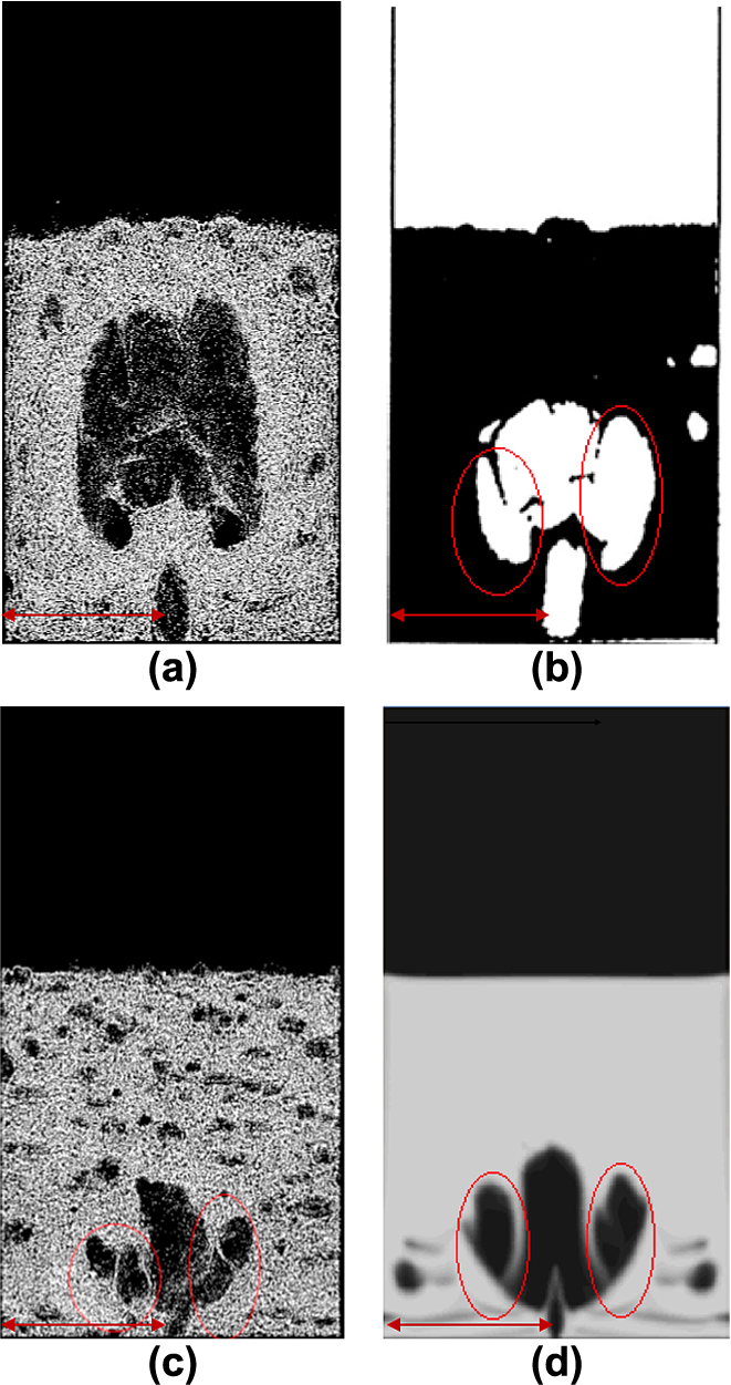
Formation of single bubble in a thin fluidized bed after 0.4 s; (left to tight) (a) Solid pressure model (b) Experimental (Kuipers, 1990), (c) Complete solid stress (d) Euler-Euler model. Scale bar is 0.025 m.

This can be explained by the fact that the shear forces will restrict the single bubble from further expansion and new bubbles will grow out of the original bubble. Therefore, the last two terms were added to the solid stress equation (5) to consider the shear stress generated by granular flow. As it can be seen in Fig. 2(c), the bubble is broken into three parts which shows the effect of shear stresses on the bubble breakage. Moreover, a Eulerian-Eulerian simulation was performed using the same conditions and drag model as a control. The results showed the same trend of bubble breakage as the DDPM model with the consideration of a solid stress. However, the bubble breakage happens quickly in the bed compared to the experimental results, which can be related to the discontinuity in the drag model. After studying the effect of solid stress on formation and expansion of a single bubble, a freely bubbling fluidized bed was simulated. The bubbling fluidized bed works at volume fractions close to packing limit which makes the tangential forces more important.

Fig. 3 shows the snapshots of a freely bubbling bed at the initial conditions using two different collision approaches. As it is shown, the large bubble is formed at the center of the bed as a result of breakage, expansion and coalescence of the bubbles when shear stress is included in the model. On the other hand, the bubbles are formed separately through the whole bed using the solid pressure approach. The number of bubbles and the solid volume fraction in the bubbles for the case with the solid pressure approach are higher. This means bubbles are initially formed but they cannot grow so much because the normal forces are smaller at lower velocities and shear forces are dominant.

Fig. 3

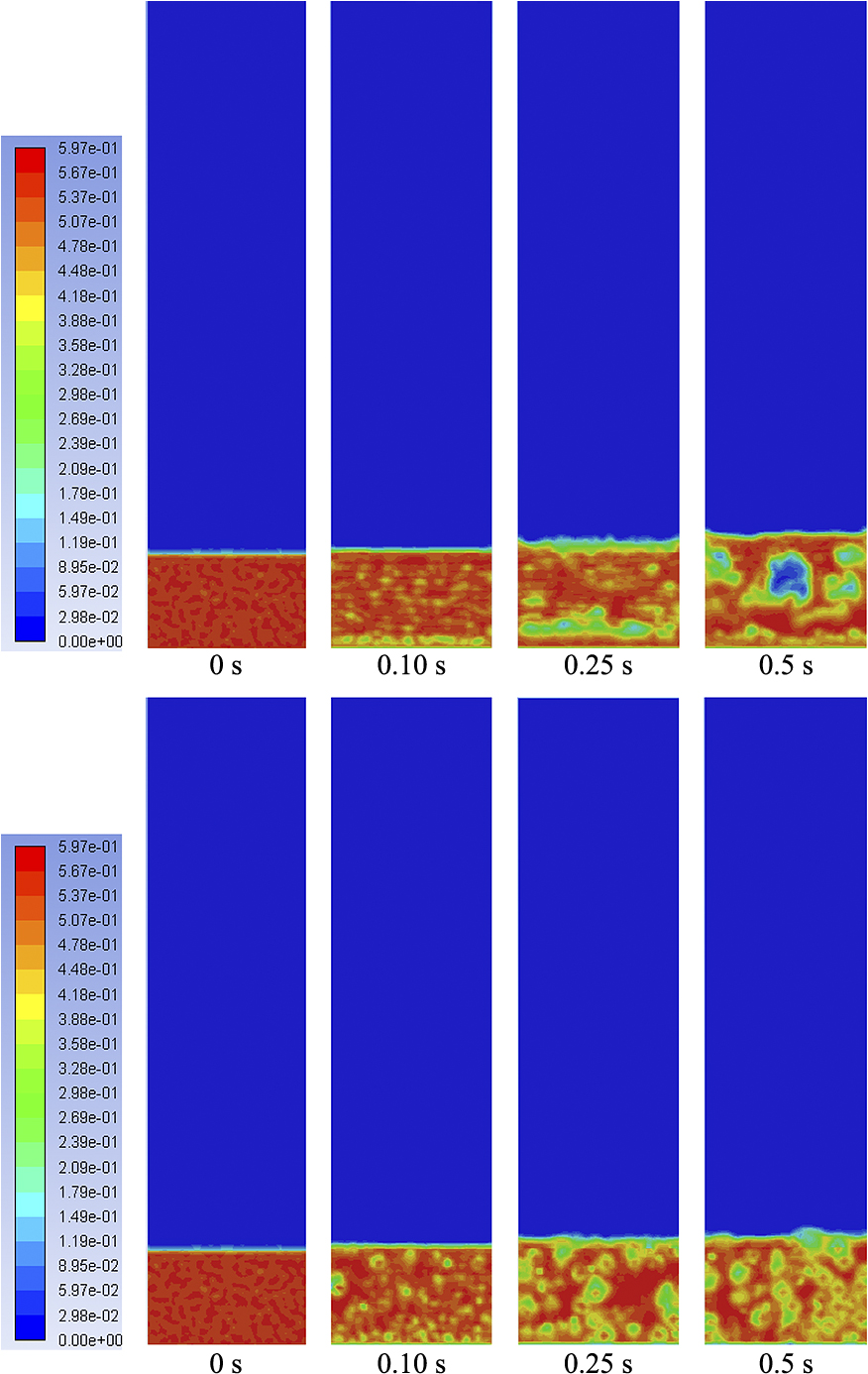
The instantaneous solid volume fraction of freely bubbling bed at the initial condition simulated using complete solid stress (top) and solid pressure (bottom).

On the other hand, after the first generation of bubbles is formed in the case with the solid stress approach, they are attached to each other to form a larger bubble and finally a central bubble passing through the bed is formed. Fig. 4 shows the probability of the formation of bubble at the height of 0.25 m above the bed. As it can be seen, the probability of the formation of bubble is fluctuating through the whole bed for the case that a solid pressure is used to represent the particle interactions. Coalescence and breakage of the bubbles are not observed in this case which confirms the previously reported results in the literature (Liang et al., 2014).

Fig. 4

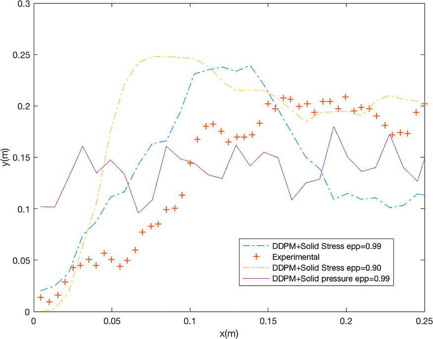
Probability of formation bubbles at 0.25 m above the bed for model predictions and experimental from (Hernández, 2013).

In addition, the performance of the model in prediction of the probability of formation bubbles was evaluated quantitatively using the root-mean-square deviation (RMSD), which is defined as follows:

  

$$RMSD=\sqrt{\frac{1}{N}\sum _{i=1}^N{(Y_i-X_i)}^2}$$(16)

Where X_i and Y_i denote the experimental and predicted values respectively, and N is the number of observations. Also, coefficient of variation was used to calculate the relative discrepancy of the simulations:

  

$$CV=\frac{\sqrt{\frac{1}{N}{\sum }_{i=1}^N{(Y_i-X_i)}^2}}{\sqrt{\frac{1}{N}{\sum }_{i=1}^N{(X_i)}^2}}$$(17)

The calculated discrepancies between experimental and simulation results in the form of RMSD and CV are presented in the Table 2. As it can be seen in the table the model with solid pressure for prediction of particle collisions has several orders of magnitudes (729 %) deviation from the experimental results in prediction of bubble formation probability. The stress model results produce smaller discrepancies (100 and 57.1 %) which is in the same order of magnitude reported using Eulerian models in the literature (Hernández, 2013). The effect of front and back wall friction and the configuration of the distributor holes can be the reasons for current amount of discrepancies between simulation and experimental results.

Table 2 Discrepancy of simulations from experimental results using different collision models.

Quantity	Unit	Solid Stress, epp = 0.90	Solid Stress, epp = 0.99	Solid Pressure, epp = 0.99
RMSD	—	0.0031	0.0018	0.0224
CV	%	100	57.1	729

When the tangential forces are involved in the solid stress in a DDPM model, the probability of the formation of the bubble is in a better agreement with experimental results and the predictions. It means that using a solid pressure to represent the collisions in the freely bubbling fluidized bed will not simulate the bubble pathways through the center of the bed and downward movement of particles. It should be noticed that in freely bubbling beds tangential forces are larger compared to a single bubble bed case formed by high velocity jet.

Fig. 5(a, c, e) shows the contours of the bubble probability and the time averaged solid volume fraction in the bed for the experimental results and predictions. The bubbles are mostly formed in the center and close to the surface of the bed. The model with the solid stress approach was in a good agreement with the trend of experimental results, but the model with a solid pressure overpredicted the formation of bubbles at the bottom of the bed and underpredicts the formation of bubbles close to the surface of the bed. This is because tangential stresses are dominant in the case of bubbling fluidized beds and ignoring these terms would lead to unrealistic predictions in bubble formation which controls the bed hydrodynamics. The discrepancies between the model predictions and experimental results can be related to the non-ideal distribution of the air using a perforated distributor in the experiments. Moreover, the experimental time averaged solid volume fraction is compared with the model predictions in Fig. 5(b, d, f). As it shows, the solids are close to packing limit beside the wall because the bubbles don’t expand and rise in that region and their pathway is through the center of the bed. This is consistent with the well-known downward movements of particles beside the wall which inhabits the rising of bubbles.

Fig. 5

Probability of formation of bubble $\overline{B}$ (left) and Solid volume fraction (right) (a & b) Experimental (Hernández, 2013) (c & d) Model with solid pressure (e & f) Model with solid stress.

One of the parameters in a solid stress is the coefficient of restitution that can be determined by the elasticity of the particles. Fig. 6 shows the effect of this parameter on hydrodynamics of bubbles. The particle volume fraction inside the bubbles was increased from 5 % to 30 % when coefficient of restitution was increased from 0.90 to 0.99. It means that fewer bubbles are formed when the coefficient of restitution is increased. As shown in Fig. 6, the formation of wake under the bubbles in the bubbling fluidized bed confirms the similar shapes of bubbles reported in the literature. High velocity of particles under a rising bubble creates low pressure under the bubble which leads to the deformation of the tracking bubbles. This is the main mechanism in formation of bubble path in bubbling fluidized beds.

Fig. 6

DPM volume fraction as function of coefficient of restitution.

The coefficient of restitution can be used as a controlling parameter to predict the fluidization of sticky particles using a DDPM model. It means that more segregation can happen between gas and solid phase when the coefficient of restitution is decreased.

5. Conclusion

Single bubble and freely bubbling fluidized beds were used to compare the ability of a modified hybrid Eulerian Lagrangian model for the prediction of single and multiple bubble behavior. Dense Discrete Phase Model coupled with kinetic theory of granular flows was used to build the model. Collision between particles were modeled by gradient of solid stress calculated from Eulerian grid and KTGF. The results showed that the predictions of bubbling hydrodynamics using hybrid Lagrangian Eulerian methods were improved using a solid stress compare to solid pressure-based model. It was found that eliminating the tangential forces in current state of the hybrid Lagrangian Eulerian method lead to discrepancies in predictions.

The results showed that a dense discrete phase model coupled with kinetic theory of a granular flow is a reliable approach if the solid stress is used in its complete form. It was shown that using a solid normal pressure instead of a solid stress will lead to the formation of round bubbles in a normal force dominant region in a fluidization bed. However, the formation of bubbles was underpredicted in the shear force dominant region. The probability of the formation of bubbles was deviating from experiments using the solid pressure approach in a freely bubbling fluidized bed.

Acknowledgements

This work was partially supported by the United States NSF-CREST Center for Bioenergy [Award No. HRD-1242152] and the United States Department of Energy [Award No. EE0003138].

Authors’ Short Biographies

Abolhasan Hashemisohi

Abolhasan Hashemisohi is a PhD candidate in Computational Science and Engineering at North Carolina Agricultural and Technical State University (NC A&T) under supervision of Dr. Lijun Wang and Dr. Abolghasem Shahbazi. He completed his Bachelor of science in Chemical Engineering (2009) University of Arak, Iran. He received his Master degree in Chemical Engineering with focus on Thermodynamics and Kinetics (2012). His research interests range from reaction engineering, heterogenous catalysis to simulation of fluidized bed reactors using computational fluid dynamics. He has been working on modelling and improvement of biomass gasification in fluidized beds since 2014 at NSF CREST Bioenergy Center.

Lijun Wang

Dr. Lijun Wang is a professor of biological engineering at NC A&T State University. Dr. Wang has 25 years of experience as a process engineer in advancing bioprocessing and biofuel research. He focuses his efforts on converting biomass into biofuels and biobased products and improving energy efficiency in processing facilities. Wang is one of three thrust leaders of the interdisciplinary NSF CREST Bioenergy Center to lead the biomass gasification research. Dr. Wang is a licensed professional engineer in North Carolina and Nebraska and certified energy manager with the Association of Energy Engineers. He is a member of the American Institute of Chemical Engineers, and American Society of Agricultural and Biological Engineers.

Abolghasem Shahbazi

Abolghasem Shahbazi is a professor of Biological Engineering and the administrative director of CREST Center for Bioenergy. Dr. Shahbazi has over twenty-five years of experience with bioenergy and bioprocess engineering research. He has authored/co-authored more than 90 peer reviewed research publications and was the recipient of an interdisciplinary research award in 2014. He is a member of American Society for Agricultural and Biological Engineers. He has served as a member of Technical Advisory Committee for Biomass Research and Development Initiative for US Departments of Energy and Agriculture from April 2012 until December 2017. Dr. Shahbazi served as a co-chair of symposium on thermal and catalytic sciences for biofuels and bio-based products which was held at the Friday Center, UNC Chapel Hill, NC, November 2–4, 2016.

References

•  Benyahia  S.,  Galvin  J.E., Estimation of numerical errors related to some basic assumptions in discrete particle methods, Industrial & Engineering Chemistry Research, 49 (2010) 10588–10605. DOI: 10.1021/ie100662z
•  Cloete  S.,  Johansen  S.T.,  Amini  S., Performance evaluation of a complete Lagrangian KTGF approach for dilute granular flow modelling, Powder Technology, 226 (2012) 43–52. DOI: 10.1016/j.powtec.2012.04.010
•  Cocco  R.,  Issangya  A.,  Karri  S.B.R.,  Freeman  T.,  Jaeger  H.M.,  Knowlton  T.M., Small-scale particle interactions are having significant effects on global fluidized bed behavior, KONA Powder and Particle Journal, 34 (2017) 155–167. DOI: 10.14356/kona.2017021
•  Cocco  R.,  Fullmer  W.D.,  Liu  P.,  Hrenya  C., CFD-DEM: Modeling the small to understand the large, Chemical Engineering Progress, 113 (2017) 38–45.
•  Davidson  J.F.,  Harrison  D., The behaviour of a continuously bubbling fluidised bed, Chemical Engineering Science, 21 (1966) 731–738. DOI: 10.1016/0009-2509(66)87001-X
•  Ding  J.,  Gidaspow  D., A bubbling fluidization model using kinetic theory of granular flow, AIChE Journal, 36 (1990) 523–538. DOI: 10.1002/aic.690360404
•  Fotovat  F.,  Abbasi  A.,  Spiteri  R.J.,  de Lasa  H.,  Chaouki  J., A CPFD model for a bubbly biomass-sand fluidized bed, Powder Technology, 275 (2015) 39–50. DOI: 10.1016/j.powtec.2015.01.005
•  Gidaspow  D., Multiphase Flow and Fluidization: Continuum and Kinetic Theory Descriptions, 1 edition, Academic Press, Boston, 1994.
•  Grace  J.R., High-velocity fluidized bed reactors, Chemical Engineering Science, 45 (1990) 1953–1966.
•  Hashemi Sohi  A.,  Eslami  A.,  Sheikhi  A.,  Sotudeh-Gharebagh  R., Sequential-based process modeling of natural gas combustion in a fluidized bed reactor, Energy & Fuels, 26 (2012) 2058–2067. DOI: 10.1021/ef300204j
•  Hernández Jiménez  F., Numerical and experimental investigations on pseudo-2D gas fluidized beds, Dissertation at the University Carlos III of Madrid, 2013.
•  Hoomans  B.P.B.,  Kuipers  J.A.M.,  Briels  W.J.,  van Swaaij  W. P.M., Discrete particle simulation of bubble and slug formation in a two-dimensional gas-fluidised bed: A hard-sphere approach, Chemical Engineering Science, 51 (1996) 99–118. DOI: 10.1016/0009-2509(95)00271-5
•  Igci  Y.,  Andrews IV  A.T.,  Sundaresan  S.,  Pannala  S., &  O’Brien  T., Filtered two-fluid models for fluidized gas-particle suspensions, AIChE Journal, 54 (2008) 1431–1448. DOI: 10.1002/aic.11481
•  Kuipers  J.A.M., A two-fluid micro balance model for fluidized beds, Dissertation at the University of Twente, 1990.
•  Kunii  D.,  Levenspiel  O., Fluidization Engineering, Butterworth-Heinemann, 1991.
•  Leonard  B.,  Mokhtari  S., ULTRA-SHARP nonoscillatory convection schemes for high-speed steady multidimensional flow, NASA Technical Memorandum, (1990) 19900012254 (pp50).
•  Liang  Y.,  Zhang  Y.,  Li  T.,  Lu  C., A critical validation study on CPFD model in simulating gas – solid bubbling fluidized beds, Powder Technology, 263 (2014) 121–134. DOI: 10.1016/j.powtec.2014.05.003
•  Lu  L.,  Gopalan  B.,  Benyahia  S., Assessment of different discrete particle methods ability to predict gas-particle flow in a small-scale fluidized bed, Industrial and Engineering Chemistry Research, 56 (2017) 7865–7876. DOI: 10.1021/acs.iecr.7b01862
•  Lun  C.K.K.,  Savage  S.B.,  Jeffrey  D.J.,  Chepurniy  N., Kinetic theories for granular flow: Inelastic particles in Couette flow and slightly inelastic particles in a general flowfield, Journal of Fluid Mechanics, 140 (1984) 223–256. DOI: 10.1017/S0022112084000586
•  Norouzi  H.R.,  Zarghami  R.,  Mostoufi  N., New hybrid CPU-GPU solver for CFD-DEM simulation of fluidized beds, Powder Technology, 316 (2017) 233–244. DOI: 10.1016/j.powtec.2016.11.061
•  Patankar  S., Numerical heat transfer and fluid flow, CRC Press, 1980. ISBN 9780891165224 - CAT# RT5223.
•  Popoff  B.,  Braun  M., A lagrangian approach to dense particulate flows, Proceedings of the ICMF 2007, 6th International Conference on Multiphase Flow, (2007) 11.
•  Radl  S.,  Sundaresan  S., A drag model for filtered Euler-Lagrange simulations of clustered gas-particle suspensions, Chemical Engineering Science, 117 (2014) 416–425. DOI: 10.1016/j.ces.2014.07.011
•  Singhal  A.,  Cloete  S.,  Radl  S.,  Quinta-Ferreira  R.,  Amini  S., Comparison of particle-resolved direct numerical simulation and 1D modelling of catalytic reactions in a packed bed, 12th International Conference on CFD in the Oil & Gas, Metallurgical and Process Industries (CFD2017), (2017).
•  Snider  D.M., Three fundamental granular flow experiments and CPFD predictions, Powder Technology, 176 (2007) 36–46. DOI: 10.1016/j.powtec.2007.01.032
•  Tsuji  Y.,  Kawaguchi  T., &  Tanaka  T., Discrete particle simulation of two-dimensional fluidized bed, Powder Technology, 77 (1993) 79–87. DOI: 10.1016/0032-5910(93)85010-7