On the Similarity of Austin Model and Kotake–Kanda Model and Implications for Tumbling Ball Mill Scale-Up

Abstract

The aim of this theoretical investigation is to seek any similarities between the Austin model and the Kotake–Kanda (KK) model for the specific breakage rate function in the population balance model (PBM) used for tumbling ball milling and assess feasibility of the KK model for scale-up. For both models, the limiting behavior for small particle size-to-ball size ratio and the extremum behavior for a given ball size are described by “power-law.” Motivated by this similarity, specific breakage rate data were generated using the Austin model parameters obtained from the lab-scale ball milling of coal and fitted by the KK model successfully. Then, using the Austin’s scale-up methodology, the specific breakage rate was scaled-up numerically for various mill diameter scale-up ratios and ball sizes of 30–49 mm and coal particle sizes of 0.0106–30 mm. PBM simulations suggest that the KK model predicts identical evolution of the particle size distribution to that by the Austin model prior to scale-up. Upon scale-up, the differences are relatively small. Hence, modification of the exponents in the Austin’s scale-up methodology is not warranted for scale-up with the KK model. Overall, this study has established the similarity of both models for simulation and scale-up.

1. Introduction

Tumbling ball mills have been commonly used in a multitude of industries, especially the minerals industry (Austin et al., 1984). Population balance modeling (PBM) enables engineers to simulate, design, control, and scale-up various particulate processes (Randolph and Larson, 1988; King, 2001), including the tumbling ball milling (Austin et al., 1984; Prasher, 1987). The size-discrete, time-continuous form of the PBM (Sedlatschek and Bass, 1953) for a well-mixed ball mill operating in batch mode is expressed as

  

$$\frac{\text{d}{M}_i}{\text{d}t}=-S_i{M}_i+\sum _{j=1}^{i-1}{b}_{ij}{S}_j{M}_j\hspace{0.17em}\text{with\hspace{0.17em}}{M}_i(0)=M_{i,\text{ini}}$$(1)

where i and j are the size-class indices running up to N_s (sink size class). Here, t, M_i, S_i, and b_ij represent time, mass fraction, specific breakage rate parameter, and breakage distribution parameter, respectively. Eqn. (1) also assumes first-order (linear) breakage kinetics and has been successfully used for simulating the milling of a wide variety of materials in different types of mills (Austin et al., 1984; King, 2001). Readers are referred to Bilgili and Scarlett (2005) and Capece et al. (2011) for an extensive review and a PBM framework for treatment of nonlinear breakage kinetics.

It has been experimentally well-established that S_i varies significantly with design and operating conditions for a given material to be ground in ball mills (Austin et al., 1984). The celebrated Austin model describes how S_i varies as a function of particle size x_i:

  

$$S_i=a_{\text{T}}{x}_i^{\alpha }\frac{1}{1+{(x_i/{\mu }_{\text{T}})}^{\mathit{\Lambda }}}$$(2)

Here, a_T and μ_T are parameters that strongly depend on the milling conditions, the material, and the ball size, whereas α and Λ are positive constants that largely depend on the properties of the material. Austin et al. (2007) assert that Λ can be satisfactorily taken as 3 for most materials. Some researchers assumed Λ = 3 (e.g., Bwalya et al., 2014) or fitted Λ to find it within ±10 % of this value (Rogers et al., 1986; Petrakis et al., 2017); yet others found notably different values: 4.74 (Chimwani et al., 2013) and 2.4 (Shahcheraghi et al., 2019). Traditionally, these parameters have been estimated via either direct calculation of S_i by one-size-fraction method (Austin and Bhatia, 1971–72) or the optimization-based back-calculation method (Klimpel and Austin, 1977) using experimental data from small or pilot scale ball mills. As balls are an integral element of the ball mill design, the impact of ball size d_B on a_T and μ_T has been extensively studied (Austin et al., 1976a; 1984; Katubilwa and Moys, 2009). The Austin model can be recast into the following form with explicit ball size dependence (e.g., Katubilwa and Moys, 2009, with slight differences in formalism):

  

$$S_i=a_0{x}_i^{\alpha }\frac{{\left(d_{\text{B},0}/d_{\text{B}}\right)}^{\xi }}{1+{\left[x_i/\left({\mu }_0{\left(d_{\text{B}}/d_{\text{B},0}\right)}^{\eta }\right)\right]}^{\mathit{\Lambda }}}$$(3)

where a₀ and μ₀ are the values of a_T and μ_T for specific ball size d_B,0 in the small/pilot scale batch milling experiments, while η and ξ are constant ball-size exponents. For a mixture of balls, the specific breakage rate is calculated from the mass fraction of each ball size M_{B, p} and its corresponding S_{i, p} as follows:

  

$$\overline{S_i}=\sum _{p=1}^P{M}_{\text{B},p}{S}_{i,p}$$(4)

Scale-up of tumbling ball mills from small-scale batch mills to industrial scale mills has been successfully implemented within the context of PBM (Austin et al., 1984; Yildirim et al., 1999; Chimwani et al., 2014; De Oliveira and Tavares, 2018). In this approach, empirical equations are used for determining the dependence of the breakage parameters on ball/mill dimensions and operating variables at the lab-scale and large-scale industrial mills. It is important to emphasize that scale-up from a batch mill to continuous large-scale mills entails modification of the breakage parameters (S_i and b_ij) as well as consideration of the residence time distribution and internal–external classification in the continuous mills (Herbst and Fuerstenau, 1980; Austin et al., 1984; Rogers and Austin, 1984; De Oliveira and Tavares 2018). Although each one of these aspects is important, this study focuses on the scale-up of the specific breakage rate S_i.

Upon scale-up, S_i is known to change significantly, whereas b_ij or its cumulative counterpart B_ij is generally assumed to remain invariant unless ball size/type changes significantly (Herbst and Fuerstenau, 1980; Austin et al., 1984). In accounting for scale-up related changes, the Austin’s methodology scales-up S_i in Eqn. (2) via correction factors K₁–K₅ that depend on the design parameters of the dry ball mill and operating conditions as follows:

  

$${S_i}^{*}=a_{\text{T}}{x}_i^{\alpha }\frac{1}{1+{[x_i/(K_1{\mu }_{\text{T}})]}^{\mathit{\Lambda }}}{K}_2{K}_3{K}_4{K}_5$$(5)

  

$$K_1={\left(\frac{D}{D_{\text{T}}}\right)}^{N_2}{\left(\frac{d_{\text{B}}}{d_{\text{B},\text{T}}}\right)}^{N_3},K_2={\left(\frac{d_{\text{B},\text{T}}}{d_{\text{B}}}\right)}^{N_0}$$(6)

  

$$K_3=\{\begin{array}{ll}{\left(\frac{D}{D_{\text{T}}}\right)}^{N_1}\hfill & \text{if\hspace{0.17em}}D\le 3.81\hspace{0.17em}\text{m}\hfill \\ {\left(\frac{3.81}{D_{\text{T}}}\right)}^{N_1}{\left(\frac{D}{3.81}\right)}^{N_1-N_4}\hfill & \text{if\hspace{0.17em}}D>3.81\hspace{0.17em}\text{m}\hfill \end{array}$$(7)

  

$$K_4=\frac{1+6.6J_{\text{T}}^{2.3}}{1+6.6J^{2.3}}\text{exp\hspace{0.17em}}[-1.2(U-U_{\text{T}})]$$(8)

  

$$K_5=\left(\frac{{\varphi }_{\text{C}}-0.1}{{\varphi }_{\text{C},\text{T}}-0.1}\right)\left\{\frac{1+\text{exp\hspace{0.17em}}[15.7({\varphi }_{\text{C},\text{T}}-0.94)]}{1+\text{exp\hspace{0.17em}}[15.7({\varphi }_{\text{C}}-0.94)]}\right\}$$(9)

where D, J, U, and ϕ_C denote the mill diameter, the fractional mill filling by the balls, the void filling fraction, and the fraction of actual rotation speed compared to the critical speed N_C. The subscript T refers to the parameters used in the small-scale batch test, which are used to fit the model parameters in Eqns. (2) and (3). Typical scale-up exponents are N₀ = 1, N₁ = 0.5, N₂ = 0.2, N₃ = 2, and N₄ = 0.2 (Austin et al., 1984). However, other values of N₃ were also used such as 1 (Yildirim, 1999) and 1.2 (Austin et al., 2007). One should note that N₀ and N₃ should be taken as ξ and η of Eqn. (3), respectively, from a study on the ball size impact on S_i at the test (T) scale, which is a preferred approach (Mulenga, 2017).

While the Austin model in Eqn. (2) or (3) has been the most widely used kinetic model for ball milling, Kotake et al. (2002, 2004) developed the following kinetic model for the breakage of narrowly sized feed with size x_f:

  

$$S_1=C_1{d}_{\text{B}}^m{x}_{\text{f}}^{\alpha }\hspace{0.17em}\text{exp\hspace{0.17em}}\left(-\frac{C_2{x}_{\text{f}}}{d_{\text{B}}^n}\right)$$(10)

which we briefly refer to as the KK (Kotake–Kanda) model for the sake of simplicity. The parameters C₁ and C₂ strongly depend on the milling conditions and material properties, whereas α is a positive constant that largely depends on the properties of the material; m and n are material-dependent, ball size exponents. Kotake et al. (2002, 2004) and Deniz (2003) demonstrated the fitting capability of this model for ball milling of a multitude of minerals. The KK model, Eqn. (10), is appealing as it has 5 parameters as opposed to the Austin model with 6 parameters, when ball sizes are explicitly considered. The milling studies, where the back-calculation approach involved more than a few breakage parameters to be estimated, have shown that the accuracy decreases as the number of parameters to be estimated increases (Klimpel and Austin, 1977; Kwon and Cho, 2021). However, to the best knowledge of the author, the KK model has not been used for the PBM simulation of ball milling of a natural feed with a wide size particle size distribution (PSD), and no scale-up has been performed using it. More importantly, the KK model has never been compared to the Austin model.

The present theoretical investigation seeks answers to the following questions: (i) Are there any similarities between the Austin model and the KK model despite their different mathematical forms? (ii) Is the Austin’s scale-up methodology (scale-up correction factors) applicable to the KK model? (iii) Do these models predict similar time-wise evolution of PSD in ball mills before and after scale-up? To be able to answer these questions, we first generated synthetic specific breakage rate data using the Austin model, whose parameters were obtained from the lab-scale ball milling of coal. Next, this data was fitted by the KK model to determine its parameters. Then, using the Austin’s scale-up methodology, the specific breakage rate was scaled-up numerically (virtual scale-up) using both models for various mill diameter scale-up ratios D/D_T from 4 to 10, ball sizes d_B of 30–49 mm, and coal particle sizes x_i of 0.0106–30 mm. PBM simulations assumed plug flow and invariance of b_ij in the large-scale mills and incorporated the scaled-up S_i values. The PBM simulations were performed for the small-scale mill and the large-scale mills. Upon scale-up, we find that the differences in both models’ predictions are relatively small. Instead of just using N₁ = 0.5 and N₂ = 0.2 for the virtual scale-up with the KK model, which is based on the Austin’s scale-up methodology, we also fitted these exponents to the S_i values generated by the Austin kinetic model, keeping the other scale-up exponents the same. Comparison of the PSD evolution prediction by the KK model (with/without modified N₁ and N₂) and the Austin model will allow us to find the answers to the above-mentioned questions.

2. Theoretical approach

2.1 Experimental data and model calibration

The KK model can be cast into the following form, which is valid for any arbitrary particle size x_i

  

$$S_i=C_1{d}_{\text{B}}^m{x}_i^{\alpha }\hspace{0.17em}\text{exp\hspace{0.17em}}\left(-\frac{C_2{x}_i}{d_{\text{B}}^n}\right)$$(11)

Note that both Eqns. (3) and (11) are explicit in d_B and x_i, which enables us to discern any similarities or differences between the two models by analyzing the limiting behavior for small particle size-to-ball size ratio and the extremum behavior for a given ball size. To demonstrate that the KK model can predict the same S_i as that predicted by the Austin model, we need to have S_i parameters from an experimental data set on batch ball milling. Hence, we considered the experimental work on the batch ball milling of a South African coal (Katubilwa and Moys, 2009). They fitted and/or set the Austin model parameters as follows: a₀ = 0.48 mm^−0.81∙min⁻¹, μ₀ = 19.27 mm, d_B,0 = 38.8 mm, α = 0.81, Λ = 3, ξ = 1, and η = 1.96. Using this set of parameters, a synthetic data set for S_i was generated by the Austin model using Eqn. (3) for ball sizes of 30–49 mm with increments of 1 mm and coal particle sizes of 0.0106–30 mm with a geometric progression ratio of 2^1/13. As the purpose of this study is to examine theoretical similarity of the KK model to the Austin model, we did not fit the KK model to the experimental data directly, but to the synthetic S_i data generated by the Austin model to minimize any bias. Both models have been shown to fit various ball milling data successfully in the milling literature; the question we seek to answer here is not how well they can fit specific experimental data. Therefore, the parameters of the KK model, Eqn. (11), were estimated by minimizing the sum-of-squared residuals between the KK model prediction and the synthetic data generated by the Austin model for the South African coal. In comparison to no transform and logarithmic transform, a square-root transform of the response (S_i) led to the best overall fitting and simulation results when the KK model with the estimated parameters were compared with the Austin model. Hence, only the KK model parameters obtained by fitting after the square-root transform of the response (S_i) are presented. The optimization was performed via the Marquardt–Levenberg method in Minitab version 21.1.

2.2 Virtual scale-up

A virtual scale-up of the specific breakage rate S_i was performed from the small-scale batch mill to the large-scale continuous ball mills. Using the Austin’s scale-up methodology, the specific breakage rate S_i obtained experimentally for the Austin model (Katubilwa and Moys, 2009) and the KK model with the estimated parameters (refer to Section 2.1) were scaled-up numerically for various mill diameter scale-up ratios D/D_T from 4 to 10, ball sizes d_B of 30–49 mm, and coal particle sizes x_i of 0.0106–30 mm. For simplicity, K₄ and K₅ are set to 1 in this study for the scale-up with both models regardless of any particular values of J, U, and ϕ_c values because K₄ and K₅ are independent of d_B/d_T ≡ d_B/d_B0 and D/D_T, which were varied in this study. Hence, the scaled-up S_i, i.e., S_i^*, was calculated by

  

$${S_i}^{*}=a_0{x}_i^{\alpha }\frac{{(d_{\text{B},0}/d_{\text{B}})}^{\xi }\hspace{0.17em}{K}_3}{1+{\left[\frac{x_i}{{\mu }_0{(D/D_{\text{T}})}^{N_2}{(d_{\text{B}}/d_{\text{B},0})}^{\eta }}\right]}^{\mathit{\Lambda }}}$$(12)

  

$${S_i}^{*}=C_1{d}_{\text{B}}^m{x}_i^{\alpha }\hspace{0.17em}\text{exp\hspace{0.17em}}\left(-\frac{C_2{x}_i}{{(D/D_{\text{T}})}^{N_2}\hspace{0.17em}{d}_{\text{B}}^n}\right)\hspace{0.17em}{K}_3$$(13)

The above equations incorporate K₁, K₂, and K₃ directly, which depend on d_B/d_B0 and D/D_T. First, Eqn. (12) was used to generate the S_i^* by the Austin model for all scale-up scenarios with various d_B/d_B0 and D/D_T. These scaled-up data were taken as the “synthetic scale-up data” against which the scale-up with the KK model was compared. Then, two different virtual scale-up approaches for the KK model were used. In the first approach, the standard scale-up exponents of the Austin’s scale-up methodology, i.e., N₁ = 0.5 and N₂ = 0.2, along with N₄ = 0.2 were used in Eqn. (13) to predict the S_i^*. However, as there is no prior scale-up study with the KK model, one cannot assume that the Austin’s scale-up exponents N₁ and N₂ are directly applicable for use in Eqn. (13). Hence, in the second approach, we fitted S_i^* values generated by Eqn. (12) for each D/D_T from 4 to 10 and ball sizes d_B of 30–49 mm using Eqn. (13) and minimizing the following standard error SE:

  

$$SE=\sqrt{\frac{{\sum }_{i=1}^N{\left(\sqrt{S_{\text{Austin},i}^{*}}-\sqrt{S_{\text{KK},i}^{*}}\right)}^2}{N-N_{\text{p}}}}$$(14)

which allowed us to estimate N₁ and N₂. An additional fit was performed to minimize SE for all D/D_T cases simultaneously. Here, N and N_p refer to the total number of data points and parameters estimated, respectively. Then, these simultaneously estimated values of N₁ and N₂ were used to predict S_i^* for each scale-up scenario separately.

2.3 PBM simulations

The scale-up from a small batch mill or a pilot-scale mill to a large-scale industrial continuous mill is a complex endeavor, entailing considerations of the residence time distribution (RTD), internal classification, and external classification in the continuous mill circuits (Herbst and Fuerstenau, 1980; Austin et al., 1984; Rogers and Austin, 1984; De Oliveira and Tavares, 2018) besides scale-up of the specific breakage rate. However, any consideration of these factors in the scale-up process would complicate the analysis to discern the differences between the Austin model and KK model in the scale-up of S_i. Hence, we followed the simplest approach for the modeling of an open-circuit continuous mill by assuming plug flow behavior and disregarding any internal classification in the mill. This simple approach purposefully isolates the problem of “breakage kinetics” in scale-up and allows us to focus on the discrimination of the KK model from the Austin model within the context of simulation and scale-up. The plug-flow is a viable assumption for some industrial scale ball mills (Austin, 1973). For example, a 10 tanks-in-series model represented the RTD data for a large-scale cement ball mill (Austin et al., 1975). The plug-flow assumption was also adopted by other researchers in the ball mill scale-up (Chimwani et al., 2014). Developing a sophisticated PBM for a continuous ball mill circuit with internal–external classification is not within the scope of this study.

Note that Eqn. (1) is applicable to mills operating in batch mode as well as plug-flow continuous mode. One can replace time t with contact time t* = y/u for any axial position y in the mill with u denoting the average axial velocity of the particles: u = L/τ = LF/M_h, where τ, L, F, and M_h stand for the space-time (the average residence time), length of the mill, inlet mass flow rate, and mass hold-up at steady state, respectively. So, after replacing t with t*, one can solve the set of ordinary differential equations (ODEs) in Eqn. (1) with the initial condition M_i(0) = M_i,ini, with M_i,ini representing the feed PSD, and predict the steady-state PSD at t* = τ. Henceforth, although we use the above formalism, for the sake of simplicity, we will still denote time as t in the results, but keeping in mind, t represents retention time in the batch mill and contact (residence) time in the plug-flow continuous mill at the steady state.

In the PBM simulations, we used the S_i values in Section 2.1 for the small-scale batch mill simulations and S_i^* values, as described in Section 2.2, for the continuous milling. The following cumulative breakage distribution parameters B_ij were taken from Katubilwa et al. (2011) about the same South African coal for which S_i parameters were reported in Section 2.1:

  

$$B_{ij}=\varphi {(x_{i-1}/x_j)}^{\gamma }+(1-\varphi ){(x_{i-1}/x_j)}^{\beta }$$(15)

Here, 0 < ϕ < 1 is a breakage constant, and γ and β are breakage exponents. For the South African coal, ϕ, γ, and β were reported to be 0.51, 0.53, and 3.2, respectively. It is well-known that these parameters are largely material dependent, and are relatively insensitive to the milling conditions, except the ball size (Austin et al., 1984; Prasher, 1987; King, 2001). In a more elaborate model, one could incorporate the impact of ball size on B_ij by making γ dependent on the ball size (Austin et al., 2007). In the present simulations and scale-up, we assumed that B_ij remain invariant to ball size and scale-up, similar to what Chimwani et al. (2014) implemented. Using the B_ij values from Eqn. (15), we calculated b_ij via b_ij = B_ij − B_i+1j.

The initial PSD for the small batch mill simulation and the feed PSD for the continuous mill simulation were taken the same: a Gaussian PSD with a mean size of 20 mm and a standard deviation of 2 mm. The Gaussian PSD was generated using the function “normpdf” in MATLAB^TM version 9.11. Considering the time scale of the batch milling experiments (Katubilwa and Moys, 2009), we simulated 0.5, 1, 2, 4, and 8 min of milling time (or residence time). Another rationale for the selection of 8 min is the following: power-station boilers usually demand 60–70 % of coal particles below 75 μm (Prasher, 1987). Our exploratory simulations suggest 8 min residence time in the large-scale mills could meet this demand approximately. In all PBM simulations, the number of size classes N_s and the geometric progression ratio were set as 320 and 2^1/13, respectively, which yields grid-independent simulation results. The set of ODEs in Eqn. (1) along with either Eqns. (3), (11), and (15) for the small batch mill or Eqns. (12), (13), and (15) for the large-scale continuous mill was solved using the function “ode15s” in MATLAB, which is a highly accurate, variable order–step-size ODE solver (Shampine et al., 2003). The relative error tolerance and the absolute error tolerance were set as 10⁻⁴ and 10⁻⁶, respectively.

3. Results and discussion

3.1 Austin model vs. Kotake–Kanda model

Despite the differences in their mathematical forms, both the Austin model and the KK (Kotake–Kanda) model have similar limiting behavior and extremum behavior. Let us first consider the limiting case of x_i << d_B, for which Eqns. (3) and (11) reduce to

  

$$S_i=a_0{x}_i^{\alpha }\hspace{0.17em}{(d_{\text{B},0}/d_{\text{B}})}^{\xi }\hspace{0.17em}\text{and\hspace{0.17em}}{S}_i=C_1{d}_{\text{B}}^m{x}_i^{\alpha }$$(16)

respectively, because the dominator of Eqn. (3) and exponential term in Eqn. (11) approach 1. Clearly, both models provide power-law dependence of S_i on x_i and d_B in this limit. Note that x_i << d_B has not been strictly defined and x_i/d_B < O(10⁻²) is reasonable for this limiting behavior. To prevent a possible confusion, we assert that this limiting behavior is not a practically irrelevant asymptotic limit. As demonstrated by Austin et al. (1976b) and De Oliveira and Tavares (2018), the whole milling kinetics could be governed by this limiting behavior if the feed or initial size is much smaller than the ball sizes used. The KK model can be made equivalent to the Austin model by imposing

  

$$C_1=a_0{d}_{\text{B},0}^{\delta }\hspace{0.17em}\text{and\hspace{0.17em}}m=-\xi$$(17)

as well as the sameness of α in both equations in terms of the limiting behavior.

Let us now consider the extremum behavior of S_i by setting dS/dx = 0 after taking the equivalent particle size-continuous forms of Eqns. (3) and (11). This analysis yields the particle size x_m at which S_i is at a maximum and has the following S_m:

  

$$x_{\text{m}}={\mu }_0\hspace{0.17em}{[\alpha /(\mathit{\Lambda }-\alpha )]}^{\frac{1}{\mathit{\Lambda }}}\hspace{0.17em}{(d_{\text{B}}/d_{\text{B},0})}^{\eta }\hspace{0.17em}\text{with\hspace{0.17em}}\mathit{\Lambda }>\alpha$$(18)

  

$$S_{\text{m}}=a_0{\mu }_0^{\alpha }\hspace{0.17em}{[\alpha /(\mathit{\Lambda }-\alpha )]}^{\frac{\alpha }{\mathit{\Lambda }}}\left(1-\frac{\alpha }{\mathit{\Lambda }}\right){\left(\frac{d_{\text{B}}}{d_{\text{B},0}}\right)}^{\alpha \eta -\xi }$$(19)

  

$$x_{\text{m}}=(\alpha /C_2)d_{\text{B}}^n$$(20)

  

$$S_{\text{m}}=C_1{\text{e}}^{-\alpha }{(\alpha /C_2)}^{\alpha }\hspace{0.17em}{d}_{\text{B}}^{\alpha n+m}$$(21)

for the Austin model and the KK model, respectively. Similar to the limiting behavior, both models predict a power-law dependence of x_m and S_m on d_B. However, the exponents for the limiting behavior and the extremum behavior are different. One can make both models equivalent in terms of the extremum behavior alone, i.e., identical x_m and S_m, by setting the KK parameters as

  

$$C_1=a_0{\text{e}}^{\alpha }\hspace{0.17em}(1-\alpha /\mathit{\Lambda })d_{\text{B},0}^{\xi }$$(22)

  

$$C_2=(\alpha /{\mu }_0){(\mathit{\Lambda }/\alpha -1)}^{1/\mathit{\Lambda }}\hspace{0.17em}{d}_{\text{B},0}^{\eta }$$(23)

n = η, m = −ξ, and same α in both equations.

An interesting theoretical question arises as to what happens if the equivalence conditions, i.e., either Eqn. (17) for the limiting behavior or Eqns. (22)–(23) for the extremum behavior are imposed on the KK model. We note that the conditions imposed on C₁ are incompatible because e^α(1–α/Λ) = 1 is overly restrictive and cannot be satisfied, except for α = 0, which is untenable. If one imposes the equivalence in terms of the extremum behavior, then C₁ provided by Eqn. (22) will be similar to C₁ provided by Eqn. (17) in terms of the power-law dependence with the same exponent ξ. However, Eqn. (22) will overpredict S_i by a factor of e^α(1–α/Λ) in the limit x_i << d_B. This factor equals 1.641 (64.1 %) for the coal considered in Section 2.1, which is not acceptable.

The upshot of the above theoretical analysis is that the KK model is similar, but not equivalent or identical, to the Austin model in terms of the limiting behavior and the extremum behavior. It is impossible to ensure equivalency of these models in terms of both limiting behavior in the size domain x_i << d_B and the extremum behavior in the neighborhood of x_i = x_m. Owing to the power-law dependence of S_i on x_i and d_B in the size domain x_i << d_B and that of x_m and S_m on d_B, we hypothesize that both models could predict similar S_i while satisfying the limiting behavior and the extremum in some approximate statistical sense. Note that they may differ significantly in the size domain x_i << d_B and near the extremum. This hypothesis can be tested by first fitting the KK model parameters to the S_i generated by the Austin model and then analyzing the resulting S_i profiles as well as these models’ prediction of the temporal evolution of the PSD. To this end, the synthetic S_i data generated by the Austin model, whose parameters were obtained by fitting to the ball milling data on a South African coal (refer to Section 2.1), were fitted by the KK model. The parameters of the KK model are presented in Table 1. The sum-of-squared errors was 4.08 min⁻¹, and the standard error SE of the fit was 3.69 × 10⁻² min^−0.5. The parameters had low standard errors: all below 8 %. Clearly, the KK parameters in Table 1 will not satisfy the requirements of Eqn. (17) and Eqns. (22)–(23), which, respectively, ensure equivalency in terms of the limiting behavior and the extremum behavior. These strict conditions are not required for the models to be similar both qualitatively and quantitatively when experimental errors in determining S_i are considered (see later discussion).

Table 1

The KK model parameters obtained from fitting to the synthetic data generated by the Austin model.

Parameter	Value	Unit	SE (%)
C1	107.5	mm0.494·min−1	5.81
m	−1.444	–	1.10
α	0.9496	–	0.242
C2	370.6	mm1.364	7.30
n	2.364	–	0.876

Fig. 1 presents the specific breakage rate S_i data generated by the Austin model for the South African coal and its fitting by the KK model, which led to the estimated parameters in Table 1. While there are minor deviations, the KK model estimated the S_i profiles and the extremum behavior reasonably well. The KK model exhibited a slightly depressed, shifted peak as compared with the Austin model. Both models predict a cliff or falling off S_i for x_i > x_m, which can be explained by the inability of the balls to nip or capture the particles effectively. In view of Eqn. (16), the values of ξ = 1 and m = −1.444 suggest that the smaller ball sizes are effective for x_i << d_B because for the smaller particles, the number frequency of the collisions with the beads govern the specific breakage rate, which is suggested to be scaled by the inverse of d_B, as signified by ξ = 1 (Austin et al., 1984). Overall, both models’ phenomenological representation of the breakage kinetics appears to be qualitatively and quantitatively similar.

Fig. 1

Size dependence of S_i for various ball sizes: fitting by the KK (Kotake) model to the synthetic data generated by the Austin model.

The location of the extremum points in Fig. 1 are given by x_m–S_m, which depend on the ball size d_B and are obtained via Eqns. (18)–(21) for the Austin model and the KK model, respectively, as follows:

  

$$x_{\text{m}}=1.063\times {10}^{-2}\hspace{0.17em}{d}_{\text{B}}^{1.96}\hspace{0.17em}\text{and\hspace{0.17em}}{S}_{\text{m}}=0.3423d_{\text{B}}^{0.588}$$(24)

  

$$x_{\text{m}}=2.562\times {10}^{-3}\hspace{0.17em}{d}_{\text{B}}^{2.36}\hspace{0.17em}\text{and\hspace{0.17em}}{S}_{\text{m}}=0.1439d_{\text{B}}^{0.801}$$(25)

Fig. 2 depicts the variation of x_m and S_m with d_B based on Eqns. (24) and (25). According to the Austin model, each ball size most effectively breaks a certain particle size. Large balls are the best for breaking coarse particles; small balls are the best for breaking small particles. For example, 46 mm balls are most effective for breaking ~20 mm particles; yet, they are the worst for breaking <~8 mm particles; 30 mm balls are most effective for the latter. Practically, for a feed with wide PSD, the common practice is to use a mixture of different ball sizes (Austin et al., 1984; Prasher, 1987; Katubilwa and Moys, 2009).

Fig. 2

Dependence of S_m and x_m on the ball size: Austin model with Eqn. (24) and the KK model with Eqn. (25).

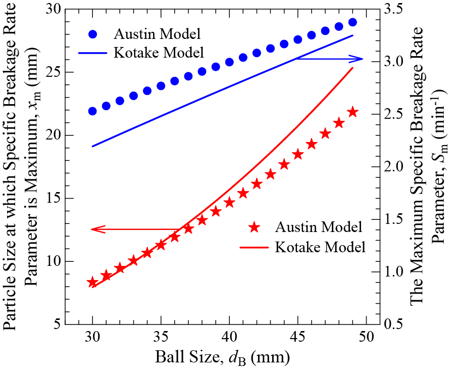
As can be seen from Fig. 2, the KK model provides a similar ball size dependence of S_m and x_m to that by the Austin model although there is some deviation. The mean relative deviation for S_m and x_m were 8.18 % and 7.31 %, respectively, while the maximum relative deviation for S_m and x_m were 13.2 % and 16.1 %, respectively. One interesting trend is that as d_B increased, the S_m deviation of the KK model from the Austin model decreased, while the x_m deviation increased, which counter each other. This observation along with <10 % mean relative deviation overall imply that the deviations may have small impact on the PBM simulation and scale-up results. This is indeed the case, as will be demonstrated next through PBM simulations before and after scale-up.

To develop a deeper understanding of the ball size effects, one must resort to Discrete Element Modeling (DEM) of tumbling ball mills. DEM provides significant fundamental insights and microdynamic information such as collision energies among the balls–particles–mill wall/liners and their frequencies (Tavares, 2017; Rodriguez et al., 2018). In an excellent critical analysis, Rodriguez et al. (2018) pointed out some fundamental learnings from the DEM: (i) Collision energies involving events with only particles (particle–particle and particle–liner) are not sufficiently high to cause breakage of particles and (ii) a fraction of the collisions inside the ball mill do not involve particles; hence, they do not directly contribute to particle breakage. In agreement with the above, the multi-scale PBM–DEM modeling of the experimental tumbling ball mill (Kotake et al., 2002) by Capece et al. (2014) predicted the S_i profile similar to those in Fig. 1. Moreover, their simulations suggest that for a given narrow feed size, an effective ball size that maximizes the specific breakage rate exists. This effective ball size appears to maximize collision frequency with the particles (ball–particle collisions) with sufficiently high impact energy above a minimum threshold impact energy that is particle size-dependent. Such minimum impact energies required to break individual particles under impact loading should be determined experimentally (Tavares and King, 1998; Vogel and Peukert, 2003; Tavares, 2007).

While the analysis of the data in Figs. 1 and 2 suggests that the KK model is similar to the Austin model and they both provide similar S_i, x_m, and S_m, one would argue about the deviations. At this juncture, it is imperative to mention the errors involved in the determination of S_m and x_m. For example, Kotake et al. (2002; 2004) described an averaging procedure to determine S_m and x_m because of the experimental scatter around the maxima. The experimental deviations were certainly greater than the <~10 % S_m and x_m deviations of the KK model from the Austin model observed here. Moreover, the 85 % of the fitted S₁ values by the KK model were within a band of ±20 %, with 15 % of the values outside this band (Kotake et al., 2004); similarly notable deviations can be seen in Deniz (2003). Most importantly, a long-due study (Shahcheraghi et al., 2019) clearly demonstrated that at 95 % confidence level, the experimentally determined S_i parameters of the Austin model had 21.7–34.1 % uncertainty, whereas the B_ij parameters had 7.8–17.8 % uncertainty. Hence, the deviations shown in Figs. 1 and 2 between the Austin model and the KK model would most likely be within the range of experimental uncertainty when the two models are fitted to the same experimental data with repeats. This has never been done in the experimental ball milling literature. In this study, we will confirm the similarity of the two models via PBM simulations next.

A batch ball milling process was simulated by PBM, as described in Section 2.3 to assess if the deviations between the two models’ S_i values could cause significant difference in the simulated time-wise evolution of the PSD. To the best knowledge of the author, this is the first study in which a batch milling process has been simulated by the KK model. Fig. 3 clearly illustrates that despite the S_i deviations illustrated in Fig. 1, the two models simulated the temporal evolution of the PSD almost identically. The maximum deviations in the PSDs estimated by the KK model and the Austin model are within a few percentages. In view of the above discussion and the simulation results, it is clear that the PBM with either the KK model or the Austin model yields a similar temporal evolution of the PSD in a batch mill prior to scale-up. The KK model has one less parameter than the Austin model (5 vs. 6); its use may be advantageous for parameter estimation.

Fig. 3

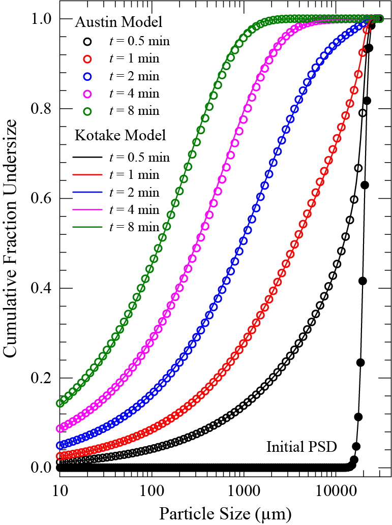
PBM simulation of the time-wise evolution of the cumulative PSD in a batch mill with an initial Gaussian PSD (mean size: 20 mm, SD: 2 mm) and d_B = 38 mm.

3.2 Virtual scale-up with the KK model

Historically, the Austin kinetic model has been used along with Austin’s methodology for ball mill scale-up (Austin et al., 1984). As the KK model has never been used for ball mill scale-up, it is doubtful if it can be integrated with the Austin’s scale-up methodology. In Section 2.2, we developed the scaled-up specific breakage rate parameter S_i^* using this methodology. To the best knowledge of the author, this is the first attempt to use the KK model for scale-up, albeit virtual. This virtual scale-up will allow us to assess if the KK model could provide (or fit to) S_i^* similarly to the Austin model upon scale-up. Table 2 presents the virtual scale-up scenarios and the standard error SE, as per Eqn. (14). Four diameter scale-up ratios D/D_T with ball sizes of 30–49 mm and coal particle sizes of 0.0106–30 mm were considered. The Austin model, via Eqn. (12), was used to produce the synthetic scale-up S_i^* data to which the S_i^* generated by the KK model, via Eqn. (13), will be compared (SU1–4 in Table 2). In SU1–SU4, standard values of the scale-up correction exponents, i.e., N₁ = 0.5 and N₂ = 0.2 were used. In SU5–SU8, N₁ and N₂ were estimated by fitting Eqn. (13) to the synthetic scale-up data for each D/D_T separately. In SU9–SU12, they were fitted to the synthetic scale-up data for all D/D_T data together.

Table 2

Standard error SE calculated or estimated by Eqn. (14) with the KK model estimation and the synthetic scale-up data generated by the Austin model. The analytical data is available publicly at https://doi.org/10.50931/data.kona.19596367

Scale-up no.	D/DT (−)	N1 (−)	N2 (−)	SE (min−0.5)
SU1	4	0.5	0.2	5.79 × 10−2
SU2	6	0.5	0.2	6.90 × 10−2
SU3	8	0.5	0.2	7.78 × 10−2
SU4	10	0.5	0.2	8.47 × 10−2
SU5	4	0.455	0.239	5.07 × 10−2
SU6	6	0.455	0.241	5.56 × 10−2
SU7	8	0.455	0.242	5.88 × 10−2
SU8	10	0.455	0.242	6.07 × 10−2
SU9a	4	0.455	0.241	5.07 × 10−2
SU10a	6	0.455	0.241	5.56 × 10−2
SU11a	8	0.455	0.241	5.88 × 10−2
SU12a	10	0.455	0.241	6.07 × 10−2

a  The SE of simultaneous fitting with SU9 12 was 5.66 × 10⁻² min^−0.5.

Fitting of the scaled-up specific breakage rate parameter S_i^* by the KK model to the synthetic scale-up S_i^* data (Austin model) either one-at-a-time for each scale-up scenario (SU5–8) or simultaneously for all scenarios (SU9–12) led to almost identical exponents of the scale-up correction factor: N₁ = ~0.46 and N₂ = ~0.24, which deviated only by 8 % and 20 % from the standard values of the Austin’s scale-up methodology, i.e., N₁ = 0.5 and N₂ = 0.2 (SU1–4). Hence, one set of modified N₁ and N₂ can be used for the scale-up of S_i of the KK model. When the SE of SU9–12 was compared with that of SU1–SU4, the modified N₁ and N₂ reduced SE by 12 %, 19 %, 24 %, and 28 %, respectively, for D/D_T values of 4, 6, 8, and 10.

At the small-scale, the fitting of the KK model to the synthetic S_i data for its parameter estimation has a SE of 3.69 × 10⁻² min^−0.5. Upon scale-up, the SE values in Table 2 for SU1–4 are 57 %–130 % higher than that associated with the parameter estimation. The situation is somewhat better when the newly estimated, modified N₁ = 0.455 and N₂ = 0.241 are used. The SE values for SU9–12 (upon scale-up) are 37 %–65 % higher than that associated with the parameter estimation. Clearly, the S_i differences between the KK model and the Austin model become more pronounced upon scale-up whether the standard Austin scale-up correction exponents or the modified exponents are used. While the SE increased upon scale-up, as intuitively expected, in absolute terms, the SE values are still low which will become apparent once the deviations are presented in visual form next.

Figs. 4 and 5 present the synthetic S_i^* data by the Austin model and S_i^* provided by the KK model (SU1 and SU3) and fitted by the KK model (SU9 and SU11). The data from the other scale-up scenarios were not presented in graphical form for the sake of brevity. It suffices to state that Figs. 4 and 5 are representative of the general scale-up trends for all scenarios.

Fig. 4

Comparison of S_i^*generated by the Austin model and the KK model with two sets of N₁–N₂ (D/D_T = 4).

Fig. 5

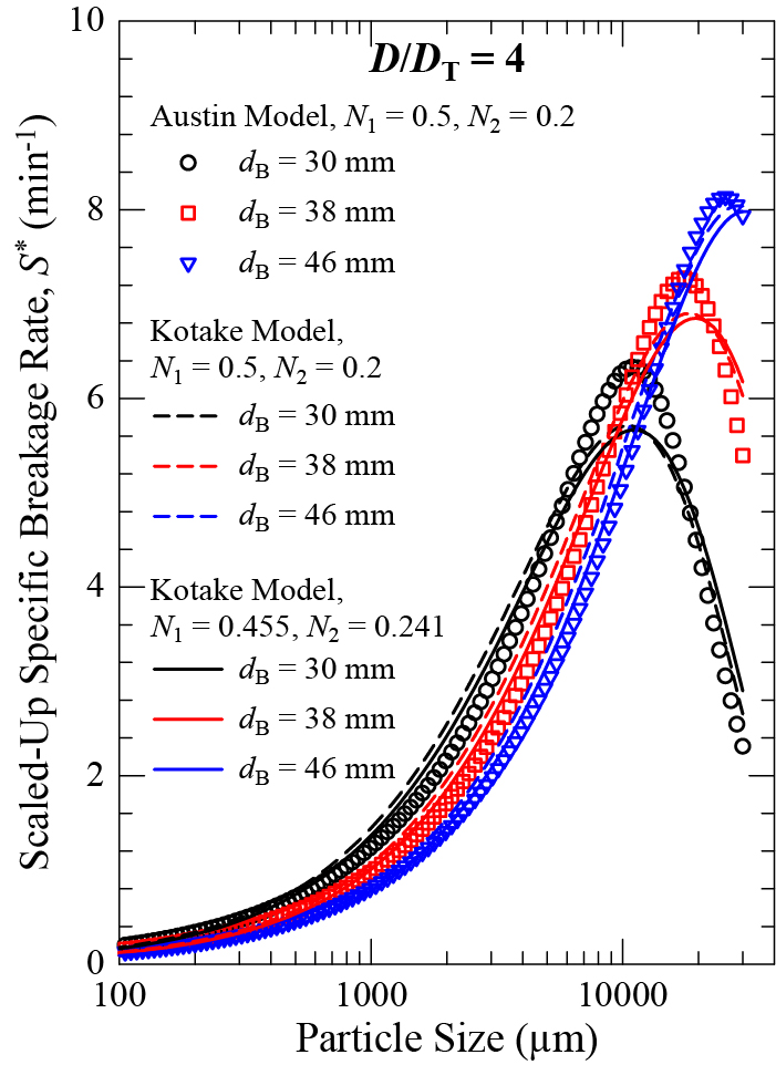
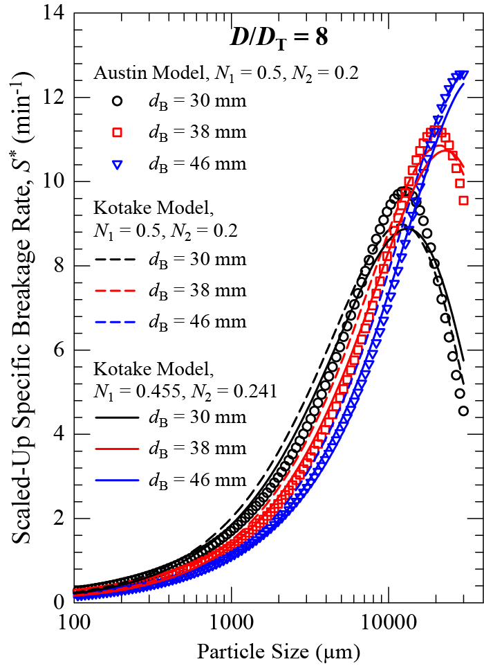
Comparison of S_i^* generated by the Austin model and the KK model with two sets of N₁–N₂ (D/D_T = 8).

A cursory look at Figs. 4 and 5 vs. Fig. 1 reveals the remarkable impact of the scale-up on the specific breakage rate. Upon scale-up and an increase in D/D_T, the specific breakage rate increases, which accords well with the experimental ball milling literature (Austin, 1973; Austin et al., 1984). N₁ captures the increase in mill power as mill diameter increases (Austin, 1973). S_m and x_m also increase, which suggests the maximum point moves to the right and its peak is heightened. With an increase in D/D_T, the cliff after x_i > x_m becomes less pronounced and the abnormal breakage region shrinks. In fact, for d_B = 46 mm, the maximum point almost disappears. Obviously, for a higher D/D_T value, the balls are dropped from a greater height, and they hit the particles at a much higher impact force. According to a semi-theoretical analysis (Hayashi and Tanaka, 1972), the impact force for free-falling balls scales with D^0.5. A recent advanced DEM simulation study (De Carvalho et al., 2021) provides a more fundamental explanation. Their DEM simulations point out a significant expansion of the collision frequency–collision energy envelope as the ball milling is carried out at larger scales: from batch to pilot and then to industrial mills. They determined the specific collision frequency to be 2404 collisions/kg∙s, 2746 collisions/kg∙s, and 3795 collisions/kg∙s at the batch, pilot, and industrial scales, respectively. Overall, higher impact forces, collision energies, and specific collision frequency explain the higher specific breakage rates upon scale-up fundamentally.

The differences in S_i^* between the Austin model and the KK model, with/without the modified N₁ and N₂ exponents, illustrated in Figs. 4 and 5 seem to be unremarkable and most likely statistically insignificant when actual ball milling data are considered. The readers are referred to the discussion and the references in Section 3.1. However, proving this point with comparative experimental study is beyond the scope of this study. We pose a different, yet quite relevant question: can the S_i^* differences depicted in Figs. 4 and 5 translate into significant differences in terms of the PSD evolution with residence time in a continuous mill?

Fig. 6 illustrates that the PSD shifts from the Gaussian feed PSD to the left monotonically along the axial direction of a continuous mill with D/D_T = 4, which is scaled from the small batch mill whose PSD evolution is shown in Fig. 3. The time refers to retention time in the batch mill (Fig. 3) and the residence time in the continuous mill (Fig. 6), which corresponds to different axial locations in the mill. A cursory look at Fig. 6 vs. Fig. 3 reveals that the product becomes much finer upon scale-up, which is in agreement with the higher specific breakage rate parameter upon scale-up (S_i^* in Fig. 4 vs. S_i in Fig. 1). A larger diameter mill with D/D_T = 8 (Fig. 7) exhibits similar behavior; the PSDs are finer as compared with those in Fig. 6, which again can be attributed to the respective S_i^* values in Figs. 4 and 5.

Fig. 6

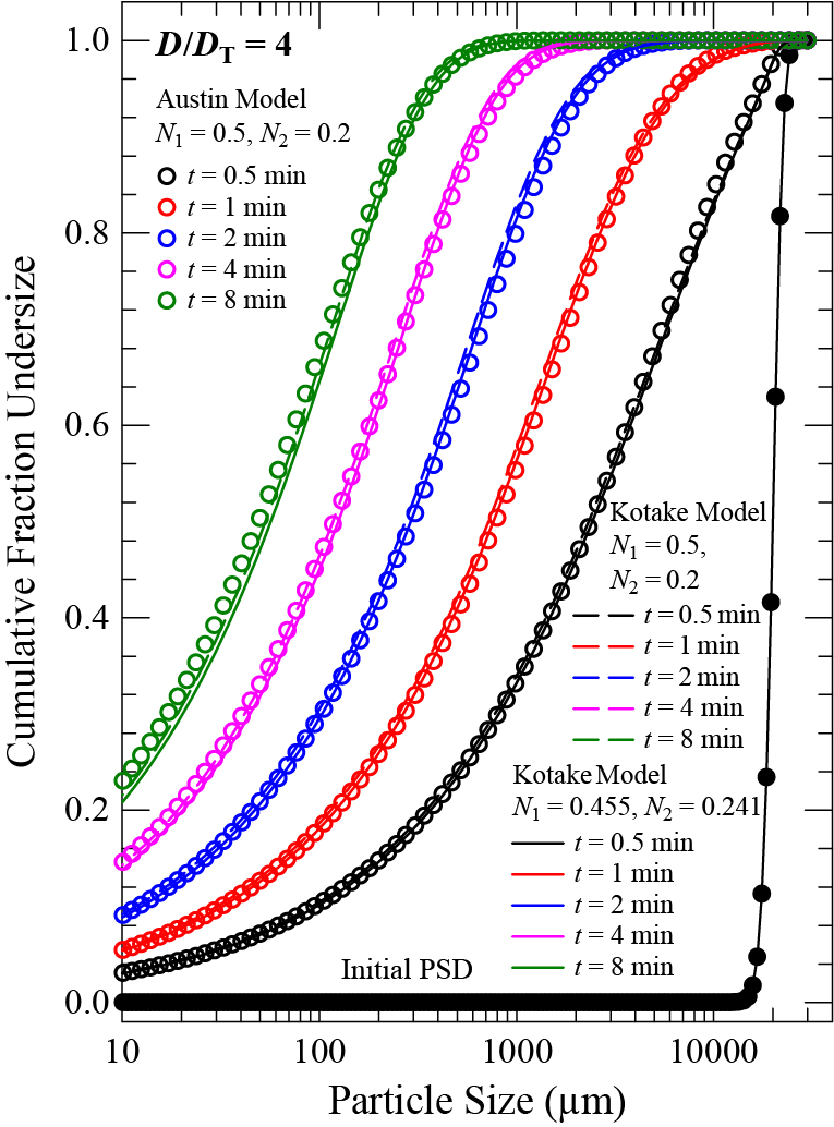
The variation of the PSD at different residence times of the particles (different axial locations) in a continuous ball mill with plug-flow, D/D_T = 4, and d_B = 38 mm.

Fig. 7

The variation of the PSD at different residence times of the particles (different axial locations) in a continuous ball mill with plug-flow, D/D_T = 8, and d_B = 38 mm.

Let us now answer the question posed earlier: the Austin model and the KK model, with either the standard scale-up exponents N₁ = 0.5 and N₂ = 0.2 or the modified scale-up exponents estimated in this study, i.e., N₁ = 0.455 and N₂ = 0.241, predict very similar PSDs in a plug flow continuous mill. Although the differences increased slightly upon scale-up to a larger mill with D/D_T = 8 (Fig. 7), both the Austin model and the KK model estimated similar PSDs, with a max. deviation of 4 % at 10 μm in the cumulative mass fraction.

An interesting finding from the continuous mill simulations presented in Figs. 6 and 7 is that the modification of the Austin’s scale-up exponents N₁ and N₂ was not warranted for the integration of the KK model with the Austin’s scale-up methodology. The KK model with the modified scale-up exponents showed less deviation from the Austin model than that with the standard exponents at the earlier residence time values. However, this trend was reserved at the later residence time points and at the exit of the mill (t = τ = 8 min). Despite the lower SE values of the S_i^* associated with the modified scale-up exponents in Table 2, these differences in the SE values did not seem to make a significant difference in terms of the PSD change along the mill axis and the product PSD, as proven by the simulation results in Figs. 6 and 7. Longer residence times were not considered for two reasons. First, the product PSD (t = 8 min) in the large-scale continuous mills reached the desired target approximately for coal applications: 60– 70 % below 75 μm. Second, the Austin model parameters were estimated using the one-size-fraction data from a ball milling study on South African coal (Katubilwa and Moys, 2009; Katubilwa et al., 2011). In these studies, the smallest feed size fraction studied contained 300–425 μm coal particles. Hence, both the Austin and the KK models extrapolate S_i of the finer particle range (< 300 μm) based on the coarser particles’ breakage kinetics. While this is a common practice, we suspect that the α parameter in both models could be sensitive to the particle size domain in the model calibration. Hence, the slightly higher deviation of the KK model from the Austin model for particles smaller than 100 μm (refer to Fig. 7) could be indirectly linked to the model calibration and the slight differences in the α value (α = 0.81 for the Austin model and α = 0.95 for the KK model).

4. Concluding remarks and outlook

This theoretical study presents a comparative analysis of the Austin kinetic model and the Kotake–Kanda (KK) kinetic model in terms of their prediction of the specific breakage rate parameter as a function of particle size and ball size. Both models have been shown to be similar in terms of their limiting behavior and the extremum behavior because both behaviors are governed by power-law relationships. Mathematical requirements have been formulated to ensure equivalency of both models under these conditions; however, ensuring equivalency for both behaviors through these derived conditions is shown to be severely restrictive or incompatible. Hence, to investigate their similarities further, synthetic specific breakage rate S_i data were generated by the Austin model and fitted by the KK model reasonably well. The PBM simulations of a batch (reference) mill have demonstrated almost identical PSD evolution, confirming the similarity of the two models. Then, a virtual scale-up from the batch reference mill to a continuous plug-flow mill with different D/D_T has been performed. Using the Austin’s scale-up methodology along with the Austin model, the scaled-up specific breakage rate parameter S_i^* has been determined. The KK model has also been scaled-up using the Austin’s scale-up methodology with and without modified scale-up correction exponents. Also, the large-scale continuous mill operation has been simulated via PBM with the S_i^*. This study has overall demonstrated that (i) the KK model is similar, but not equivalent, to the Austin model, (ii) the KK model and the Austin model provide similar PSD evolution after scale-up, (iii) the modification of the Austin’s scale-up exponents N₁ and N₂ is not warranted, and (iv) the Austin’s scale-up methodology is applicable to the KK model as well as the Austin model.

This theoretical study has generated additional questions and ideas for further research. A well-designed experimental ball milling study, using both one-size fraction method and the optimization-based back-calculation method on several natural feed PSDs, should be conducted. The models should be discriminated based on their goodness-of-fit, parameter uncertainties and confidence intervals, and statistical significance. Such studies could reveal if the KK model has some advantages in terms of parameter uncertainties over the Austin model as the former has one less parameter than the Austin model. Such a future study is especially important to the calibration of the KK model (parameter estimation) as the currently used method with one-size-fraction milling experiments is conducive to accumulation of experimental errors. Finally, it is hoped that the Kotake–Kanda model will be used within the Austin’s scale-up methodology for ball mill scale-up in the future.

Acknowledgements

The author would like to thank his PhD student Mr. Nontawat Muanpaopong for preparing the figures and proof-reading the manuscript. This theoretical research did not receive any specific grant from funding agencies in the public, commercial, or not-for-profit sectors.

Data Availability Statement

The data analysis file and the data supporting the findings of this study are available in J-STAGE Data (https://doi.org/10.50931/data.kona.19596367).

References

•  Austin  L.G., Understanding ball mill sizing, Industrial Engineering Chemistry Process Design and Development, 12 (1973) 121–129. DOI:10.1021/i260046a001
•  Austin  L.G.,  Bhatia  V.K., Experimental methods for grinding studies in laboratory ball mills, Powder Technology, 5 (1971–72)261–266. DOI:10.1016/0032-5910(72)80029-9
•  Austin  L.G.,  Luckie  P.T.,  Wightman  D., Steady-state simulation of a cement-milling circuit, International Journal of Mineral Processing, 2 (1975) 127–150. DOI:10.1016/0301-7516(75)90017-4
•  Austin  L.G.,  Shoji  K.,  Luckie  P.T., The effect of ball size on mill performance, Powder Technology, 1 (1976a)71–79. DOI:10.1016/0032-5910(76)80009-5
•  Austin  L.,  Shoji  K.,  Bhatia  V.,  Jindal  V.,  Savage  K.,  Klimpel  R., Some results on the description of size reduction as a rate process in various mills, Industrial & Engineering Chemistry Process Design and Development, 15 (1976b)187–196. DOI:10.1021/i260057a032
•  Austin  L.G.,  Klimpel  R.R.,  Luckie  P.T., Process Engineering of Size Reduction: Ball Milling, Society of Mining Engineers of the AIME, Littleton, CO, USA, 1984, ISBN: 9780895204219.
•  Austin  L.G.,  Julianelli  K.,  De Souza  A.S.,  Schneider  C.L., Simulation of wet ball milling of iron ore at Carajas, Brazil, International Journal of Mineral Processing, 84 (2007) 157–171. DOI:10.1016/j.minpro.2006.09.010
•  Bilgili  E.,  Scarlett  B., Population balance modeling of non-linear effects in milling processes, Powder Technology, 153 (2005) 59–71. DOI:10.1016/j.powtec.2005.02.005
•  Bwalya  M.M.,  Moys  M.H.,  Finnie  G.J.,  Mulenga  F.K., Exploring ball size distribution in coal grinding mills, Powder Technology, 257 (2014) 68–73. DOI:10.1016/j.powtec.2014.02.044
•  Capece  M.,  Bilgili  E.,  Dave  R., Identification of the breakage rate and distribution parameters in a non-linear population balance model for batch milling, Powder Technology, 208 (2011) 195–204. DOI:10.1016/j.powtec.2010.12.019
•  Capece  M.,  Bilgili  E.,  Davé  R., Insight into first-order breakage kinetics using a particle-scale breakage rate constant, Chemical Engineering Science, 117 (2014) 318–330. DOI:10.1016/j.ces.2014.06.019
•  Chimwani  N.,  Glasser  D.,  Hildebrandt  D.,  Metzger  M.J.,  Mulenga  F.K., Determination of the milling parameters of a platinum group minerals ore to optimize product size distribution for flotation purposes, Minerals Engineering, 43–44 (2013) 67–78. DOI:10.1016/j.mineng.2012.09.013
•  Chimwani  N.,  Mulenga  F.K.,  Hildebrandt  D.,  Glasser  D.,  Bwalya  M.M., Scale-up of batch grinding data for simulation of industrial milling of platinum group minerals ore, Minerals Engineering, 63 (2014) 100–109. DOI:10.1016/j.mineng.2014.01.023
•  De Oliveira  A.L.R.,  Tavares  L.M., Modeling and simulation of continuous open circuit dry grinding in a pilot-scale ball mill using Austin’s and Nomura’s models, Powder Technology, 340 (2018) 77–87. DOI:10.1016/j.powtec.2018.09.016
•  De Carvalho  R.M.,  Campos  T.M.,  Faria  P.M.,  Tavares  L.M., Mechanistic modeling and simulation of grinding iron ore pellet feed in pilot and industrial-scale ball mills, Powder Technology, 392 (2021) 489–502. DOI:10.1016/j.powtec.2021.07.030
•  Deniz  V., A study on the specific rate of breakage of cement materials in a laboratory ball mill, Cement and Concrete Research, 33 (2003) 439–445. DOI:10.1016/S0008-8846(02)00976-6
•  Hayashi  M.,  Tanaka  T., Analysis of the selection function of comminution kinetics, Journal of Chemical Engineering of Japan, 5 (1972) 308–310. DOI:10.1252/jcej.5.308
•  Herbst  J.A.,  Fuerstenau  D.W., Scale-up procedure for continuous grinding mill design using population balance models, International Journal of Mineral Processing, 7 (1980) 1–31. DOI:10.1016/0301-7516(80)90034-4
•  Katubilwa  F.M.,  Moys  M.H., Effect of ball size distribution on milling rate, Minerals Engineering, 15 (2009) 1283–1288. DOI:10.1016/j.mineng.2009.07.008
•  Katubilwa  F.M.,  Moys  M.H.,  Glasser  D.,  Hildebrandt  D., An attainable region analysis of the effect of ball size on milling, Powder Technology, 210 (2011) 36–46. DOI:10.1016/j.powtec.2011.02.009
•  King  R.P., Modeling and Simulation of Mineral Processing Systems, Butterworth-Heinemann, Oxford, 2001, ISBN: 0750648848.
•  Klimpel  R.R.,  Austin  L.G., The back-calculation of specific rates of breakage and non-normalized breakage distribution parameters from batch grinding data, International Journal of Mineral Processing, 4 (1977) 7–32. DOI:10.1016/0301-7516(77)90028-X
•  Kotake  N.,  Suzuki  K.,  Asahi  S.,  Kanda  Y., Experimental study on the grinding rate constant of solid materials in a ball mill, Powder Technology, 122 (2002) 101–108. DOI:10.1016/S0032-5910(01)00405-3
•  Kotake  N.,  Daibo  K.,  Yamamoto  T.,  Kanda  Y., Experimental investigation on a grinding rate constant of solid materials by a ball mill—effect of ball diameter and feed size, Powder Technology, 143–144 (2004) 196–203. DOI:10.1016/j.powtec.2004.04.014
•  Kwon  J.,  Cho  H., Investigation of error distribution in the back-calculation of breakage function model parameters via nonlinear programming, Minerals, 11 (2021) 425. DOI:10.3390/min11040425
•  Mulenga  F.K., Sensitivity analysis of Austin’s scale-up model for tumbling ball mills — Part 2. Effects of full-scale milling parameters, Powder Technology, 317 (2017) 6–12. DOI:10.1016/j.powtec.2017.04.043
•  Petrakis  E.,  Stamboliadis  E.,  Komnitsas  K., Identification of optimal mill operating parameters during grinding of quartz with the use of population balance modeling, KONA Powder and Particle Journal, 34 (2017) 213–223. DOI:10.14356/kona.2017007
•  Prasher  C.L., Crushing and Grinding Process Handbook, Wiley, Chichester, 1987, ISBN: 9780471105350.
•  Randolph  A.D.,  Larson  M.A., Theory of Particulate Processes (Second Edition), Academic Press, San Diego, 1988, ISBN: 9780125796521.
•  Rodriguez  V.A.,  De Carvalho  R.M.,  Tavares  L.M., Insights into advanced ball mill modelling through discrete element simulations, Minerals Engineering, 127 (2018) 48–60. DOI:10.1016/j.mineng.2018.07.018
•  Rogers  R.S.C.,  Austin  L.G., Residence time distribution in ball mills, Particulate Science and Technology, 2 (1984) 191–209. DOI:10.1080/02726358408906404
•  Rogers  R.S.C.,  Austin  L.G.,  Brame  K.A, Mill sizing for phosphate grinding in mills of 0.2 to 5 meters in diameter. Mining, Metallurgy & Exploration, 3 (1986) 240–246. DOI:10.1007/BF03402488
•  Sedlatschek  K.,  Bass  L. Contribution to the theory of milling processes, Powder Metallurgy Bulletin, 6 (1953) 148–153.
•  Shahcheraghi  S.H.,  Mulenga  F.K.,  Tavakoli Mohammadi  M.R.,  Mousavi  S.M., How precise are ore breakage parameters measured from direct batch milling tests?, Minerals Engineering, 137 (2019) 157–159. DOI:10.1016/j.mineng.2019.04.010
•  Shampine  L.F.,  Gladwell  I.,  Thompson  S., Solving ODEs with MATLAB, Cambridge University Press, New York, 2003, ISBN: 9780521530941.
•  Tavares  L.M., Chapter 1 Breakage of Single Particles: Quasi-Static, in:  Salman  A.D.,  Ghadiri  M.,  Hounslow  M.J. (Eds.), Handbook of Powder Technology, Elsevier Science B.V., 2007, pp. 3–68, ISBN: 0167-3785. DOI:10.1016/S0167-3785(07)12004-2
•  Tavares  L.M., A review of advanced ball mill modelling, KONA Powder and Particle Journal, 34 (2017) 106–124. DOI:10.14356/kona.2017015
•  Tavares  L.M.,  King  R.P., Single-particle fracture under impact loading, International Journal of Mineral Processing, 54 (1998) 1–28. DOI:10.1016/S0301-7516(98)00005-2
•  Vogel  L.,  Peukert  W., Breakage behaviour of different materials—construction of a mastercurve for the breakage probability, Powder Technology, 129 (2003) 101–110. DOI:10.1016/S0032-5910(02)00217-6
•  Yildirim  K.,  Cho  H.,  Austin  L.G., The modeling of dry grinding of quartz in tumbling media mills, Powder Technology, 105 (1999) 210–221. DOI:10.1016/S0032-5910(99)00140-0

Nomenclature

a_T

model parameter in the Austin model (mm^−α∙min⁻¹)

a₀

value of a_T for specific ball size d_B,0 (mm^−α∙min⁻¹)

b_ij

breakage distribution parameter (−)

B_ij

cumulative breakage distribution parameter (−)

C₁

model parameter in the KK model (mm^−(m+α)∙min⁻¹)

C₂

model parameter in the KK model (mmⁿ⁻¹)

d_B

ball size (mm)

d_B,0

reference ball size (mm)

D

mill diameter (m)

DEM

Discrete Element Modeling

F

inlet mass flow rate (kg∙min⁻¹)

J

ball filling fraction (−)

KK

Kotake–Kanda

K₁–K₅

Austin’s scale-up correction factors (−)

L

mill length (m)

m, n

ball-size exponents in the KK model (−)

M_{B, p}

mass fraction of ball size with index p (−)

M_h

mass hold-up (kg)

M_i

mass fraction in size class i (−)

N

total number of data points (#)

N_C

critical speed (rpm)

N_p

total number of parameters estimated (#)

N_s

total number of size classes, sink size class (#)

N₀–N₄

Austin’s scale-up correction exponents (−)

ODE

Ordinary Differential Equation

P

total number of ball sizes in a ball mixture (#)

PBM

Population Balance Modeling

PSD

Particle Size Distribution

RTD

Residence Time Distribution

SD

standard deviation (mm)

SE

standard error (min^−0.5)

S_i

specific breakage rate parameter (min⁻¹)

S_m

maximum specific breakage rate parameter (min⁻¹)

S_i^*

scaled-up specific breakage rate parameter (min⁻¹)

${\stackrel{\_}{S}}_i$

specific breakage rate parameter for a ball mixture (min⁻¹)

SU

scale-up

t

time (min)

t*

contact or residence time (min)

u

average axial velocity (m∙s⁻¹)

U

void filling fraction (−)

x

particle size (mm)

x_f

feed particle size (mm)

x_m

particle size at which specific rate parameter is maximum (mm)

y

axial position in a continuous mill (m)

α

particle size exponent in both the Austin model and the KK model (−)

β, γ

breakage distribution exponents (−)

ξ, η

constant ball-size exponents in the Austin model (−)

Λ

abnormal breakage exponent in the Austin model (−)

μ_T

a size parameter in the Austin model (mm)

μ₀

value of μ_T for specific ball size d_B,0 (mm)

τ

space-time or average residence time (min)

ϕ

breakage distribution constant (−)

ϕ_C

fraction of operating rotation speed compared to critical speed (−)

i, j

size-class indices

ini

initial

m

maximum

p

ball size index

T

test condition as reference for the scale-up

Author’s Short Biography

Ecevit Bilgili

Dr. Ecevit Bilgili is a Professor, AIChE Fellow, master teacher, and associate chair of the Chemical and Materials Engineering department at NJIT. He holds a PhD in chemical engineering from Illinois Institute of Technology, Chicago, USA. His Particle Engineering and Pharmaceutical Nanotechnology Lab has been conducting research in designing formulations and processes for high-value-added products like pharmaceuticals with enhanced functionalities. His research entails development, optimization, intensification, and scale-up of various particulate processes such as milling, granulation, and drying. Dr. Bilgili also models various milling processes via combined DEM–PBM. He currently serves as the Associate Executive Editor of Advanced Powder Technology journal.