Analysis and Modeling of Non-Spherical Particle Motion in a Gas Flow

Abstract

This paper describes the reviews of the recent works in analysis, modeling, and simulation of the motion of a non-spherical particle. The motion of the non-spherical particles was analyzed in detail by means of a fully resolved direct numerical simulation (DNS). From the DNS data, the PDF-based drag coefficient model was proposed and applied to the particle dispersion simulation in an isotropic turbulent flow to assess the effect of the particle shape by comparing it with the motion of a spherical particle. Moreover, the model was applied to a large-eddy simulation (LES) of particle dispersion in an axial jet flow and validated by comparing it with the experimental data. Results showed that the effect of the particle shape was clearly observed in the characteristics of the particle dispersion in the isotropic turbulent flow by evaluating the deviation from the Poisson distribution (D number) and the radial distribution function (RDF). It was found that the non-spherical particle’s representative Stokes number becomes larger as the sphericity increases. Furthermore, it was also revealed that the effects of the particle size distribution and the shape observed in the experiment was precisely captured by the LES that coincided with the trend found in the isotropic turbulent flow.

1. Introduction

A dispersed gas-particle two-phase flow is frequently utilized in many industrial applications, such as conveyance and energy conversion systems of solid materials. It is an urgent issue to reduce the environmental impact of these facilities for a low-carbon society. To design such highly efficient devices, it is essential to deeply understand the behavior of particles in a fluid flow.

A non-spherical particle is frequently seen in the industry as a pulverized solid particle such as coal which may behave in a different motion from a spherical particle. A great many efforts have been conventionally made to investigate the motion of the non-spherical particle. The majority of the works were dedicated to a spheroidal particle. Feng J. et al. (1995) performed a three-dimensional computation of the force and torque acting on an ellipsoid settling slowly in a viscoelastic fluid. They found that the signs of the perturbation pressure and velocity around the particle for inertia were reversed by viscoelasticity and the torques were also opposite signs. It was also found that the equilibrium tilt angle was a function of the elasticity number which was the ratio of the Weissenberg number and the Reynolds number. Broday D. et al. (1998) investigated the motion of non-neutrally buoyant prolate spheroidal particles freely rotating or fixed with orientations in vertical shear flows. They revealed that the spheroids freely moving translated along periodic trajectories with no net lateral drift, whereas the particles with fixed orientations were unstable with the drift velocity growing exponentially with time. The conditions for the unstable motion were also discussed as a function of the particle shape, via its aspect ratio and its inertia. Mortensen P.H. et al. (2008) performed a direct numerical simulation (DNS) of prolate ellipsoidal particles suspended in a turbulent channel flow. It was found that the ellipsoidal particles tend to align with the mean flow direction in the near-wall region, while the orientation became isotropic in the core region. In addition, when the particle inertia increases, the particles were less oriented in the spanwise direction and more oriented in the wall-normal direction.

Mathematical modeling of the complex motion of the non-spherical particle has been also examined in many works. Haider A. and Levenspiel O. (1989) proposed the explicit equations for the drag coefficient of falling non-spherical particles by fitting the experimental data of isometric and disk type solids with classification in terms of the sphericity. In this work, the drag coefficient is a function of the sphericity and Reynolds number, and the orientation is not considered. Holzer A. and Sommerfeld M. (2008) also proposed a simple correlation formula for the drag coefficient of arbitrarily shaped particles by introducing the crosswise and lengthwise sphericities in addition to the normal sphericity into the drag coefficient equation based on a number of the experimental and numerical studies. Rosendahl L. (2000) developed the particle shape description based on the minor axis, the aspect ratio, and the superelliptic exponent to account for the shape effect of ellipsoids and cylinders and Zastawny M. et al. (2012) extended the model to account for the drag force, the lift force, the pitching torque, and the torque caused by the rotation of the particles based on the fully resolved DNS. They should be in useful forms when the orientation of the particle is considered in a Lagrangian particle tracking simulation.

In the modeling of the motion of the non-spherical particle in the earlier stage, the sphericity is simply used to consider the effect of the non-sphericity on the drag coefficient and the other related parameters to characterize the particle motion, while it cannot consider the effect of oscillation and rotating in a fluid flow. In the later stage, the effect of rotation is considered by introducing the orientation such as the crosswise and lengthwise sphericities. In the CFD framework, conventionally the Reynolds-averaged Navier-Stokes (RANS) simulation in which the entire scale of the turbulent eddy is modeled and the time-averaged quantities are evaluated is mainly used as a standard tool to predict the particle behavior in the industry due to its lower computational cost in spite of its lower accuracy for a long time (e.g Watanabe H. and Otaka M. (2006), Watanabe H. et al. (2015), Hashimoto N. and Watanabe H. (2016)). However, with the great advance in computer performance, massively parallel large-scale computing by means of a large-eddy simulation (LES) in which the eddies in the subgrid-scale are only modeled and the fully unsteady phenomena can be considered is expected to be a new standard tool (e.g. Kurose R. et al. (2009), Muto M. et al. (2019), Ahn S. et al. (2019), Watanabe H. and Kurose R. (2020)). In such a highly fidelity unsteady simulation framework, the motion models which can consider the oscillation and rotation of the particle would be essential.

While the models taking the orientation of the particles into account have been proposed in some existing works, as mentioned earlier, another modeling strategy will be reported hereafter in this paper. In typical industrial applications, a tremendous number of particles exist in a fluid flow such as a pulverized coal combustion boiler. Here we introduce a concept of probability density function (PDF) to model the motion of non-spherical particles. In Section 2, the motion model of the non-spherical particle is developed by a fully resolved DNS. In Section 3, the model proposed here is assessed in an isotropic turbulent flow by means of a DNS with the point mass approximation. In Section 4, the model is applied to an LES of a turbulent axial jet flow and validated with the experiment.

2. Modeling of non-spherical particle motion

In this section, the motion of a single non-spherical particle is numerically investigated by means of a fully resolved gas-particle two-phase flow DNS. The DNS data is analyzed to formulate the effects of the non-sphericity in the motion equation. The Basset-Boussinesq-Oseen (B.B.O.) equation is expressed as,

  

$${\rho }_{\text{p}}{V}_{\text{p}}\frac{\text{d}\mathit{v}}{\text{d}t}={\mathit{F}}_{\text{D}}+{\mathit{F}}_{\text{L}}+{\mathit{F}}_{\text{B}}+{\mathit{F}}_{\text{prs}}+{\mathit{F}}_{\text{mass}}+{\mathit{F}}_{\text{Basset}},$$(1)

where ρ_p, V_p, and v are the density, volume, and velocity of the particle, respectively. F_D, F_L, F_B, F_prs, F_mass, and F_Basset are the drag force, lift force, buoyancy, pressure gradient, virtual mass, and Basset history term, respectively. In this study, because the drag force mainly contributes to the motion of the particle in the pulverized coal combustion field, we pay special attention to F_D via modeling of the drag coefficient C_D.

The drag force is regarded as the summation of the contributions of the pressure and frictions as,

  

$${\mathit{F}}_{\text{D}}={\mathit{F}}_{\text{Dprs}}+{\mathit{F}}_{\text{Dfrc}}.$$(2)

And the drag coefficient can be also expressed as,

  

$$C_{\text{D}}=\frac{{\mathit{F}}_{\text{D}}}{\frac{1}{2}{\rho }_{\text{f}}{|\mathit{u}-\mathit{v}|}^{2}A}=C_{\text{Dprs}}+C_{\text{Dfrc}},$$(3)

where A is the projection area of the particle to the flow direction. As shown in Eqn. (3), C_D is also considered as a sum of C_Dprs and C_Dfrc which are influenced by the pressure and the friction, respectively. C_D for a spherical particle can be regarded as a simple function of the Reynolds number Re and as mentioned earlier, many works propose the drag curve equations. Clift R. et al. (1978) summarized some of the most popular expressions, and provided the following recommendation as,

  

$$C_{\text{D}}=3/16+24/Re\mathrm{\hspace{0.17em} }\mathrm{\hspace{0.17em} }\mathrm{\hspace{0.17em} }\text{for\hspace{0.28em}}\mathrm{\hspace{0.17em} }\mathrm{\hspace{0.17em} }\mathit{\text{Re}}<0.01,$$(4)

  

$$C_{\text{D}}=\frac{24}{Re}(1+0.1315R{e}^{0.82-0.05·\text{log}\hspace{0.17em}Re})\mathrm{\hspace{0.17em} }\mathrm{\hspace{0.17em} }\mathrm{\hspace{0.17em} }\text{for\hspace{0.28em}}\mathrm{\hspace{0.17em} }\mathrm{\hspace{0.17em} }0.01<Re\le 20,$$(5)

  

$$C_{\text{D}}=\frac{24}{Re}(1+0.1935R{e}^{0.6305})\mathrm{\hspace{0.17em} }\mathrm{\hspace{0.17em} }\mathrm{\hspace{0.17em} }\text{for\hspace{0.28em}}\mathrm{\hspace{0.17em} }\mathrm{\hspace{0.17em} }20<Re\le 260,$$(6)

where Re is based on the slip velocity and particle size as,

  

$$Re=\frac{{\rho }_{\text{f}}|\mathit{u}-\mathit{v}|d}{\mu },$$(7)

where d is the diameter of the particle and μ is the viscosity of the fluid, respectively.

Eqns (1) to (6) are only suitable for a spherical particle. A non-spherical particle is typically assessed by the sphericity which is defined as the ratio of the surface area of a sphere to that of a given particle where the sphere and the given particle have the same volume as,

  

$$\varphi =\frac{S_{\text{sphere}}}{S_{\text{particle}}}=\frac{{\pi }^{1/3}{(6V_{\text{particle}})}^{2/3}}{S_{\text{particle}}}.$$(8)

According to the examination by Haider A. and Levenspiel O. (1989), C_D becomes larger as ϕ decreases.

2.1 The arbitrary Lagrangian-Eulerian (ALE) method

To deeply understand the six-degree of freedom for a particle motion, the arbitrary Lagrangian-Eulerian (ALE) method is employed (Hirt C.W. et al. (1974)). The governing equations of the ALE method are expressed as,

  

$$\frac{\partial {\rho }_{\text{f}}}{\partial t}+((\mathit{u}-{\mathit{u}}^{\prime })·\nabla )\hspace{0.17em}{\rho }_{\text{f}}=-{\rho }_{\text{f}}\nabla ·\mathit{u},$$(9)

  

$$\frac{\partial \mathit{u}}{\partial t}+((\mathit{u}-{\mathit{u}}^{\prime })·\nabla )\hspace{0.17em}\mathit{u}=-\frac{1}{{\rho }_{\text{f}}}\nabla p+\frac{1}{{\rho }_{\text{f}}}\nabla p·\mathit{\sigma }+\mathit{g},$$(10)

where ρ_f and u are the fluid density and velocity, respectively, u′ the mesh velocity, p the pressure, σ the surface stress tensor. The ALE method is equivalent to the Eulerian method when u′ = 0 and is equivalent to the Lagrangian method when u′ = u. Here, the particle velocity v is employed as u′ to consider the Lagrangian particle motion. The slip velocity u – v appears when the particle translates, rotates and oscillates. This means that the entire computational grid around the particle moves in the ALE method.

The motion of the single particle is calculated by the governing equations of a rigid body as,

  

$$m\frac{{\text{d}}^2\mathit{z}}{\text{d}{t}^2}=\mathit{F},$$(11)

  

$$\mathit{I}\frac{{\text{d}}^2\mathit{\alpha }}{\text{d}{t}^2}+\frac{\text{d}\mathit{\alpha }}{\text{d}t}\times \left(\mathit{I}\frac{\text{d}\mathit{\alpha }}{\text{d}t}\right)=\mathit{M},$$(12)

where m is the particle mass, I the moment of inertia of particle, z the displacement angle, α the rotation angle, F the force on the particle, M the torque on the particle, which are obtained by considering the integration of the fluid force over the surface and the gravity. Subsequently, we can calculate the moving and angular velocities of the particle. The presented numerical procedure was implemented into the unstructured FVM parallel computing solver FFR-Comb (NuFD/FrontFlowRed extended by Kyushu Univ., Kyoto Univ., CRIEPI, and NuFD) (Zhang W. et al., 2018a; 2018b). The presented ALE method has been properly validated by comparing with the correlation expression of the drag coefficient curve by Clift R. et al. (1978) and with the experiment of the falling particles in water by Mordant N. et al. (2000). See more details of this DNS in Zhang W. et al. (2018b).

2.2 Computational details

To observe the motion characteristics of various particle shapes, pulverized coal and spheroidal particles are examined. Fig. 1 shows the shapes of the particles. The 3D data of the coal particle was obtained by the X-ray CT scanner. The shape of the spheroidal particle was determined by the equivalent volume. In our preliminary examination, the spheroid with the equivalent volume shows the closest behavior of the coal particle rather than the spheroids with the equivalent surface area and sphericity. Fig. 2 shows the computational grid for the coal particle. The computational domain is discretized with about 12 million cells and is divided into 1,024 regions for the MPI parallel computing. It takes approximately 15,000 node-hour for one case. The grid resolution around the particle is confirmed to be enough to resolve the boundary layer thickness formed on the surface within the range of the particle Reynolds number Re in this study following the theorem by Schlichting et al. (1955) and the examination by Muto et al. (2012).

Fig. 1

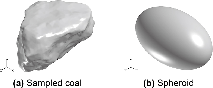
Shapes of (a) sampled pulverized coal particle, and (b) spheroid with equivalent volume. Reprinted with permission from Ref. (Zhang et al., 2018a). Copyright: (2018) Elsevier B.V.

Fig. 2

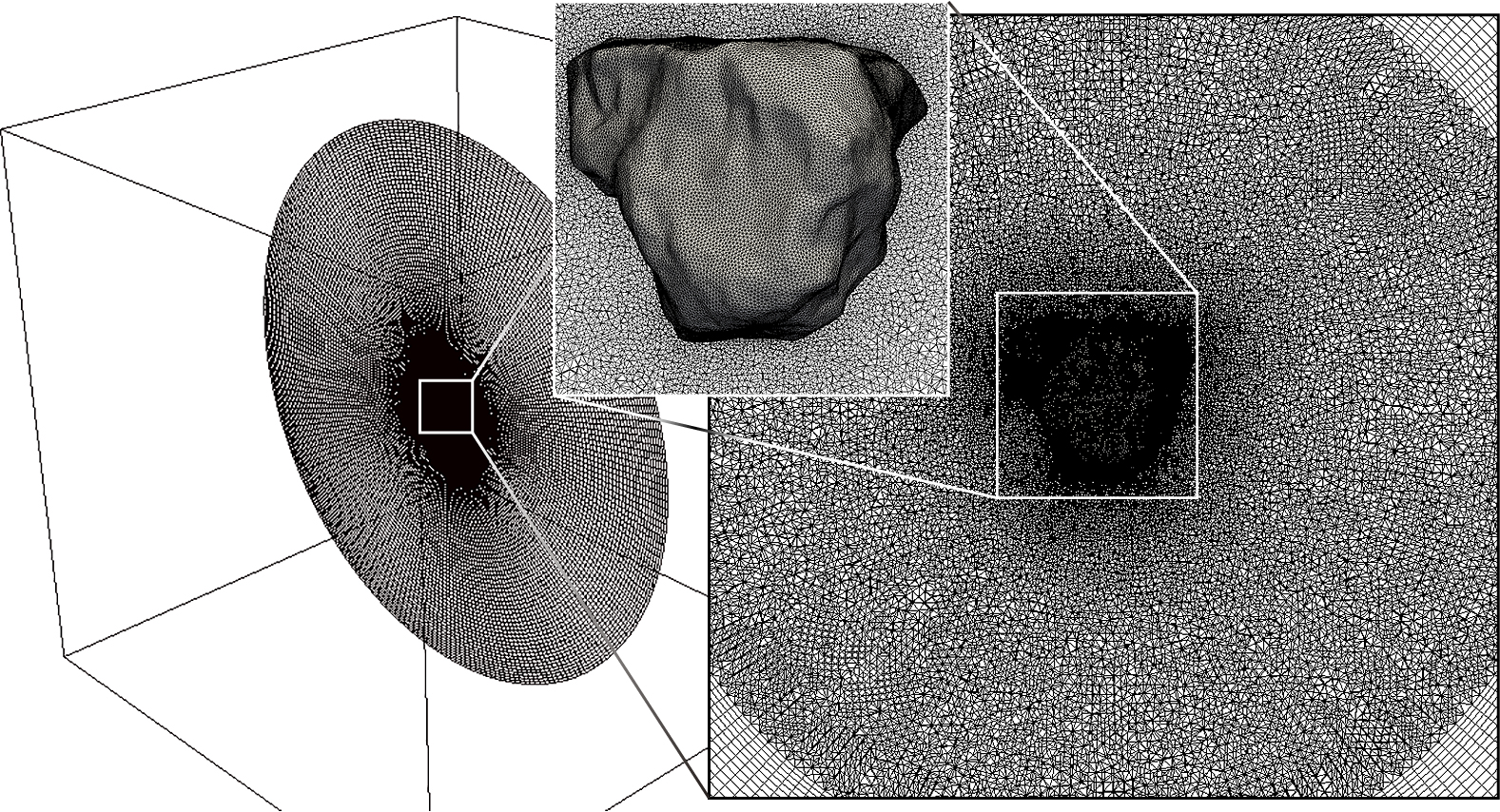
Computational grid for sampled coal particle. Reprinted with permission from Ref. (Zhang et al., 2018a). Copyright: (2018) Elsevier B.V.

The flow velocity was set to 15 m/s, and the particle was placed in the upward flow at the beginning of the computation. The particle was released at t = 0 without the initial velocity. The major axis of each particle was set in the vertical direction. The initial Re was estimated as 45.

2.3 Results and discussion

Fig. 3 shows the drag curves for (a) coal particle and (b) spheroid with the equivalent volume. In Fig. 3, C_Dprs and C_Dfrc are also displayed as well as C_D. It is found that the C_D curve oscillates for the both particles. Because the major axis is set in the vertical direction, the initial projection area in the fluid direction is small and it is located in unstable equilibrium. With the small disturbance of the pressure or friction variation on the surface, the particle starts oscillating and rotating. It is found that the contribution of C_Dfrc is dominant, while the large oscillation is observed for C_Dprs. It is also understood that the trend for the spheroid shows a good agreement with that for the coal particle.

Fig. 3

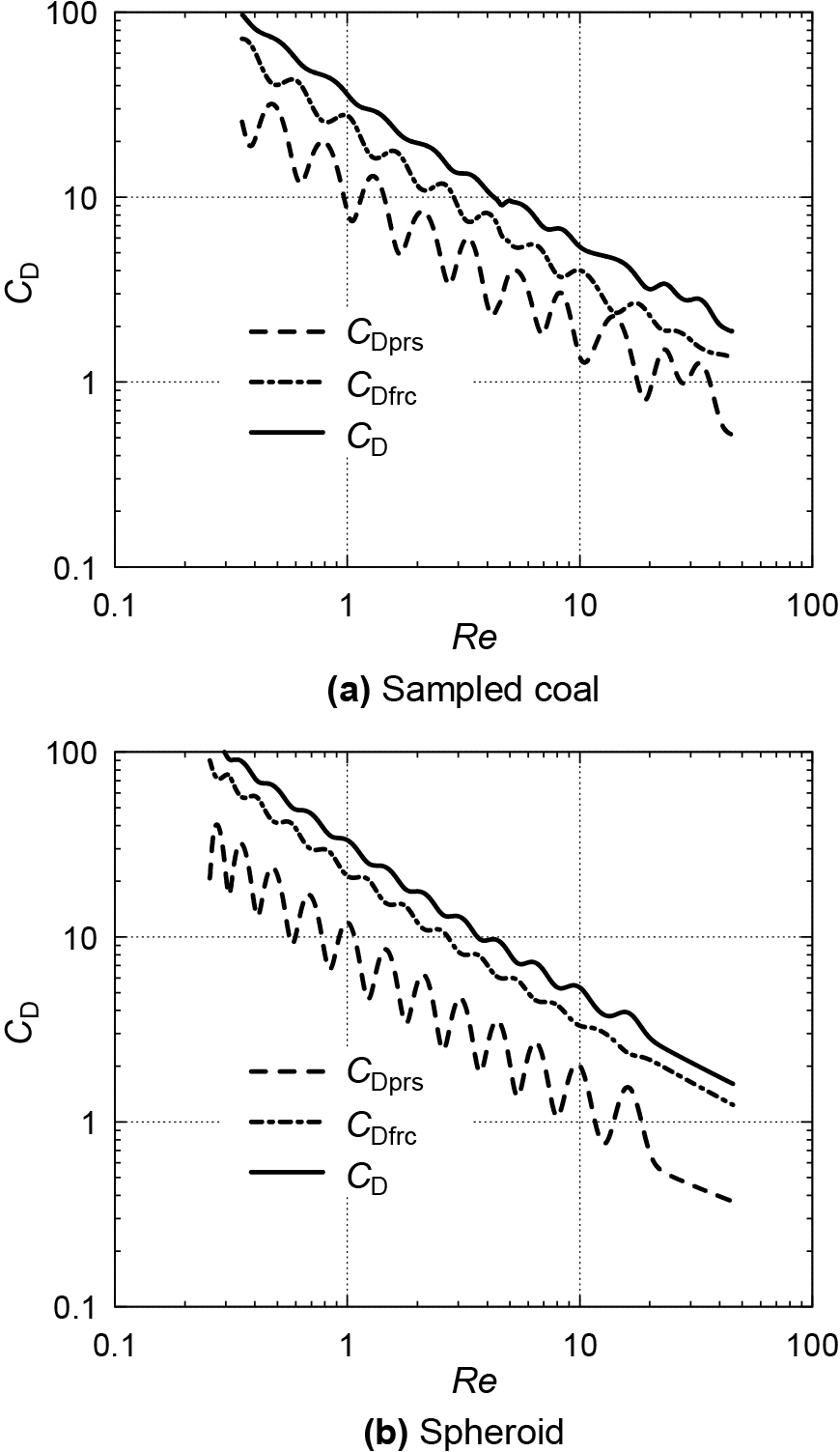
Drag curves for (a) sampled pulverized coal particle, and (b) spheroid with equivalent volume. Reprinted with permission from Ref. (Zhang et al., 2018a). Copyright: (2018) Elsevier B.V.

Fig. 4 shows the drag curves with the various initial angles of the major axis of the spheroid. Here, the two-digit number after “EV” (equivalent to the volume) in the figure displays the initial angle from the horizontal axis. In spite of the difference in the timing to start the oscillation among the cases, all the oscillating curves are located within a certain range of the maximum and minimum smooth curves. The trend of the oscillation is analyzed in terms of the probability density in Fig. 5. Here, the probability density function (PDF) of the sine curve is displayed as well in Fig. 5. It is revealed that the PDF of the sine curve can precisely reproduce that of the spheroid particle. From this consideration, the characteristics of the oscillating C_D can be formulated by the following simple expression as,

  

$$\text{log}{C}_{\text{D}}=\text{log}{C}_{{\text{D}}_{\text{min}}}+\left(\text{log}{C}_{{\text{D}}_{\text{max}}}-\text{log}{C}_{{\text{D}}_{\text{min}}}\right)·\frac{\text{sin\hspace{0.17em}}(2\pi \theta +1)}{2},$$(13)

where θ is the random number from 0 to 1, and C_Dmax and C_Dmin are determined by the computation of the six-degree of freedom motion of the target particle and those can be approximated by the expressions by Haider A. and Levenspiel O. (1989) and Clift R. et al. (1978) as,

  

$$C_{\text{D}}=\frac{24}{Re}(1+A\hspace{0.17em}R{e}^{B-C·\text{log\hspace{0.17em}}Re})\mathrm{\hspace{0.17em} }\mathrm{\hspace{0.17em} }\mathrm{\hspace{0.17em} }\text{for\hspace{0.28em}}\mathrm{\hspace{0.17em} }\mathrm{\hspace{0.17em} }0.01<Re\le 10,$$(14)

  

$$C_{\text{D}}=\frac{24}{Re}(1+X\hspace{0.17em}R{e}^{\text{Y}})\mathrm{\hspace{0.17em} }\mathrm{\hspace{0.17em} }\mathrm{\hspace{0.17em} }\text{for\hspace{0.28em}}\mathrm{\hspace{0.17em} }\mathrm{\hspace{0.17em} }10<Re\le 100.$$(15)

Here, the model parameters, A, B, C, X, and Y are determined by the computation as mentioned earlier.

Fig. 4

Drag curves for spheroid with equivalent volume with various initial angles. Reprinted with permission from Ref. (Zhang et al., 2018a). Copyright: (2018) Elsevier B.V.

Fig. 5

PDFs of drag coefficient for spheroid and sine curve. Reprinted with permission from Ref. (Zhang et al., 2018a). Copyright: (2018) Elsevier B.V.

3. Dispersion of non-spherical particles in an isotropic turbulent flow

In this section, the non-spherical particle motion model developed in the previous section is applied to the Eulerian-Lagrangian two-way coupling DNS with employing the particle-source-in cell (PSI-CELL) model (Crowe C.T. et al. (1977)) to observe the effects of non-sphericity.

3.1 Governing equations

The governing equations for the fluid flow consist of the mass and momentum conservations as,

  

$$\frac{\partial {\rho }_{\text{f}}}{\partial t}+\frac{\partial {\rho }_{\text{f}}{u}_j}{\partial x_j}=0,$$(16)

  

$$\frac{\partial {\rho }_{\text{f}}{u}_i}{\partial t}+\frac{\partial {\rho }_{\text{f}}{u}_j{u}_i}{\partial x_j}=-\frac{\partial p}{\partial x_i}+\frac{\partial {\sigma }_{ij}}{\partial x_j}+S_{u_i},$$(17)

where u_i and σ_ij are the fluid velocity and stress tensor, respectively. S_ui is the source term of the interphase momentum transfer and evaluated by,

  

$$S_{u_{\text{i}}}=-\frac{1}{\mathrm{\Delta }V}{\sum }_{}^N\frac{m}{{\tau }_{\text{p}}}\frac{Re}{24}{C}_{\text{D}}(u_{\text{i}}-u_{\text{p}}),$$(18)

where u_p is the particle velocity and ΔV the control volume. τ_p is the particle response time. The stokes number St charactering the behavior of particles in a fluid flow is defined with the Kolmogorov time scale τ_k as,

  

$$St=\frac{{\tau }_{\text{p}}}{{\tau }_{\text{k}}}.$$(19)

The particles are treated as mass points and tracked by the Lagrangian manner. The gravity and lift forces are ignored. The effects of the pressure gradient, virtual mass, and Basset history term are neglected. The motion equations for the particles are expressed as,

  

$$\frac{\text{d}{x}_{\text{p}}}{\text{d}t}=u_{\text{p}},$$(20)

  

$$\frac{\text{d}{u}_{\text{p}}}{\text{d}t}=\frac{1}{{\tau }_{\text{p}}}\frac{Re}{24}{C}_{\text{D}}(u_{\text{i}}-u_{\text{p}}),$$(21)

where x_p is the particle position.

3.2 Computational details

Fig. 6 shows the computational domain displaying the distribution of the vortices distinguished by the second invariant of the velocity gradient tensor, Q = 10,000. The domain is a (2π)³ cm³ cube divided by 128³ grids. All boundaries are set as periodic boundaries. The isotropic turbulent field generated in this study has the RMS (root mean square) of the velocity of 2.7 m/s and the Taylor’s microscale-based Reynolds number of 60 which is closed to the condition by Ooi A. et al., (1999). The isotropic turbulent flow is evaluated by the energy spectrum field and St is controlled by varying the particle size. The one spherical and five different sphericity spheroidal particles are examined. Table 1 shows the particle properties. All the model parameters for each particle shape are obtained by the computation of the six-degree of freedom motion of the target particle as described in Section 2. See more details of this DNS in Zhang W. et al. (2018b).

Fig. 6

Computational domain and vortex visualization of isotropic turbulent flow. Reprinted with permission from Ref. (Zhang et al., 2018a). Copyright: (2018) Elsevier B.V.

Table 1

Cases performed in isotropic turbulent flow.

Cases	Sphericity [−]	Diameter of equivalent volume sphere [m]
SV	1.00	4.23 × 10−5
EL96	0.96	4.23 × 10−5
EL90	0.90	4.23 × 10−5
ES90	0.90	3.43 × 10−5
EL85	0.85	4.23 × 10−5
ES85	0.85	2.91 × 10−5

3.3 Results and discussion

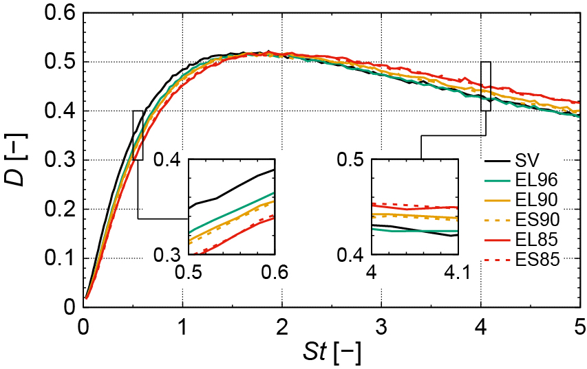
The characteristics of the particle dispersion is evaluated by the D number (Fessler J.R. et al. (1994)) which shows the deviation between the target particles dispersion and the Poisson distribution defined as,

  

$$D=\frac{\sigma -{\sigma }_{\text{Poi}}}{\lambda },$$(22)

where σ and σ_Poi are the standard deviations, and λ is the mean number of particles in each small box which is set to analyze D. In this study, 24³ boxes are applied to the whole domain. Fig. 7 shows the variation of D with the various St for the six cases. It is found that the effect of the sphericity changes at the point where the peak value of D appears. In the region of the smaller St from the point of the peak, D becomes larger with increasing the sphericity. On the other hand, in the larger St region, the trend is opposite. In other words, as the sphericity increases, the D curve shifts toward the larger St direction. This means that the spheroid’s apparent (representative) Stokes number St′, which represents the dispersion behavior becomes larger.

Fig. 7

Computational domain and vortex visualization of isotropic turbulent flow. Reprinted with permission from Ref. (Zhang et al., 2018a). Copyright: (2018) Elsevier B.V.

The characteristics of the particle dispersion is also analyzed by the radial distribution function (RDF) which describes the characteristics of particle clustering in terms of its length scale. RDF is defined as,

  

$$g\left(r_i\right)=\frac{N_{\text{p}}(i)/\mathrm{\Delta }{V}_i}{N_{\text{p}}/V},$$(23)

where N_p = N(N – 1)/2 is the total number of particle pairs and V is the volume of the whole domain. N_p(i) is the total number of particle pairs with a distance between r_i + Δr/2 and r_i – Δr/2. ΔV_i is the volume of the shell located at a distance r_i with the thickness Δr. Fig. 8 shows the RDF variation with varying St for the representative four cases. In Fig. 8, RDF is evaluated as the sum of g(r) conditioned by r/η < 12, where η is the Kolmogorov length scale. In the condition to analyze D, r/η can be approximately estimated as around 12. It is found in Fig. 8 that as St increases, g(r) initially increases and then decreases after appearing the peak value at St = 1.0 except SV. These trends agree with the result observed in Fig. 7.

Fig. 8

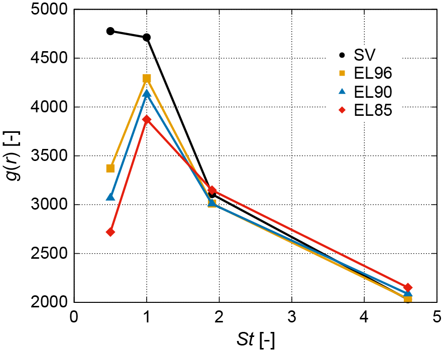
Sum of g(r) values conditioned by r/η < 12 for each case. Reprinted with permission from Ref. (Zhang et al., 2018a). Copyright: (2018) Elsevier B.V.

4. Dispersion of non-spherical particles in a turbulent jet flow

In this section, the non-spherical particle motion model developed in Section 2 is applied to the Eulerian-Lagrangian two-way coupling LES to investigate the particle dispersion behavior in a more practical condition. The model results are compared with the experimental results.

4.1 Governing equations

The governing equations of the fluid and particle motions are almost the same as described in Section 3, while the variables are evaluated with the spatial and Favre filtering in the coarser grid. The subgrid-scale (SGS) terms are considered by the dynamic Smagorinsky model proposed by Moin P. et al. (1991). The interphase momentum transfer is evaluated by the PSI-CELL method.

4.2 Experimental and computational details

Fig. 9 shows the schematic diagram of the targeted cold flow experiment. The particles are transported by the airflow and injected vertically by the coaxial jet burner. The particle image velocimetry (PIV) method is used to measure particle motion. The laser sheet is applied at different heights of 0, 20, 30, 60, 90, 120, 150, 180, and 210 mm from the burner exit. At each height, 1,000 graphics are taken and processed to obtain the time-averaged profiles. In the experiment, the two cases, pulverized coal, and spherical polymer particles are used to observe the effect of the particle’s shape. The densities of coal and polymer are almost the same about 1,200 kg/m³. The averaged flow velocity is set to 7.59 m/s and the particle mass flux is set to 1.29 × 10⁻⁴ kg/s. Fig. 10 shows the particle mass flux of the different diameters.

Fig. 9

Schematics of experimental configuration. Reprinted with permission from Ref. (Zhang et al., 2018b). Copyright: (2018) Elsevier B.V.

Fig. 10

Particle mass fluxes of different diameters for monodispersed and polydispersed cases.

The computational domain is a 360 mm height cylinder with a diameter of 100 mm. The axial jet burner is located at the center of the bottom which has a 6 mm diameter and 60 mm height. The number of cells is 11.5 million. Table 2 shows the four cases performed in this study. As shown in Fig. 10, the particle size distribution is expressed by the representative six diameters in the simulation. The model parameters in Eqns. (14) and (15) for the spheroidal particle with the sphericity of 0.85 are employed to approximate the non-spherical coal particle behavior.

Table 2

Cases performed in turbulent axial jet flow.

Cases	Particle shape (model)	Diameter [m]	Note
COAL	Non-spherical	Polydispersed	Exp
POLYMER	Spherical	2.8 × 10−5	Exp
SPE_S	Spherical	2.8 × 10−5	CFD
SPE_R	Spherical	Polydispersed	CFD
SPO_S	Spheroid	2.8 × 10−5	CFD
SPO_R	Spheroid	Polydispersed	CFD

4.3 Results and discussion

Fig. 11 shows the instantaneous and the time-averaged distributions of the Mie scattering intensity obtained by the experiment for (a) pulverized coal COAL and (b) monodispersed polymer POLYMER, and the distributions of the particle number density by the simulation for (c) monodispersed sphere SPE_S, (d) polydispersed sphere SPE_R, (e) monodispersed spheroid SPO_S, and (f) polydispersed spheroid SPO_R, respectively. Here, the left-hand side of each figure displays the instantaneous distribution, and the right-hand side displays the time-averaged distribution. With focusing on the experimental result, the region that shows the high intensity of Mie scattering for COAL appears near the burner nozzle exit, while that for POLYMER appears at the downstream region from the nozzle exit. For POLYMER the number density of the particles increases once due to the interaction between the turbulent eddies and the particles, while the particles for COAL simply disperse the downstream. In the higher region, the difference turns clearer. POLYMER clusters strongly from the middle to the higher region. In the simulation result, the same concentration downstream from the nozzle exit can be found for the monodispersed cases, SPE_S and SPO_S, while the simple dispersion is observed for the polydispersed cases, SPE_R and SPO_R. The trend obtained by the simulation agrees with that observed in the experiment. It can be considered that the difference in the region where the peak value of the Mie scattering intensity appears between the two cases in the experiment is mainly attributed to the particle size distribution. It is also found that the higher number density region appears downstream for the spheroid cases rather than that for the sphere cases. This is affected by the difference in the particle shape. In the higher region, while the polydispersed cases tend to randomly disperse in space, the monodispersed cases cluster and form the branch-shaped structure.

Fig. 11

Mie scattering intensity in experiments (a) COAL and (b) POLYMER, and number density in CFD (c) SPE_S, (d) SPE_R, (e) SPO_S, and (f) SPO_R. Reprinted with permission from Ref. (Zhang et al., 2018b). Copyright: (2018) Elsevier B.V.

Fig. 12 shows the instantaneous distribution of the particles near the burner nozzle exit for the sphere cases, (a) SPE_S and (b) SPE_R. For SPE_R, the number of the smaller particles which have a short response time is large. They are entrained well by the vortices and the ring-like structure is formed at the nozzle exit. For SPE_S, since the particles are larger enough to be less likely to trace the vortices due to the longer response time than those observed in SPE_R, the ring-like structure does not appear.

Fig. 12

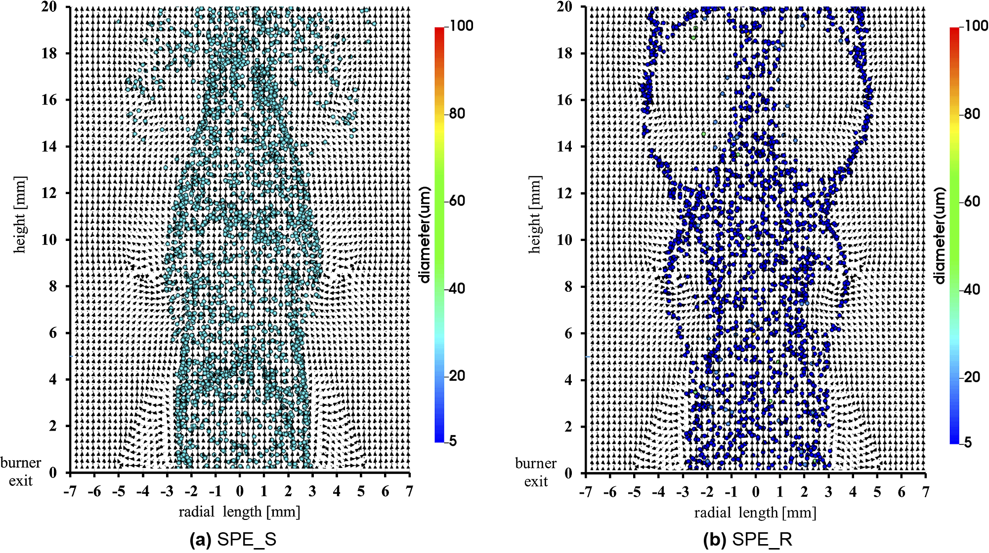
Instantaneous particle distribution near burner nozzle exit for (a) SPE_S and (b) SPE_R. Reprinted with permission from Ref. (Zhang et al., 2018b). Copyright: (2018) Elsevier B.V.

Fig. 13 shows the time-averaged width of the region where the traveling particles exist (the dispersion width) in the axial direction. The particle dispersion width monotonously increases in the axial direction for all cases. Between the sphere cases, since the dispersion width for SPE_R is larger than that for SPE_S in the entire region, the particle size distribution significantly affects the dispersion width. On the other hand, between the spheroid cases, the difference in the dispersion width is not observed. It is considered that the particle shape affects the dispersion width.

Fig. 13

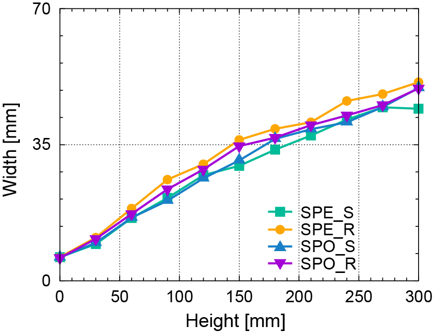
Variation of particle dispersion width in axial direction.

The characteristic length of the particle clustering is analyzed by RDF as described in the previous section. Fig. 14 shows the variation of RDF in the characteristic length scale. It is found that RDF is significantly affected by the particle size distribution, since the monodispersed cases and the polydispersed cases respectively show the individual trend. While RDFs for SPE_S and SPO_S are almost the same in the upstream region at z = 30 mm, SPE_R shows a higher value than SPO_R in the shorter length scale region. In the middle stream at z = 90 mm, the difference between SPE_R and SPO_R becomes smaller, whereas the value for SPO_S becomes slightly higher than that for SPE_S. And then, in the downstream region at z = 180 mm, RDF for SPE_R almost agrees with that for SPO_R, while the difference between SPE_S and SPO_S becomes marked. From this observation, it is revealed that the effect of the particle shape on their dispersion becomes marked toward the downstream, although the particle size distribution tends to suppress this trend. This behavior should be characterized by the Stokes number. The non-sphericity of the particle changes its apparent Stokes number. In the region where the apparent Stokes number is smaller than the order of unity, the particle dispersion is suppressed, and in contrast, the particle dispersion is enhanced by the larger apparent Stokes number, as discussed in the previous section. It is considered that the trend observed in the turbulent axial jet in this section also follows this fact.

Fig. 14

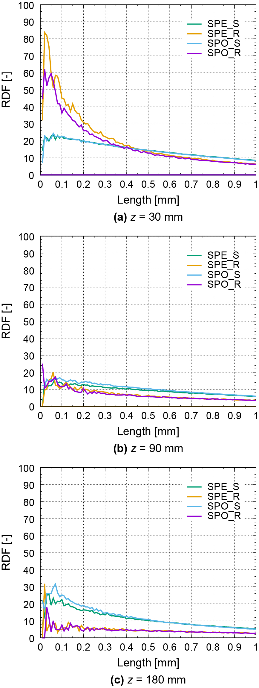
Variation of RDF in characteristic length scale for (a) z = 30 mm, (b) z = 90 mm (c) z = 180 mm. Reprinted with permission from Ref. (Zhang et al., 2018b). Copyright: (2018) Elsevier B.V.

5. Conclusions

This paper describes the reviews of the recent works in the analysis, modeling, and simulation of the motion of a non-spherical particle. The motions of the non-spherical pulverized coal, sphere, and spheroidal particles were analyzed in detail by means of the fully resolved DNS of the six-degree of freedom particle motion by employing the ALE method. It was found that the motion of pulverized coal particle can be reproduced by the spheroidal particle with the equivalent volume. From the detailed analysis of the motion of the spheroidal particle, it was revealed that the PDF of the sine curve can capture the variation of the drag coefficient due to the particle oscillation and rotation.

The motion model based on the six-degree of freedom motion DNS was applied to the particle dispersion simulation in an isotropic turbulent flow by mean of the point mass approximation DNS. The results showed that the effect of the particle shape was clearly observed in the characteristics of the particle dispersion by evaluating the D number and RDF. It was found that the non-spherical particle’s representative Stokes number becomes larger as the sphericity increases.

Furthermore, the proposed motion model was applied to the LES of particle dispersion in an axial jet flow and validated by comparing it with the experimental data. It was revealed that the effects of the particle size distribution and the shape observed in the experiment were precisely captured by the LES that coincided with the trend found in the isotropic turbulent flow.

Acknowledgements

This study was partly supported by JSPS KAKENHI Grant No. 25420173 and 16K06125, and a grant from the Information Center of Particle Technology, Japan. HW is grateful to Dr. Kazuki Tainaka of CRIEPI for his great support to conduct the PIV measurement in the experiment.

References

•  Ahn  S.,  Watanabe  H.,  Kitagawa  T., Numerical investigation on the detailed structure of a coaxial coal jet flame using large-eddy simulation with elementary reactions, Energy and Fuels, 33 (2019) 4621–4631. DOI:10.1021/acs.energyfuels.9b00734
•  Broday  D.,  Fichman  M.,  Shapiro  M.,  Gutfinger  C., Motion of spheroidal particles in vertical shear flows, Physics of fluids, 10 (1998) 86–100. DOI:10.1063/1.869552
•  Clift  R.,  Grace  J.R.,  Weber  M.E., Bubbles, Drops, and Particles, Academic Press, 1978, ISBN: 9780121769505.
•  Crowe  C.T.,  Sharma  M.P.,  Stock  D.E., The particle-source-in cell (PSI-CELL) model for gas-droplet flows, Journal of Fluids Engineering, 99 (1977) 325–332. DOI:10.1115/1.3448756
•  Feng  J.,  Joseph  D.D.,  Glowinski  R.,  Pan  T.W., A three-dimensional computation of the force and torque on an ellipsoid settling slowly through a viscoelastic fluid, Journal of Fluid Mechanics, 25 (1995) 1–16. DOI:10.1017/S0022112095002217
•  Fessler  J.R.,  Kulick  J.D.,  Eaton  J.K., Preferential concentration of heavy particles in a turbulent channel flow, Physics of Fluids, 6 (1994) 3742–3749. DOI:10.1063/1.868445
•  Haider  A.,  Levenspiel  O., Drag coefficient and terminal velocity of spherical and nonspherical particles, Powder Technology, 58 (1989) 63–70. DOI:10.1016/0032-5910(89)80008-7
•  Hashimoto  N.,  Watanabe  H., Numerical analysis on effect of furnace scale on heat transfer mechanism of coal particles in pulverized coal combustion field, Fuel Processing Technology, 145 (2016) 20–30. DOI:10.1016/j.fuproc.2016.01.024
•  Hirt  C.W.,  Amsden  A.A.,  Cook  J.L., An arbitrary Lagrangian-Eulerian computing method for all flow speeds, Journal of Computational Physics, 14 (1974) 227–253. DOI:10.1016/0021-9991(74)90051-5
•  Holzer  A.,  Sommerfeld  M., New simple correlation formula for the drag coefficient of non-spherical particles, Powder Technology, 184 (2008) 361–365. DOI:10.1016/j.powtec.2007.08.021
•  Kurose  R.,  Watanabe  H.,  Makino  H., Numerical simulation of pulverized coal combustion, KONA Powder and Particle Journal, 27 (2009) 144–156. DOI:10.14356/kona.2009014
•  Moin  P.,  Squires  K.,  Cabot  W.,  Lee  S., A dynamic subgrid-scale model for compressible turbulence and scalar transport, Physics of Fluids A: Fluid Dynamics, 3 (1991) 2746–2757. DOI:10.1063/1.858164
•  Mordant  R.,  Pinton  J.-F., Velocity measurement of a settling sphere, European Physical Journal B, 18 (2000) 343–352. DOI:10.1007/PL00011074
•  Mortensen  P.H.,  Andersson  H.I.,  Gillissen  J.J.J.,  Boersma  B.J., On the orientation of ellipsoidal particles in a turbulent shear flow, International Journal of Multiphase Flow, 34 (2008) 678–683. DOI:10.1016/j.ijmultiphaseflow.2007.12.007
•  Muto  M.,  Tsubokura  M.,  Oshima  N., Negative magnus lift on a rotating sphere at around the critical Reynolds number, Physics of Fluids, 24 (2012), 014102. DOI:10.1063/1.3673571
•  Muto  M.,  Watanabe  H.,  Kurose  R., Large eddy simulation of pulverized coal combustion in multi-burner system—effect of in-furnace blending method on NO emission—, Advanced Powder Technology, 30 (2019) 3153–3162. DOI:10.1016/j.apt.2019.09.024
•  Ooi  A.,  Martin  J.,  Soria  J.,  Chong  M.S., A study of the evolution and characteristics of the invariants of the velocity-gradient tensor in isotropic turbulence, Journal of Fluid Mechanics, 381 (1999) 141–174. DOI:10.1017/S0022112098003681
•  Rosendahl  L., Using a multi-parameter particle shape description to predict the motion of non-spherical particle shapes in swirling flow, Applied Mathematical Modelling, 24 (2000) 11–25. DOI:10.1016/S0307-904X(99)00023-2
•  Schlichting  H.,  Gersten  K.,  Krause  E.,  Oertel  H., Boundary-layer Theory, Vol. 7, Springer (1955), ISBN 0-07-055334-3.
•  Watanabe  H.,  Otaka  M., Numerical simulation of coal gasification in entrained flow coal gasifier, Fuel, 85 (2006) 1935–1943. DOI:10.1016/j.fuel.2006.02.002
•  Watanabe  H.,  Kurose  R., Modeling and simulation of coal gasification on an entrained flow coal gasifier, Advanced Powder Technology, 31 (2020) 2733–2741. DOI:10.1016/j.apt.2020.05.002
•  Watanabe  H.,  Tanno  K.,  Umetsu  H.,  Umemoto  S., Modeling and simulation of coal gasification on an entrained flow coal gasifier with a recycled CO₂ injection, Fuel, 142 (2015) 250–259. DOI:10.1016/j.fuel.2014.11.012
•  Zastawny  M.,  Mallouppas  G.,  Zhao  F.,  van Wachem  B., Derivation of drag and lift force and torque coefficients for non-spherical particles in flows, International Journal of Multiphase Flow, 39 (2012) 227–239. DOI:10.1016/j.ijmultiphaseflow.2011.09.004
•  Zhang  W.,  Tainaka  K.,  Ahn  S.,  Watanabe  H.,  Kitagawa  T., Experimental and numerical investigation of effect of particle shape and size distribution on particles’ dispersion in a coaxial jet flow, Advanced Powder Technology, 29 (2018a)2322–2330. DOI: 10.1016/j.apt.2018.06.008
•  Zhang  W.,  Watanabe  H.,  Kitagawa  T., Numerical investigation of effects of particle shape on dispersion in an isotropic turbulent flow, Advanced Powder Technology, 29 (2018b)2048–2060. DOI:10.1016/j.apt.2018.05.011

Nomenclature

DNS

Direct numerical simulation

LES

Large-eddy simulation

PIV

Particle image velocimetry

RANS

Reynolds-averaged Navier-Stokes simulation

SGS

Subgrid scale

A

projection area of particle (m²)

C_D

drag coefficient

d

particle size (m)

D

D number (−)

F

force acting on particle (kg m s⁻²)

g

gravity (m s⁻²), radial distribution function

l

length (m)

m

particle mass (kg)

N_p

total number of particle pairs (−)

p

pressure (Pa)

r

distance of particle pairs (m)

Re

Reynolds number (−)

St

Stokes number (−)

t

time (s)

u

fluid velocity (m s⁻¹)

u′

mesh velocity (m s⁻¹)

V

volume of domain (m³)

V_p

particle volume (m³)

υ

particle velocity (m s⁻¹)

ϕ

sphericity (−)

η

Kolmogorov length scale (m)

λ

mean number of particles (−)

μ

gas viscosity (Pa s)

ρ_f

gas density (kg m⁻³)

ρ_p

particle density (kg m⁻³)

σ

stress tensor, standard deviation

σ_Poi

standard deviation of Poisson distribution

τ_p

particle response time (s)

Authors’ Short Biographies

Hiroaki Watanabe

Prof. Hiroaki Watanabe received his Ph.D. from Kyoto University in 2008. He worked as a researcher at Central Research Institute of Electric Power Industry from 1998 to 2014. He joined Department of Mechanical Engineering at Kyushu University as an Associate Professor in 2014 and became a Full Professor of Department of Advanced Environmental Science and Engineering in 2020. His research interest is mathematical modeling and simulation of multiphase turbulent reacting flows. Modeling of co-combustion of solid carbon fuels with carbon-free gaseous fuels is currently being examined.

Wei Zhang

Dr. Zhang Wei received his Ph.D. from Kyushu University in 2017 and then worked as a doctoral researcher at Kyushu University for half a year. He moved to Nagoya University and worked as a designated Assistant Professor from 2018 to 2020. Now he is a Lecturer working in the College of Mechanical and Transportation Engineering, China University of Petroleum-Beijing. He mainly works on the numerical simulation of gas-solid multiphase reacting flows for carbon conversion, such as the CO₂ methanation, and the gasification of carbon fuels including coal, biomass, and petroleum coke.