Image and Spectral Processing for ToF-SIMS Analysis of Biological Materials

Abstract

Time-of-flight secondary ion mass spectrometry (ToF-SIMS) instruments can rapidly produce large complex data sets. Within each spectrum, there can be hundreds of peaks. A typical 256×256 pixel image contains 65,536 spectra. If this is extended to a 3D image, the number of spectra in a given data set can reach the millions. The challenge becomes how to process these large data sets while taking into account the changes and differences between all the peaks in the spectra. This is particularly challenging for biological materials that all contain the same types of proteins and lipids, just in varying concentrations and spatial distributions. This data analysis challenge is further complicated by the limitations in the ion yield of higher mass, more chemically specific species, and potentially by the processing power of typical computers. Herein we briefly discuss analysis methodologies including univariate analysis, multivariate analysis (MVA) methods, and some of the limitations of ToF-SIMS analysis of biological materials.

INTRODUCTION

Time-of-flight secondary ion mass spectrometry (ToF-SIMS) generates an information rich yet complex set of spectra. A typical spectrum can contain hundreds to thousands of peaks. With the advent of 2D and 3D imaging in modern ToF-SIMS instruments, one can quickly acquire an enormous amount of data. For example a 2D 256×256 pixel image contains 65,536 spectra. If this is extended to a 3D image, the number of spectra can increase to the millions depending on the number of 2D images acquired during the analysis. The challenge then becomes how to efficiently process and analyze this data in order to extract the pertinent information and gain insight about the sample.

When analyzing biological materials (cells, tissues, etc.), the analyst is presented with the additional challenges of low ion yields and the lack of molecular specificity of many of the resulting peaks.^1–3) Low ion yields are the result of the low ionization efficiencies of ToF-SIMS. Typically less than 1% of the material removed from the surface during the primary ion bombardment is ionized. This can be particularly problematic if the analyte of interest is already present at low concentrations at the surface.

Major components present in cells and tissues include proteins and lipids. ToF-SIMS analysis of proteins has been shown to generate mainly fragments of the 20 component amino acids, and not large fragments or even small peptides. It has been shown that the relative intensity of these amino acid fragments encodes information about the protein’s composition,^4–8) conformation^9–13) and orientation.^14–17) However, it would be challenging to determine the identity of individual proteins in a complex mixture such as is found in cells or tissues using ToF-SIMS.⁸⁾ Many nice examples of lipid analysis with ToF-SIMS have been shown.^3,18–25) Control spectra for many common lipids have been published and used to study cells and tissues.^3,19,26) However, many of the higher mass, more chemically specific, lipid peaks are not detected, especially when one collects high spatial resolution images using ToF-SIMS. This is partially due to low primary ion currents and adjustments required to the analyzer when using the high spatial resolution settings on current ToF-SIMS systems. The need for these different settings is due to the fact that most modern ToF-SIMS instruments utilize a pulsed primary ion source that can either be optimized for high mass resolution or high spatial resolution, but not both at the same time. The J105 instrument is an exception to this rule as it uses a DC primary ion beam and therefore is capable of collecting high spatial resolution images with good mass resolution.^27,28) Even with this advantage, the J105 is still limited by low ion yields from biological materials.

In spite of these limitations, significant work has been done in the analysis of biological materials with ToF-SIMS.^{1,3–5,8,18–21,23–26,28–50)} For this work, ToF-SIMS analysts have used a variety of methods to process and understand their data. These include a combination of traditional manual analysis and the application of multivariate analysis (MVA) methods. In this manuscript, we briefly overview the current data processing methods available for the ToF-SIMS analyst, outline some of the challenges faced for ToF-SIMS analysis of biological materials, and summarize some of the needs to continue to move ToF-SIMS analysis of biological materials to the next level.

CURRENT PRACTICES

ToF-SIMS is a mass spectrometry technique, and as such involves basic mass spectrometry analysis methods such as spectral calibration, peak identification, integration of peak areas, and plotting of peak intensity maps for imaging. The most basic analysis involves searching through the spectra to locate expected peaks from a known component, or identifying dominant peaks to determine the structure of unknown components. Often peak area ratios are created to track changes in chemistry across a set of samples. Other basic analysis methods for imaging include creating region of interest (ROI) spectra from a given region within an image, or creating peak area images from a given peak or set of peaks. These methods can be useful to highlight some differences between the samples, however, focusing on individual peaks or ROIs risks adding user bias to the analysis and ignores the potential information present across the rest of the spectra. To avoid this problem and take advantage of all of the data, many users apply MVA methods to ToF-SIMS spectra and images.^22,51–56) Though there is still a fair amount of exploration of new MVA methods, in general the main methods used for processing ToF-SIMS data include principal components analysis (PCA), partial least squares (PLS), multivariate curve resolution (MCR), and maximum autocorrelation factors (MAF). Herein we provide an example of ToF-SIMS analysis of mouse muscle tissue using manual analysis, PCA and MCR to illustrate the strengths and weaknesses of the data processing methods and of the ToF-SIMS instrumentation.

ToF-SIMS image analysis of mouse muscle tissue

ToF-SIMS imaging of mouse muscle tissue was carried out using an Iontof 5-100 instrument equipped with a 25 kV bismuth primary ion source and a 10 kV C₆₀ sputter source. A positive ion image was acquired by summing the signal from 150 sequential analysis cycles using a 200 micron×200 micron raster with Bi₃⁺ at 0.05 pA (∼1.5×10¹⁰ ions/cm²) for imaging, followed by a 10 second sputter of a 500 micron×500 micron area using C₆₀⁺⁺ at 0.45 nA (∼1.1×10¹³ ions/cm²). This summation protocol was used to increase the signal to noise within the image and to acquire the image data over a thickness of the tissue that would be more comparable with future optical microscopy analysis. The approximate depth of the summed image was 1.5 microns.

The image data was processed using standard manual analysis of peak area images and by MVA using PCA and MCR. For MVA, all peaks above background were selected and peak area images were generated using the Iontof software (Iontof, Münster, Germany). The image data was exported using the iontof .bif6 file format and then imported into the NESAC/BIO Imagegui (NBtoolbox, NESAC/BIO, University of Washington, http://mvsa.nb.uw.edu/) within Matlab (Mathworks, Natick, MA). MCR was carried out using the MCR-ALS gui (Roma Tauler and Anna de Juan, University of Barcelona, http://www.mcrals.info/) accessed through the Imagegui. PCA and MCR were carried out using the Poisson scaled^57,58) and mean centered data. PCA scores were used as initial estimates for the MCR analysis. An explanation of PCA and MCR are beyond the scope of this manuscript. Good overviews of each method can be found in the literature.^{22,51,53,55,59–64)} Briefly, PCA looks for the major directions of variance within the data. For PCA processing of ToF-SIMS image data, this results in finding which areas of the image are chemically distinct, and which peaks are responsible for the differences among those areas. The output from PCA is a set of score images and peak loadings. Within these plots, positive scores are shown as brighter regions and correspond with positive loadings. Negative scores are shown as darker regions and correspond with negative loadings. MCR uses an alternating least squares routine to find a set of “pure” components that describe the differences within the data set. MCR was carried out using a non-negativity constraint meaning that the resulting components are restricted to positive values. This means for the MCR component images, the brighter regions show higher intensity of the peaks shown in the component spectra, whereas darker regions show areas of lower or no intensity for those peaks.

Figure 1 shows a series of peaks selected manually by browsing through the full data set. Peaks were randomly selected that showed representative images of the patterns seen within the data. As seen in the figure, peaks could be found that are representative of the muscle cell nuclei (top row Fig. 1), the cell bodies (middle row Fig. 1), and the intercellular regions (bottom row Fig. 1). This manual analysis is fairly quick and allows one to pick out peaks of interest, however it brings definite user bias to the analysis since the analyst chooses which peaks to focus on and present.

Fig. 1. ToF-SIMS peak area images for manually selected peaks.

Top row (left to right) m/z=63, 79, 181. Middle row (left to right) m/z=33, 59, 71. Bottom row (left to right) m/z=65, 91, 107. All images are 200 micron×200 micron. The scale bars shown are 20 microns.

Figures 2–4 show the first 3 principal components (PC) from PCA. As seen in the figures, similar features as were seen in the manual analysis can be seen in the PC score images. However with PCA all of the peaks that show the same trends are found without the need of user input. As would be expected, the peaks selected in the manual analysis are found to correspond to their respective areas within the scores and loadings plots. For example, the nuclei are highlighted in the PC1 scores plot (bright areas) and are seen to correspond with peaks such as m/z 63, 79, and 181 all of which were chosen in the manual analysis. In addition several other peaks are shown to have positive loadings on PC1. These peaks show similar spatial distribution as the m/z 63, 79, and 181 peaks, with a higher relative intensity from the nuclei of the cells (data not shown). Similar trends can be seen for PC2 and PC3 where PCA highlights peaks that show the same relative intensity patterns.

Fig. 2. PCA PC 1 scores from the mouse muscle data.

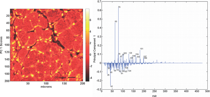
PCA scores (left) and loadings (right) from the mouse muscle data. PC1 is shown to separate the cell nuclei (positive scores–bright regions) from the intercellular spaces and cell bodies (negative scores–darker regions).

Fig. 3. PCA PC2 scores from the mouse muscle data.

PCA scores (left) and loadings (right) from the mouse muscle data. PC2 is shown to separate the cell bodies and some cell edges (positive scores–bright regions) from the cell nuclei and intercellular spaces (negative scores–darker regions).

Fig. 4. PCA PC3 scores from the mouse muscle data.

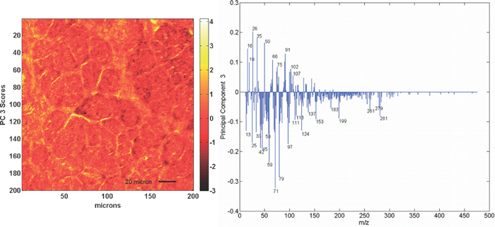
PCA scores (left) and loadings (right) from the mouse muscle data. PC3 is shown to separate areas of the cell bodies and some cell edges (positive scores–bright regions) from other areas of the cell bodies (negative scores–darker regions).

One can go through the scores and loadings plots and quickly summarize the trends in the data. However, it is noted that many of the same peaks have relatively high loadings across multiple PCs. Looking at the loadings, one can see that the trends are mostly self consistent. For example the m/z 63, 79, and 181 peaks are always seen to correspond with the nuclei of the cells and the m/z 42 peak is seen to correspond with the cell body and intercellular space. However, the trends in some of the peaks are not as clear. For example, the peak at m/z 91 appears to correspond with the intercellular areas in the PC1 and PC2 scores images, but for PC3 it shows a positive loading that would correspond with the bright lines in the image. Based on their location, these lines could be intercellular regions or could be on the edges of the muscle cells.

Some analysts find PCA to be somewhat confusing due to the fact that peaks can be present in multiple PCs, and that PCA produces both positive and negative scores and loadings. This and the desire to try to resolve the data into “pure” components has led some users to apply MCR processing to their ToF-SIMS data. It is typical to use the PCA scores as an initial guess for the number of “pure” components for MCR, which means that MCR and PCA provide the same information, but present it differently. This is important to note because if there is no clear indication of chemically different regions in PCA, it is unlikely that MCR will find a logical answer. It may come up with a set of components, but they may not be chemically relevant or real. In fact, it is typical that the trends seen in MCR will also be apparent from PCA, but that MCR will present them in a visually simpler format. Figures 5–7 show the 3 MCR components calculated when using the 3 PC model from PCA as the initial guess. As seen in the figure, MCR separates the nuclei, the cell bodies and the intercellular space in the 3 component images. It is noted that component 3 also shows some contrast with the cell bodies in the lower half of the image. This appears to be highlighting a chemical difference between the different muscle cells. Figure 8 shows an RGB overlay of the three MCR component images. Very little overlap is seen within the image as seen by the lack of colors other than pure red, green, and blue. It is noted that the differences in the signal from the cell bodies are not due to differences in ion yields due to instrumentation or charging, as normalizing the data to the total intensity of each pixel does not change the general trends seen in the data (data not shown).

Fig. 5. MCR component 1 data from the mouse muscle sample.

MCR component image (left) and component spectra (right) from the mouse muscle data. MCR component 1 is shown to highlight the cell nuclei. The peaks in the spectra are mainly attributable to phosphate fragments and phosphate salts.

Fig. 6. MCR component 2 data from the mouse muscle sample.

MCR component image (left) and component spectra (right) from the mouse muscle data. MCR component 2 is shown to highlight the cell bodies. Some variation in the relative intensity of the cell bodies is seen across the image.

Fig. 7. MCR component 3 data from the mouse muscle sample.

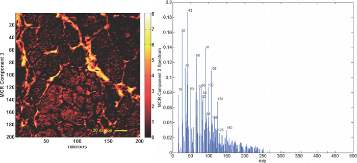
MCR component image (left) and component spectra (right) from the mouse muscle data. MCR component 3 is shown to highlight intercellular space and some of the cell bodies.

Fig. 8. RGB overlay of MCR component images.

Red=Component 1, Green=Component 2, Blue=Component 3.

Comparing the PCA and MCR results, one can see that MCR component 1 and the positive scores from PC1 clearly highlight the cell nuclei. The PC1 positive loadings and MCR component 1 spectra look almost identical. Similar trends can be seen where MCR component 2 is seen to correspond well with the PC3 negative scores and loadings and MCR component 3 is seen to correspond well with the PC2 negative scores and loadings. This is not unexpected since the MCR results are based off the initial guess of 3 components from the PCA scores, and because both methods are looking at the variance within the data set that is caused by the differences in the relative intensities of the same peaks.

It should be noted that it is not possible to say which analysis method is better than the other. Which method is used will depend on the goals of the analysis. For some systems, a simple manual analysis of certain components with known secondary ion peaks may be sufficient. The various MVA methods are simply tools that enable the user to analyze the full ToF-SIMS data matrix and minimize user bias. PCA is a good choice for general data exploration and sometimes may be all that is required to summarize important features and trends in a data set. It is also important to remember that each MVA method carries a set of assumptions and many are dependent on the data scaling or initial guesses used.⁶⁴⁾ For example, the results from MCR will depend significantly on the number of components assumed in the initial estimate. For a more in depth discussion of the various MVA methods and their application to ToF-SIMS data the reader is referred to the current literature.^22,51–56)

LIMITATIONS AND NEEDS

One thing that can be seen from the data presented in this study is that all of the peaks highlighted in the PCA and MCR analysis were relatively low mass peaks (<300 m/z). This is due to the low ion yields for high mass peaks (>300 m/z). Although one can extract information about a given sample set from analyzing the relative intensity differences of the low mass peaks, to get more chemically specific information from biological samples higher intensities of higher mass peaks are required. This is particularly true for high spatial resolution imaging where count rates of the high mass peaks are significantly lower. Thus any improvements in secondary ion yields that results from advances in new instrumentation (ions sources, detectors, etc.) and sample preparation (e.g., matrix enhanced SIMS) would provide a direct benefit for ToF-SIMS analysis of biological materials.

Even when high mass peaks can be detected, the challenge in many cases is to determine the peak identity. This can be particularly challenging for high mass peaks where the number of possible matches to a given mass can reach the thousands. Some work has been done to identify peaks related to amino acids,^65,66) DNA bases,⁶⁷⁾ and lipids,³⁾ however there is still a lack of easily accessible databases of ToF-SIMS data that one can use to help identify peaks of interest. It is not clear how this type of database should be organized or started, but the presence of such a database would be useful to the community.

Although this paper concentrated on 2D ToF-SIMS image data, the increased use of 3D data sets presents the challenge of needing increased computing power. This is a more easily addressable challenge, since it is relatively easy to purchase a computer with sufficient computing power for a reasonable price. It should be noted that this does not mean one can use a standard off the shelf system to easily process large data sets. Modern computers will do fine for most 2D data sets, however when moving to 3D analysis the user must significantly increase the computing power of their system or develop more efficient algorithms for processing the 3D data sets. Though we do not provide specific computer system recommendations since those will depend on the specific needs of the user and the data sets being processed, we do recommend that the user install the maximum amount of RAM possible for their system and choose a system with the fastest processor available. Multi-core processors are highly recommended. It is also recommended that the user install a dedicated graphics card equipped with the maximum amount of on board RAM. Furthermore, to more efficiently process the increasingly large data sets generated by ToF-SIMS, it is recommended that programs be developed which take advantage of the parallel processing capabilities provided by modern graphics cards equipped with multi-core GPUs.

CONCLUSION

ToF-SIMS analysis of biological materials has been shown to be an effective method to extract useful chemical information from a wide variety of samples. ToF-SIMS can be used for a wide range of sample types, and the current instrumentation allows analysis of samples in both the frozen hydrated and dehydrated states. MVA methods have enabled the analysis of full data sets that eliminates user bias and allows access to information from all generated peaks. This has enabled the analysis of many types of samples and produced useful information. However, there are still limitations that need to be overcome. These include the need for increased ion yields of high mass, chemically specific peaks, the generation of and access to databases of spectra from biologically relevant materials that can be used for peak identification, and the need for more efficient programs that take advantage of multi-core, multi-threaded GPU graphics cards.

Acknowledgment

The authors gratefully acknowledge the funding and facilities provided by the National ESCA and Surface Analysis Center for Biomedical Problems (NESAC/BIO) through grant EB-002027 from the National Institutes of Health. The authors also thank Dr. Nick Whitehead for providing the mouse muscle samples used for the ToF-SIMS image processing examples in this study.

REFERENCES

• 1)  J. S. Fletcher, A. Henderson, G. X. Biddulph, S. Vaidyanathan, N. P. Lockyer, J. C. Vickerman. Uncovering new challenges in bio-analysis with ToF-SIMS. Appl. Surf. Sci. 255: 1264–1270, 2008.
• 2)  J. C. Vickerman. Molecular Surface Mass Spectrometry by SIMS. in Surface Analysis—The Principal Techniques 2nd Ed. (Ed: J. C. Vickerman, I. S. Gilmore), John Wiley & Sons, Chichester, 2009, pp. 113–205.
• 3)  M. K. Passarelli, N. Winograd. Lipid imaging with time-of-flight secondary ion mass spectrometry (ToF-SIMS). Biochim. Biophys. Acta 1811: 976–990, 2011.
• 4)  M. S. Wagner, M. Shen, T. A. Horbett, D. G. Castner. Quantitative time-of-flight secondary ion mass spectrometry for the characterization of multicomponent adsorbed protein films. Appl. Surf. Sci. 203–204: 704–709, 2003.
• 5)  M. S. Wagner, M. Shen, T. A. Horbett, D. G. Castner. Quantitative analysis of binary adsorbed protein films by time of flight secondary ion mass spectrometry. J. Biomed. Mater. Res. A 64: 1–11, 2003.
• 6)  M. S. Wagner, S. L. McArthur, M. Shen, T. A. Horbett, D. G. Castner. Limits of detection for time of flight secondary ion mass spectrometry (ToF-SIMS) and X-ray photoelectron spectroscopy (XPS): Detection of low amounts of adsorbed protein. J. Biomater. Sci. Polym. Ed. 13: 407–428, 2002.
• 7)  S. Ferrari, B. D. Ratner. ToF-SIMS quantification of albumin adsorbed on plasma-deposited fluoropolymers by partial least-squares regression. Surf. Interface Anal. 29: 837–844, 2000.
• 8)  M. S. Wagner, T. A. Horbett, D. G. Castner. Characterizing multicomponent adsorbed protein films using electron spectroscopy for chemical analysis, time-of-flight secondary ion mass spectrometry, and radiolabeling: Capabilities and limitations. Biomaterials 24: 1897–1908, 2003.
• 9)  I. M. Kempson, A. L. Martin, J. A. Denman, P. W. French, C. A. Prestidge, T. J. Barnes. Detecting the presence of denatured human serum albumin in an adsorbed protein monolayer using TOF-SIMS. Langmuir 26: 12075–12080, 2010.
• 10)  M. Henry, C. Dupont-Gillain, P. Bertrand. Conformation change of albumin adsorbed on polycarbonate membranes as revealed by ToF-SIMS. Langmuir 19: 6271–6276, 2003.
• 11)  N. Xia, D. G. Castner. Preserving the structure of adsorbed protein films for time-of-flight secondary ion mass spectrometry analysis. J. Biomed. Mater. Res. A 67: 179–190, 2003.
• 12)  N. Xia, C. J. May, S. L. McArthur, D. G. Castner. Time-of-flight secondary ion mass spectrometry analysis of conformational changes in adsorbed protein films. Langmuir 18: 4090–4097, 2002.
• 13)  T. Mouhib, A. Delcorte, C. Poleunis, M. Henry, P. Bertrand. C₆₀ SIMS depth profiling of bovine serum albumin protein coating films: A conformational study. Surf. Interface Anal. 42: 641–644, 2010.
• 14)  J.-W. Park, I.-H. Cho, D. W. Moon, S.-H. Paek, T. G. Lee. ToF-SIMS and PCA of surface-immobilized antibodies with different orientations. Surf. Interface Anal. 43: 285–289, 2011.
• 15)  L. Baugh, T. Weidner, J. E. Baio, P.-C. T. Nguyen, L. J. Gamble, P. S. Stayton, D. G. Castner. Probing the orientation of surface-immobilized protein G B1 using ToF-SIMS, sum frequency generation, and NEXAFS spectroscopy. Langmuir 26: 16434–16441, 2010.
• 16)  H. Wang, D. G. Castner, B. D. Ratner, S. Y. Jiang. Probing the orientation of surface-immobilized immunoglobulin G by time-of-flight secondary ion mass spectrometry. Langmuir 20: 1877–1887, 2004.
• 17)  F. Liu, M. Dubey, H. Takahashi, D. G. Castner, D. W. Grainger. Immobilized antibody orientation analysis using secondary ion mass spectrometry and fluorescence imaging of affinity-generated patterns. Anal. Chem. 82: 2947–2958, 2010.
• 18)  M. C. Biesinger, D. J. Miller, R. R. Harbottle, F. Possmayer, N. S. McIntyre, N. O. Petersen. Imaging lipid distributions in model monolayers by ToF-SIMS with selectively deuterated components and principal components analysis. Appl. Surf. Sci. 252: 6957–6965, 2006.
• 19)  C. R. Anderton, B. Vaezian, K. Lou, J. F. Frisz, M. L. Kraft. Identification of a lipid-related peak set to enhance the interpretation of TOF-SIMS data from model and cellular membranes. Surf. Interface Anal. 44: 322–333, 2012.
• 20)  S. L. McArthur, M. W. Halter, V. Vogel, D. G. Castner. Covalent coupling and characterization of supported lipid layers. Langmuir 19: 8316–8324, 2003.
• 21)  B. Vaezian, C. R. Anderton, M. L. Kraft. Discriminating and imaging different phosphatidylcholine species within phase-separated model membranes by principal component analysis of TOF-secondary ion mass spectrometry images. Anal. Chem. 82: 10006–10014, 2010.
• 22)  J. L. S. Lee, I. S. Gilmore. The Application of Multivariate Data Analysis Techniques in Surface Analysis. in Surface Analysis —The Principal Techniques, 2nd Ed. (Ed: J. C. Vickerman, I. S. Gilmore), John Wiley & Sons, Chichester, 2009, pp. 563–611.
• 23)  M. J. Baker, L. Zheng, N. Winograd, N. P. Lockyer, J. C. Vickerman. Mass spectral imaging of glycophospholipids, cholesterol, and glycophorin A in model cell membranes. Langmuir 24: 11803–11810, 2008.
• 24)  P. D. Piehowski, A. M. Davey, M. E. Kurczy, E. D. Sheets, N. Winograd, A. G. Ewing, M. L. Heien. Time-of-flight secondary ion mass spectrometry imaging of subcellular lipid heterogeneity: Poisson counting and spatial resolution. Anal. Chem. 81: 5593–5602, 2009.
• 25)  M. K. Passarelli, N. Winograd. Characterizing in situ glycerophospholipids with SIMS and MALDI methodologies. Surf. Interface Anal. 43: 269–271, 2011.
• 26)  S. Parry, N. Winograd. High-resolution TOF-SIMS imaging of eukaryotic cells preserved in a trehalose matrix. Anal. Chem. 77: 7950–7957, 2005.
• 27)  S. Rabbani, J. S. Fletcher, N. P. Lockyer, J. C. Vickerman. Exploring subcellular imaging on the buncher-ToF J105 3D chemical imager. Surf. Interface Anal. 43: 380–384, 2011.
• 28)  J. S. Fletcher, S. Rabbani, A. Henderson, N. P. Lockyer, J. C. Vickerman. Three-dimensional mass spectral imaging of HeLa-M cells—Sample preparation, data interpretation and visualisation. Rapid Commun. Mass Spectrom. 25: 925–932, 2011.
• 29)  M. Brulet, A. Seyer, A. Edelman, A. Brunelle, J. Fritsch, M. Ollero, O. Laprévote. Lipid mapping of colonic mucosa by cluster TOF-SIMS imaging and multivariate analysis in cftr knockout mice. J. Lipid Res. 51: 3034–3045, 2010.
• 30)  L. Wu, J. S. Felton, K. J. Wu. Applying imaging ToF-SIMS and PCA in differentiation of tissue types. Methods Mol. Biol. 656: 267–281, 2010.
• 31)  C. Brüning, S. Hellweg, S. Dambach, D. Lipinsky, H. F. Arlinghaus. Improving the interpretation of ToF-SIMS measurements on adsorbed proteins using PCA. Surf. Interface Anal. 38: 191–193, 2006.
• 32)  J. Wald, C. Müller, M. Wahl, W. Hoth‐Hannig, M. Hannig, M. Kopnarski, C. Ziegler. ToF-SIMS investigations of adsorbed proteins on dental titanium. Phys. Status Solidi 207: 831–836, 2010.
• 33)  S. Vaidyanathan, J. S. Fletcher, R. M. Jarvis, A. Henderson, N. P. Lockyer, R. Goodacre, J. C. Vickerman. Explanatory multivariate analysis of ToF-SIMS spectra for the discrimination of bacterial isolates. Analyst (Lond.) 134: 2352–2360, 2009.
• 34)  J. Mains, C. Wilson, A. Urquhart. ToF-SIMS analysis of ocular tissues reveals biochemical differentiation and drug distribution. Eur. J. Pharm. Biopharm. 79: 328–333, 2011.
• 35)  M. J. Baker, E. Gazi, M. D. Brown, N. W. Clarke, J. C. Vickerman, N. P. Lockyer. ToF-SIMS PC-DFA analysis of prostate cancer cell lines. Appl. Surf. Sci. 255: 1084–1087, 2008.
• 36)  S. Vaidyanathan, J. S. Fletcher, A. Henderson, N. P. Lockyer, J. C. Vickerman. Exploratory analysis of TOF-SIMS data from biological surfaces. Appl. Surf. Sci. 255: 1599–1602, 2008.
• 37)  K. R. Amaya, J. V. Sweedler, D. F. Clayton. Small molecule analysis and imaging of fatty acids in the zebra finch song system using time-of-flight-secondary ion mass spectrometry. J. Neurochem. 118: 499–511, 2011.
• 38)  J. S. Fletcher. Cellular imaging with secondary ion mass spectrometry. Analyst (Lond.) 134: 2204–2215, 2009.
• 39)  J. C. Ingram, W. F. Bauer, R. M. Lehman, S. P. O’Connell, A. D. Shaw. Detection of fatty acids from intact microorganisms by molecular beam static secondary ion mass spectrometry. J. Microbiol. Methods 53: 295–307, 2003.
• 40)  C. A. Barnes, J. Brison, M. Robinson, D. J. Graham, D. G. Castner, B. D. Ratner. Identifying individual cell types in heterogeneous cultures using secondary ion mass spectrometry imaging with C₆₀ etching and multivariate analysis. Anal. Chem. 84: 893–900, 2012.
• 41)  H. E. Canavan, D. J. Graham, X. H. Cheng, B. D. Ratner, D. G. Castner. Comparison of native extracellular matrix with adsorbed protein films using secondary ion mass spectrometry. Langmuir 23: 50–56, 2007.
• 42)  H. E. Canavan, X. H. Cheng, D. J. Graham, B. D. Ratner, D. G. Castner. Cell sheet detachment affects the extracellular matrix: A surface science study comparing thermal liftoff, enzymatic, and mechanical methods. J. Biomed. Mater. Res. A 75: 1–13, 2005.
• 43)  H. E. Canavan, X. H. Cheng, D. J. Graham, B. D. Ratner, D. G. Castner. Surface characterization of the extracellular matrix remaining after cell detachment from a thermoresponsive polymer. Langmuir 21: 1949–1955, 2005.
• 44)  K. S. Kulp, E. S. F. Berman, M. G. Knize, D. L. Shattuck, E. J. Nelson, L. Wu, J. L. Montgomery, J. S. Felton, K. J. Wu. Chemical and biological differentiation of three human breast cancer cell types using time-of-flight secondary ion mass spectrometry. Anal. Chem. 78: 3651–3658, 2006.
• 45)  L. Wu, X. Lu, K. S. Kulp, M. G. Knize, E. S. F. Berman, E. J. Nelson, J. S. Felton, K. J. J. Wu. Imaging and differentiation of mouse embryo tissues by ToF-SIMS. Int. J. Mass. 260(Spec.): 137–145, 2007.
• 46)  A. M. Belu, D. J. Graham, D. G. Castner. Time-of-flight secondary ion mass spectrometry: Techniques and applications for the characterization of biomaterial surfaces. Biomaterials 24: 3635–3653, 2003.
• 47)  M. E. Kurczy, P. D. Piehowski, S. A. Parry, M. Jiang, G. Chen, A. G. Ewing, N. Winograd. Which is more important in bioimaging SIMS experiments—The sample preparation or the nature of the projectile? Appl. Surf. Sci. 255: 1298–1304, 2008.
• 48)  J. S. Fletcher, J. C. Vickerman, N. Winograd. Label free biochemical 2D and 3D imaging using secondary ion mass spectrometry. Curr. Opin. Chem. Biol. 15: 733–740, 2011.
• 49)  N. Winograd, B. J. Garrison. Biological cluster mass spectrometry. Annu. Rev. Phys. Chem. 61: 305–322, 2010.
• 50)  C. Lu, A. Wucher, N. Winograd. Molecular depth profiling of buried lipid bilayers using C(60)-secondary ion mass spectrometry. Anal. Chem. 83: 351–358, 2011.
• 51)  D. J. Graham, M. S. Wagner, D. G. Castner. Information from complexity: Challenges of TOF-SIMS data interpretation. Appl. Surf. Sci. 252: 6860–6868, 2006.
• 52)  M. Jasieniak, D. J. Graham, P. Kingshott, L. Gamble, H. Griesser. Surface Analysis of Biomaterials. in Handbook of Surface and Interface Analysis (Ed: J. Rivière, S. Myhra), CRC Press, Boca Roton, 2009, pp. 529–564.
• 53)  J. L. S. Lee, I. S. Gilmore, I. W. Fletcher, M. P. Seah. Multivariate image analysis strategies for ToF-SIMS images with topography. Surf. Interface Anal. 41: 653–665, 2009.
• 54)  J. L. S. Lee, I. S. Gilmore, M. P. Seah. Quantification and methodology issues in multivariate analysis of ToF-SIMS data for mixed organic systems. Surf. Interface Anal. 40: 1–14, 2008.
• 55)  B. J. Tyler, G. Rayal, D. G. Castner. Multivariate analysis strategies for processing ToF-SIMS images of biomaterials. Biomaterials 28: 2412–2423, 2007.
• 56)  D. J. Graham, D. G. Castner. Multivariate analysis of ToF-SIMS data from multicomponent systems: The why, when, and how. Biointerphases. 7: 49, 2012.
• 57)  M. R. Keenan, V. S. Smentkowski, J. A. Ohlhausen, P. G. Kotula. Mitigating dead-time effects during multivariate analysis of ToF-SIMS spectral images. Surf. Interface Anal. 40: 97–106, 2008.
• 58)  M. R. Keenan, P. G. Kotula. Accounting for Poisson noise in the multivariate analysis of ToF-SIMS spectrum images. Surf. Interface Anal. 36: 203–212, 2004.
• 59)  N. B. Gallagher, J. M. Shaver, E. B. Martin, J. Morris, B. M. Wise, W. Windig. Curve resolution for multivariate images with applications to TOF-SIMS and Raman. Chemom. Intell. Lab. Syst. 73: 105–117, 2004.
• 60)  S. Wold, K. Esbensen, P. Geladi. Principal component analysis. Chemom. Intell. Lab. Syst. 2: 37–52, 1987.
• 61)  J. E. Jackson. Principal components and factor analysis. Part I—Principal components. J. Qual. Technol. 12: 201–213, 1980.
• 62)  J. E. Jackson. A Users’s Guide to Principal Components, John Wiley & Sons, Inc., New York, 1991.
• 63)  B. J. Tyler. Multivariate statistical image processing for molecular specific imaging in organic and bio-systems. Appl. Surf. Sci. 252: 6875–6882, 2006.
• 64)  M. S. Wagner, D. J. Graham, B. D. Ratner, D. G. Castner. Maximizing information obtained from secondary ion mass spectra of organic thin films using multivariate analysis. Surf. Sci. 570: 78–97, 2004.
• 65)  J. B. Lhoest, M. S. Wagner, C. D. Tidwell, D. G. Castner. Characterization of adsorbed protein films by time of flight secondary ion mass spectrometry. J. Biomed. Mater. Res. 57: 432–440, 2001.
• 66)  D. S. Mantus, B. D. Ratner, B. A. Carlson, J. F. Moulder. Static secondary ion mass spectrometry of adsorbed proteins. Anal. Chem. 65: 1431–1438, 1993.
• 67)  C. J. May, H. E. Canavan, D. G. Castner. Quantitative X-ray photoelectron spectroscopy and time-of-flight secondary ion mass spectrometry characterization of the components in DNA. Anal. Chem. 76: 1114–1122, 2004.