Construction of Finite Element Meshes for Polycrystal Grains Model from X-ray CT Image
2016 Volume 57 Issue 12 Pages 2089-2096

Details
2016 Volume 57 Issue 12 Pages 2089-2096
A method to build an image-based model from a high-resolution X-ray CT image has been proposed for crystal plasticity finite element (CPFE) analysis in this study. The grain microstructures of aluminum alloy were captured by X-ray CT in synchrotron radiation facility, SPring-8. An image-based model of crystallographic grains was reproduced by the proposed method, and the model was analyzed by CPFE. By this, it was represented that deformation analysis of a polycrystal microstructure considering actual grain shapes was available suggesting that the deformation mechanism would be made clear by the image-based CPFE with further work.
X-ray CT is well known as inspection apparatus for medical diagnosis. Recently, high spatial resolution X-ray CT apparatus have been developed to observe the inner 3D structure of various materials, which has been widely utilized for researches in material science field. Even in X-ray CT, synchrotron radiation CT (SRCT), which is available in a synchrotron radiation facility, achieves the highest spatial resolution. The SRCT permits us to investigate the presence of an inner defect1), nucleation of void during deformation2,3), crack initiation and propagation4–7), etc., in metallic material because of the penetrating power by high energy and high flux X-ray. It is possible to observe a change process depending on time because X-ray CT inspection is non-destructive. For instance, 3D strain distribution can be measured on the inside of material if the particles that exist within the material are tracked as markers for strain measurement with applying deformation to the material8). Since a spatial resolution of 1 μm was achieved in projection type CT by using synchrotron radiation, we can investigate behaviors at a few hundred micrometer scale, i.e. meso-scale, of local deformation caused by the aggregate of grains from several dozens to a few hundred. (Fig. 1)

Local strain distribution in Al-4mass%Cu alloy after 23.3% tensile deformation. The distribution was obtained by marker tracking method in X-ray CT image.
Meanwhile, the crystal-plasticity finite element (CPFE) analysis exists as a simulation to reproduce elasto-plastic deformation behaviors in a polycrystal grain microstructure. The CPFE is regarded as a realistic meso-scale simulation method, because it integrates crystal-plasticity theory (i.e. idea that deformation is caused by slip depending on crystallographic orientation) into finite element analysis and it is possible to consider the interaction among neighboring grains in the simulation model. Therefore, in recent years, a lot of CPFE models have been developed energetically applying various metallic alloys9–11).
As mentioned above, not only progress of the measurement technique but also an advanced simulation is developed, therefore, a direct comparison of experimental and simulated results is a very interesting and important issue to understand the reason for inhomogeneous deformation in grain microstructure. However, the method to make model of actual microstructure morphology for CPFE analysis from X-ray CT volume images has not been developed sufficiently thus far. Although a voxel-based meshing method10–12), like a representative volume element (RVE), can easily convert a volume image set of X-ray CT into simulation, to adapt the cubic morphology of an image element to meshes has problems in that it needs a lot of element and further produces inappropriate stress concentration due to a smooth less interface and surface13,14). In the microstructures modeling with complex features, polyhedron meshing as seen in FE structural analysis of mechanical parts design is required as to not affect the mesh shapes on analysis results. Thus, the meshing method to produce polyhedron meshes from grain microstructure images obtained by diffraction contrast tomography (DCT) has been reported by Simonovski et al.15) However, they introduced cohesive elements into a meshed model to solve the gap space between grains. Such cohesive elements are not necessary essentially for microstructure in metals. The utilization of cohesive elements causes the issue of how to set up material properties to them.
In this study, a method to build favorable image-based grains model from a high-resolution X-ray CT image has been proposed without cohesive elements. Moreover, an aggregated grains model was prepared by using the proposed method and crystal plasticity finite element (CPFE) analysis were carried out in the developed model.
An Al-4mass%Cu alloy, which is cast in our laboratory, is used for this study. A plate with thickness of 20 mm was cut from cast ingot. The plate was 80% cold rolled after homogeneous heat treatment at 823 K for 36 ks. After rolling, intermediate annealing at 503 K for 7.2 ks and additional 10% cold rolling was adapted to the rolled sheet. Microstructure with a grain size of 100 μm was obtained by recrystallization heat treatment at 803 K for 45 s. To obtain coarse Al2Cu precipitation particles, furthermore, the sample was solution-heat-treated at 768 K for 18 ks and cooled in a furnace for 900 s before water quenching. The Al2Cu particles were utilized for local strain measurement as shown in Fig. 1. A small tensile specimen with a cross-section of 0.6 mm × 0.6 mm and a parallel part length of 0.7 mm was cut from the sheet by electro-discharge machining.
X-ray CT scans were performed at BL20XU in a synchrotron radiation facility, SPring-8. Measurement of crystallographic orientation at each grain in the initial microstructure was also carried out by using X-ray diffraction scans with a 10 μm × 10 μm focused beam. The detector for the X-ray CT used in this study consists of a CMOS camera (Hamatsuphotonics, ORCA-Flash 2.8; 1920 × 1440 pixels), scintillator (Lu2SiO5:Ce+) and a ×10 optics lens. The voxel size of the CT image was (0.5 μm)3 in this set-up due to the combination of the camera and lens. X-ray energy of 20 keV obtained by an Si (111)/(111) double-crystal monochromator was utilized for X-ray CT. A distance of 20 mm from sample to detector was used to enhance image contrast on the object interface by phase contrast16). Phase contrast imaging can obtain contrast by not only X-ray absorption but also X-ray phase shift. Sample was set on the rotation stage and 1800 radiographies were captured during a 180 degree rotation (0.1 degree step).
To visualize the position of the grain boundaries, gallium which has low melting point was applied to the sample in this study. It is known that gallium penetrates into grain boundaries in aluminum alloy preferentially and causes embrittlement fracture on grain boundaries17). A clear contrast was obtained on the grain boundaries because of the high X-ray absorption of gallium comparing to that of aluminum. A little amount of gallium was melted at 323 K on a hot plate. The Al-4mass%Cu alloy specimen was put into the liquid gallium. Note that sample was softly polished by using emery paper (#1000) before the experiment in order to remove oxides on the specimen surface, and the specimen surface was carefully scratched by tweezers during the soaking. After taking out the specimen from the liquid gallium, the specimen was keep on a hot plate at 323 K for 500 s to enhance grain boundary diffusion. Finally, the specimen cooled to room temperature and scanned by CT, setting it on a holder after removing excess gallium from its surface by using adhesive tape.
Convolution back projection algorithm, which is one of the standard reconstruction algorithms used in computed tomography, was utilized for reconstruction of a three-dimensional image volume set. Although the value of linear absorption coefficient (LAC) was stored in each pixel of the reconstructed CT images in a 16 bit gray depth, the image was converted into an 8-bit gray depth to reduce data size. The LAC values of matrix aluminum, Al2Cu particles and gallium are 8.56 cm−1, 84.86 cm−1 and 239.27 cm−1, respectively. The minimum LAC of 0 cm−1 and the maximum LAC of 31 cm−1 were assigned to 0 and 255 in an 8-bit gray depth in this study. In the case of the gallium applied image, 63 cm−1 was used as the maximum value. Reconstructed slice images in an 8-bit gray depth are shown in Fig. 2. Figure 2(a) shows the slice image of Al-4mass%Cu alloy. The white particulate objects you can see in the image are Al2Cu particles that contain Cu atoms with higher LAC. The slice image after gallium application is shown in Fig. 2(b). White lines in the image correspond to the grain boundaries which are visualized by the gallium application.

Tomographic slice images in an Al-4 mass%Cu aluminum alloy. (a) before gallium application and (b) after gallium application.
Procedures that separate each grain in the gallium applied CT image as seen in Fig. 2(a), are explained shortly in this section. The procedures are basically similar to the Ref. 18). A flow chart of image processing is shown in Fig. 3. Gallium applied images were binarized with a threshold value from 80 to 255. Isolated objects remained, because particles exist in the inside of the grain and gallium did not penetrate the grain boundary completely. Those isolated objects whose volumes were less than 103 voxels were removed. (Fig. 3 (b)) Distance transformation19), which assigns the gray value to the pixels as the distance from the object surface, was applied to the binarized images (Fig. 3 (c)). H-minima transformation was also applied. The H-minima transformation removes minima less than the arbitrary H value, which is defined as simple parameter of image processing20), from the distance-transformed image. This process prevents over segmentation of grains in a Watershed transformation. By several trials of H-minima and Watershed transformation, in this study, H = 8 was selected as an appropriate value to segment the grains. However, over-segmentation was recognized in some grains by checking grain segmented images with gallium applied images. So, such over-segmented grains were merged manually. Each segmented region that corresponds a grain has a label number. A three-dimensional image of grains that are colored by label numbers is shown in Fig. 4.

Grain segmentation processes by image processing18), (a) binarized image, (b) after remove image noise, (c) Distance transformed image, (d) H-minima-transformed image, (e) Watershed transformed image, (f) Modified image.

3D volume rendering image after grain segmentation.
Between grains segmented by the Watershed transformation, there are boundaries having the label number zero and of one voxel in thickness, i.e. grain boundaries, as shown in Fig. 5 (a). Voxels with label number zero were extracted from the image data shown in Fig. 4 as grain boundaries, and then, the label numbers of neighbor grains were checked on each grain boundary (GB) voxel. In the case that a GB voxel has two kinds of label numbers among the neighbor grains, the GB voxel constitutes a grain boundary. If the same combination of label number was found, the same GB label was assigned to a GB voxel, if not, a new GB label was assigned. Further, when a GB voxel has three kinds of label among the neighbor grains, the GB voxel means the edge of the three grains. Therefore, an edge label number was assigned to each voxel. Similarly, if four labels were found, it is a vertex composed by four grains. A vertex label number was assigned to each voxel in the same way. A three dimensional image of grain boundaries which are colored by GB label is shown in Fig. 5(b).

(a) Watershed transformed image before grain boundary labeling, (b) 3D volume rendering image of grain boundary after labeling.
Figure 6 shows topological statistics of the microstructure labeled by the above procedure. There were 503 crystallographic grains in the X-ray CT view area. Among them, the average grain size was 64.5 μm in the sphere equivalent diameter. Vertexes, edges and GB planes were 1784, 4416 and 2871, respectively. One grain consists of 14.3 vertexes, 26.4 edges and 11.4 GB planes in average. The grain with maximum vertex possesses 63 vertexes. The maximum number of edges was 106 and the maximum number of GB planes was 37.

Summary of topological statistics in grains.
Figure 7 shows one grain boundary extracted from Fig. 5(b). Some commercial volume rendering software possesses a surface mesh making function used for modeling. However, the mesh making function does not work well in the case of GB modeling because it constructs the mesh on both the outer and inner sides of the GB simultaneously. Accordingly, we did not use any built-in mesh making function. Consequently, a new method to make surface meshes from the voxel GB image has been developed in this study. The series of the process to produce mesh data is shown in Fig. 8. Spatial positions of GB voxel (as center of each voxel) are read from the voxel GB image (Fig. 8(a)). Since data becomes an enormous number if all voxel positions are read in, an appropriate data skip is necessary here. The skip number of 10 was used in this study. Namely, we sorted the data by x, y and z positions, then extracted every ten data form the sorted data. Note that the positions of the vertex and edge were not skipped. Plane normal vector of GB was estimated by means of least square method from the GB position data. When the least square plane S is expressed as lx + my + nz = p, here l2 + m2 + n2 = 1 should be satisfied,
| \[z = -\frac{l}{n}x - \frac{m}{n}y + \frac{p}{n}\] | (1) |
| \[\alpha = -\frac{l}{n},\ \beta = -\frac{m}{n},\ \gamma = \frac{p}{n}\] |
| \[z = \alpha x + \beta y + \gamma\] | (2) |
| \[E_i = \sum_i (\alpha x_i + \beta y_i + \gamma - z_i)^2\] | (3) |
| \[ \begin{split} E_i &= \sum_i ( \alpha x_i + \beta y_i + \gamma - z_i) (\alpha x_i + \beta y_i + \gamma - z_i) \\ &= \sum_i (\alpha^2 x_i^2 + 2\alpha \beta x_i y_i + 2\alpha \gamma x_i - 2\alpha x_i z_i + \beta^2 y_i^2 \\ &\quad + 2\beta \gamma y_i + \gamma^2 - 2\gamma z_i - 2\beta y_i z_i + z_i^2) \end{split} \] | (4) |
| \[\frac{\partial E_i}{\partial \alpha} = 2\sum_i (\alpha x_i^2 + \beta x_i y_i + \gamma x_i - x_i z_i) = 0\] | (5) |
| \[\frac{\partial E_i}{\partial \beta} = 2\sum_i (\alpha x_i y_i + \beta y_i^2 + \gamma y_i - y_i z_i) = 0\] | (6) |
| \[\frac{\partial E_i}{\partial \gamma} = 2\sum_i (\alpha x_i + \beta y_i + \gamma - z_i) = 0\] | (7) |
| \[ \begin{pmatrix} \displaystyle \sum_i x_i^2 & \displaystyle \sum_i x_i y_i & \displaystyle \sum_i x_i \\ \displaystyle \sum_i x_i y_i & \displaystyle \sum_i y_i^2 & \displaystyle \sum_i y_i \\ \displaystyle \sum_i x_i & \displaystyle \sum_i y_i & 1 \end{pmatrix} \begin{pmatrix} \alpha \\ \beta \\ \gamma \end{pmatrix} = \begin{pmatrix} \displaystyle \sum_i x_i z_i \\ \displaystyle \sum_i y_i z_i \\ \displaystyle \sum_i z_i \end{pmatrix} \] | (8) |
| \[ \begin{pmatrix} \alpha \\ \beta \\ \gamma \end{pmatrix} = \begin{pmatrix} \displaystyle \sum_i x_i^2 & \displaystyle \sum_i x_i y_i & \displaystyle \sum_i x_i \\ \displaystyle \sum_i x_i y_i & \displaystyle \sum_i y_i^2 & \displaystyle \sum_i y_i \\ \displaystyle \sum_i x_i & \displaystyle \sum_i y_i & 1 \end{pmatrix}^{-1} \begin{pmatrix} \displaystyle \sum_i x_i z_i \\ \displaystyle \sum_i y_i z_i \\ \displaystyle \sum_i z_i \end{pmatrix} \] | (9) |
| \[n = \frac{1}{\sqrt{(\alpha^2 + \beta^2 + 1)}}\] | (10) |
| \[l = \frac{-\alpha}{\sqrt{\alpha^2 + \beta^2 + 1}},\ m = \frac{-\beta}{\sqrt{\alpha^2 + \beta^2 + 1}},\ p = \frac{\gamma}{\sqrt{\alpha^2 + \beta^2 + 1}}\] | (11) |

3D volume rendering image of segmented grain boundary.

Procedure of grain boundary meshing to export STL data file. (a) GB position detected from voxel image, (b) Normal direction of least-squares fitting plane, (c) GB position after rotation, (d) Triangle tessellation on x-y coordinates, (e) Centroid position of triangle on GB edge. (f) Elimination of outer triangle, (g) 3D visualization of (f), (h) modeled GB mesh on the original position.
Figure 9 (a) shows the GB STL that is imported into the pre-processor software of Patran for finite element analysis. Considerable wrong shaped triangular is seen in the GB. Some modification of meshing is necessary. The aspect ratio of the triangular element is improved by using the Mesh-on-Mesh function of Patran (Fig. 9(b)). In this study, the elements whose aspect ratio are larger than 4.5 in the verify function of Patran were modified. Grain morphology is reproduced if all GB STL data needed to reconstruct a grain are imported into the pre-processor software. However, the image-based grain model is incomplete, because every GB surface mesh does not have any connection on node. After all contacting GBs are connected on the shared edge, the inner mesh is created in the inside of the grain (Fig. 9(c)). This final process makes the image-based model complete. Note that the surface elements on the GB between two grains belong to grains on both sides. Figure 10 represents an image-based model of two neighbor grains which were prepared with a different number of elements. Smooth grain shape is reproduced as well as a volume rendering image (Fig. 10(a)) in the large number of elements as shown in Fig. 10 (b). Although fine detail becomes loose with decreasing the number of elements, the impression of whole grain morphology is not changed (Fig. 10 (c) and (d)). It is confirmed that the modeling is successful.

GB mesh imported into pre-processing software, (a) Original STL, (b) After re-meshing, and (c) A grain model by stitching up GBs.

Comparison of grain shapes in different coarseness meshing, (a) Original 3D voxel image of adjacent two grains, (b) fine meshing, (c) medium meshing and (d) Coarse meshing.
An image-based model of aggregated grains, in which 13 grains surround one grain, was produced selecting one grain from 503 grains as shown in Fig. 4. Next, the classical visco-elasto plasticity type CPFE was performed. Volume rendering image of original grains (Fig. 11(a)) and its image-based model (Fig. 11(b), (c) and (d)) are shown in Fig. 11. The different color codes represent each GB that composes grains in Fig. 11(b). The grains model is shown in Fig. 11(c) after merging GBs and the meshing interior of grains in 3D. To apply load to grains model, the outer edge which surrounds grains was produced and it was filled with 3D tetrahedral elements as shown in Fig. 11(d). The number of total elements was 25609. ABAQUS was utilized to solve CPFE which incorporates a user subroutine by Huang22). The crystal-plasticity parameters used in this study are listed in Table 1. The anisotropic elastic moduli of C11, C12 and C14, initial hardening modulus h0, initial yield stress τ0, stage-I stress τs and latent hardening parameters q were set up referring to reference10) and data books23,24). With regard to the rate sensitivity exponent n and reference strain rate $\dot{\alpha}$, suitable values were found as observing different deformability on each grain by carrying out an analysis with changing the parameter values, because the appropriate values of them has been unknown. Initial crystallographic orientations, which were detected by X-ray diffraction in SPring-8, were given to individual grains as listed in Table 2. An elastic modulus of 69 GPa and a Poisson's ratio of 0.33 were used for the material properties of the outer edge as isotropic elasto-plastic body material. The relationship of true stress and strain after yield strength was obtained from a conventional uniaxial tensile test in Al-4mass%Cu alloy used in this study to set the material properties of the outer edge. The stress-strain relationship inputted into the simulation is shown in Fig. 12. Displacement of z-axis was restricted on the lower side of the outer edge as the boundaries condition, and then tensile forced displacement of 0.15 mm along the z-axis was applied on the upper side of the outer edge.

Grain aggregated model; (a) Original 3D voxel image, (b) GB surface mesh, (c) Meshed grains and (d) Meshed gains with outer edge for CPFE simulation.
| C11 (GPa) | 106 | h0 (MPa) | 145 |
| C12 (GPa) | 60.7 | q1 | 1.2 |
| C44 (GPa) | 28.2 | q2 | 1.3 |
| τ0 (MPa) | 45 | n | 12 |
| τs (MPa) | 87 | $\dot{\alpha}$ | 0.001 |
| Grain no. | Euler angles (degree) | ||
|---|---|---|---|
| ϕ1 | Φ | ϕ2 | |
| 1 | −0.996 | 113.789 | −69.518 |
| 2 | 61.831 | 115.082 | 73.612 |
| 3 | 5.291 | 103.074 | −83.102 |
| 4 | 68.514 | 114.887 | −46.08 |
| 5 | 65.027 | 154.347 | −25.914 |
| 6 | −7.611 | 44.58 | −31.11 |
| 7 | 68.316 | 32.975 | 22.866 |
| 8 | −61.636 | 67.185 | 60.648 |
| 9 | 86.336 | 157.458 | 7.795 |
| 10 | −56.762 | 113.392 | 79.971 |
| 11 | −72.99 | 53.33 | 73.504 |
| 12 | 65.027 | 154.347 | −25.914 |
| 13 | 75.739 | 56.806 | 9.536 |
| 14 | −8.438 | 98.23 | 33.069 |
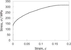
The stress-strain relationship inputted into CPFE simulation for the material properties of the outer edge.
Simulation results are shown in Fig. 13. The results indicate aggregated grains by removing parts of the outer edge. Figure 13(a) and (b) represents stress and strain distributions along the tensile direction, respectively. Some strain concentration is confirmed in the vicinity of GB in Fig. 13(b) due to the difference of crystallographic orientations. Relatively large deformation is observed in grains on the upper part of the model. Local inhomogeneous deformation affected by grain microstructures is well reproduced. A magnitude of stress amplitude at the stress concentration points is not consistent with the strength of common aluminum alloys. This is the reason a large element size was unitized and that the material work-hardening behavior was different from a practical alloy due to insufficient material parameters. Since measurement of inner plastic strain is available in the SRCT by means of tracking markers8), the optimization of material parameters is probably possible by comparing experimental and simulated strains. Therefore, although further optimized calculation had not been performed in this study, complex local heterogeneous deformation in the interior of grain microstructure can be reproduced exhaustively by an image-based simulation model. The construction of an the image-based simulation model of grain microstructure with fine morphology from three-dimensional volume image obtained by high-resolution SRCT helps us to understand the deformation mechanism in a complex microstructure, furthermore, it also helps with the development of more realistic CPFEM by comparing experimental and simulated results.

Demonstration of CPFE simulation using image-based grain-aggregate model; (a) stress distribution along tensile direction and (b) strain distribution along tensile direction.
In this study, the method to build an image-based model from high-resolution X-ray CT image has been proposed for CPFE analysis. Polycrystalline microstructures were investigated in Al-4mass%Cu alloy by X-ray tomography in a synchrotron radiation facility, SPring-8. An image-based model of aggregated grains was reproduced by the proposed method, and the model was analyzed by using classical CPFE analysis. Local deformation analysis of grain microstructures with considering actual grain shapes is possible, and it is suggested that the deformation mechanism would become clear by using the image-based CPFE with further work.
The SPring-8 experiments in this study were carried out as subject numbers of 2012B1013, 2013A1181 and 2013B1027. This work was supported by JSPS KAKENHI Grant Number 24226015 and 26420723. Authors thank The Light Metal Educational Foundation for supporting.