Effect of Particle Shape on the Stereological Bias of the Degree of Liberation of Biphase Particle Systems
2017 Volume 58 Issue 2 Pages 280-286
Details
2017 Volume 58 Issue 2 Pages 280-286
It is well known that in sectional measurements of polished ore samples, the degree of liberation is overestimated by stereological bias. The stereological bias is affected by particle shape, but the effect of particle shape on the stereological bias has not been studied systematically. In this study, particles of various shapes were modeled using a geodesic grid, and the internal structures of the particles were randomly designed. The stereological bias of liberation was assessed quantitatively by comparing the computed sectional information and the original three-dimensional information. The following results were obtained: 1) the effect of aspect ratio on the stereological bias is less than 12% when comparing cases with α ranging from 1.0 to 2.0; 2) the effect of particle surface roughness on the stereological bias is smaller than 7.6% when comparing cases with surface roughness (the quotient of the surface area of the volume equivalent ellipsoid and the surface area of a particle) ranging from 0.833 to 0.996. It was also confirmed that the previously proposed stereological correction method is applicable to irregularly shaped particles because the estimation error of the degree of liberation dramatically dropped from 56.4%–64.4% without any correction to 1.16%–3.41% using the proposed method.
One of the primary purposes of comminution in mineral processing is to achieve valuable mineral liberation at the coarsest particle size possible. This makes it possible to save energy by reducing fine powder production and reducing the cost and effort in the separation process. It is also important to accurately assess the degree of liberation of the comminuted products to feedback correct information and to develop a mineral processing strategy.
In general, to assess the degree of liberation, comminuted materials are hardened with resin and cut, and the polished section is analyzed using an optical microscope or a dedicated analyzer, such as the mineral liberation analyzer1). This two-dimensional (2D) sectional analysis overestimates the degree of liberation, which is called the “stereological bias.” In principle, the stereological bias is unavoidable because in the cutting process, locked particles may become free but free particles cannot become locked2).
The stereological bias is influenced by the internal particle structure. The stereological bias is large in simply locking biphase particles and negligibly small in particles with complex internal structures such as intergrowth3–5). Several studies have been conducted on the stereological bias using spherical particles5–7) and simple regular shaped particles8,9). Because the majority of particles handled in the mining and recycling industries do not have spherical or regular shapes, it is beneficial to study the effect of particle shape on the stereological bias. Remarkable approaches in modeling random particle shape include using Poisson polyhedra10) and PARGEN program wherein the particles are generated through a process that resembles nucleation and growth11). In this study, we propose a new method to model random irregular particle shape with a given value of the aspect ratio and the surface roughness.
A stereological correction method using an integral transformation with the kernel function, which is applicable to irregularly shaped particles, has been proposed12–14). In general, these studies successfully predict the effect of the stereological bias on the liberation distribution of well-examined samples; however, a further systematic investigation is required to confirm their versatility.
Computational simulation is an effective tool in the systematic analysis of the stereological bias because it can accurately and rapidly simulate various patterns of the internal particle structure. To date, methods to model particles with agglomerates of cubic elements with various grain types12) and with spherical particles hollowed out from a Boolean based biphase structure15) have been proposed. We have developed a unique numerical approach wherein the stereological bias of degree of liberation was quantitatively assessed by comparing the three-dimensional (3D) particle internal structures with 2D sectional structures16), a correlation between the 2D texture characteristics and the 3D liberation state was determined5), a stereological correction method was established in which particle sectional textures are assessed, and the 3D liberation state was estimated only from the 2D measureable parameters using a preliminary computed correlation between 2D texture characteristics and 3D liberation state17). Since our numerical simulation has been conducted on spherical binary particle systems, its applicability to more realistic-shaped particle systems needs to be investigated.
In this study, we conducted a series of simulations of the stereological bias of the liberation assessment of particles with various shapes. The goal of this study is to evaluate the effect of particle's aspect ratio and surface roughness on the stereological bias of degree of liberation and to assess the applicability of the proposed stereological correction method to irregularly-shaped biphase particle systems.
Particle shape is quantified using several indices. In this study, we used two indices: aspect ratio ($\alpha$), which represents the general shape of a particle and the surface roughness ($\rho$). $\alpha$ and $\rho$ are defined as follows:
| \[\alpha = \frac{a}{c},\] | (1) |
| \[\rho = \frac{A_c}{A},\] | (2) |
The irregularly shaped particles were modeled using a “geodesic grid,” which is a method to subdivide a sphere using polyhedrons. First, a regular icosahedron inscribed in a sphere was computed (Fig. 1(a)), which is called the first generation. Second, midpoints of all sides were projected on the sphere and new faces were created (Fig. 1(b)), which is called the second generation. This process was continued until the necessary resolution was obtained. The third generation model was used to model particles in this study. Note that a third generation particle has 162 nodes and 320 faces. This procedure was applied to ellipsoids with several values of aspect ratios. Because the aspect ratios of particles produced by brittle fracture take wide range of values but the average is generally less than 2.018,19), we investigated particle models with $\alpha \le 2.0$ in this study.
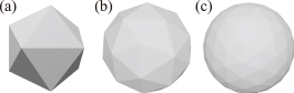
Particles modeled using a geodesic grid: (a) the first generation, (b) the second generation, and (c) the third generation.
Then, the position of each node was dispersed toward the direction from the center of mass of the particle to the node with the following value:
| \[{\rm Dispersion} = \frac{a\varepsilon \gamma}{2},\] | (3) |
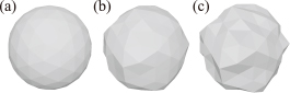
Geodesic grid particles with node dispersions with (a) $\gamma$ = 0.0 (no dispersion), (b) $\gamma$ = 0.5, and (c) $\gamma$ = 1.0.
Particles composed of two phases, phases A and B, were modeled as follows. Figure 3 shows the modeling method schematically.
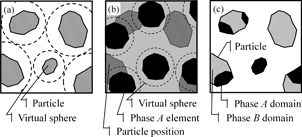
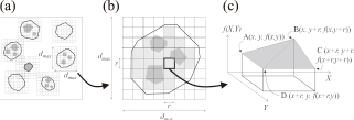
Conceptual diagrams of the particle structure setting procedure: (a) randomly generated virtual spheres are packed into a cuboid and are replaced by irregularly shaped particles at the centers of the spheres with random orientation, (b) irregularly shaped phase A elements are generated in random positions in the same manner but independently of the particles, (c) the overlapping domain between the particles and the phase A elements is set as the phase A domain in the particle, while the rest of the particle is set as the phase B domain.
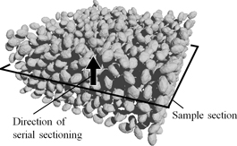
Serial cross-sectional calculation over a particle assembly.
This process is similar to that of Gay6) in the sense that the particles are hollowed from biphase materials; however, it is unique in the modeling of randomly packed particle structures using DEM and irregularly shaped particles. DEM is effective in providing randomly sectioned particles by a single sample sectioning.
Note that various types of 3D biphase structure model has been proposed: the Boolean model6,15), the Poisson mosaic20–22), and the Voronoi tessellation20–22). All of them provide more complex structure than the abovementioned method. Considering the goal of this study of investigating the effect of the particle shape on the stereological bias and on the stereological correction method described below, the abovementioned 3D structure plays a sufficient role.
The sectional information of the biphase particle assembly was calculated using the Monte Carlo method with solid angle calculations, as discussed later. Because the sectional information calculated from different sections varies, this variation should be taken into account along with the stereological bias when comparing sectional information with 3D original information. To avoid the effect of dispersion of each section and investigate the influence of only the stereological bias, multiple sectional information sets should be calculated and statistically processed. With a greater number of calculated sections, the influence of dispersion of each section will lessen; however, this requires more calculation time. In this study, we calculated 20 sections per sample.
2.2 Liberation assessment 2.2.1 Volume and area estimation via the Monte Carlo method with solid angle calculationsThe Monte Carlo method was applied to estimate the volume (or area) of the particles and phase A domains. A number of plots were set at random positions in a volume (or area) including the particles and the phase domain (or their section) and volume (or area), and the volume (or area) of the particles was estimated from the ratio of the numbers of plots inside or outside of the particles and the volume (or area) of the domain. The solid angle calculation described later was used to judge whether the plot was inside or outside the particles. It is possible to estimate the volume (or area) of irregularly shaped particles using the Monte Carlo method; however, its accuracy depends on the number of plots. The effect of the number of plots on the estimation accuracy of the Monte Carlo method was investigated using the error rate (Ev) as follows:
| \[E_v = \frac{100 |V_{geo} - V_{mont}|}{V_{geo}},\] | (4) |
Figure 5(a) and 5(b) plot Ev versus the number of Monte Carlo plots when a sphere and a circle are inscribed in a cube and a square, respectively. The number of plots was increased from 50 in steps of 100, and the average values and standard derivations of every 100 cases are shown as plots and error bars, respectively, in Fig. 5. The error rate decreases with the increasing number of plots in both cases. We applied 80,000 plots in the 3D calculation and 20,000 plots in the 2D calculation as a standard number of plots, in terms of adequately under-run error rate, 0.5% Ev. In the 3D calculation, 80,000 plots were used in the cube circumscribed to a virtual sphere of each particle. In the 2D calculation, the sectional area of the particle varies according to the position of the section. Using the radius of the sectional circle of the virtual sphere ($r_1$) and the radius of the virtual sphere ($r_2$), $20,000 * (r_1/r_2)^2$ plots were used in a square circumscribed to the sectional circle.
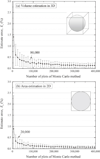
Effect of the number of plots for (a) the volume and (b) area estimations using the Monte Carlo method on the estimation error, Ev. The plots and error bars show the averages and the standard deviations, respectively.
To judge whether the Monte Carlo plots were inside or outside the particles, the solid angle ($\varOmega$) of the particle surface was calculated as follows:
| \[\Omega = \int_S \frac{{\bf t} \cdot {\bf n}}{t^2} dS = \left\{ \begin{array}{@{}ll@{}} 0 & ({\rm when\ the\ plot\ is\ outside}\ S) \\ 4\pi & ({\rm when\ the\ plot\ is\ inside}\ S) \end{array} \right.,\] | (5) |
In 2D, total sectional areas of particles ($A_P$), phases A domain ($A_A$), phase B domain ($A_B$), apparently liberated phase A domain ($A_A^{lib}$), and apparently liberated phase B domain ($A_B^{lib}$) in an arbitrary sample section were calculated through the process in subsection 2.2.1.
In 3D, similarly to 2D, total volumes of particles ($V_P$), phase A domain ($V_A$), phase B domain ($V_B$), liberated phase A domain ($V_A^{lib}$), and liberated phase B domain ($V_B^{lib}$) in the cuboid were calculated.
In statistical processing of the 2D and 3D information, the area fraction and volume fraction of the phase A domain ($F_a$, $F_v$), the degrees of the apparent liberation in 2D for phases A and B ($L_A^{2D}$, $L_B^{2D}$), and the liberation in 3D for phases A and B ($L_A^{3D}$, $L_B^{3D}$) were calculated as follows.
| \[F_a = \frac{1}{\rm n} \sum_1^n \frac{A_A}{A_P}\] | (6) |
| \[F_v = \frac{V_A}{V_P}\] | (7) |
| \[L_A^{2D} = \frac{1}{\rm n} \sum_1^n \frac{A_A^{lib}}{A_A}\] | (8) |
| \[L_B^{2D} = \frac{1}{\rm n} \sum_1^n \frac{A_B^{lib}}{A_B}\] | (9) |
| \[L_A^{3D} = \frac{V_A^{lib}}{V_A}\] | (10) |
| \[L_B^{3D} = \frac{V_B^{lib}}{V_B}\] | (11) |
In addition, to assess the stereological bias quantitatively, the difference between the degrees of apparent liberation in 2D and those of liberation in 3D for phases A and B ($L_A^{2D-3D}$, $L_B^{2D-3D}$) and the ratio of the overestimated liberation in 2D for phases A and B ($\sigma_A$, $\sigma_B$) were calculated as follows.
| \[L_A^{2D-3D} = L_A^{2D} - L_A^{3D}\] | (12) |
| \[L_B^{2D-3D} = L_B^{2D} - L_B^{3D}\] | (13) |
| \[\sigma_A = \frac{L_A^{2D-3D}}{L_A^{2D}}\] | (14) |
| \[\sigma_B = \frac{L_B^{2D-3D}}{L_B^{2D}}\] | (15) |
A stereological correction method using the fractal dimension ($\delta$) of the virtual surface area of the image intensity5,23) has been developed17). A brief introduction to the method is given below.
First, δ is obtained as follows:
Estimation of image surface area A(r). (a) dmax sized square mesh are superimposed on particle cross-sections. (b) The square is divided into r mesh, where the mesh elements enveloped into particle cross-sections are shaded. (c) Surface area of the image intensity of mesh elements in particle cross-sections at a resolution of r is calculated5,23).
| \[\log A(r) = (2 - \delta) \log r + C,\] | (16) |
Second, the ratio of the overestimated liberation in 2D ($\sigma$) is estimated using Fig. 7 (after17) $\sigma_B$ is shown here), which is an isogram of $\sigma$ obtained from the encompassing calculation of 2,764 types of biphase spherical particles17). $\sigma$ value estimated from Fig. 7 is defined as $\sigma'$ for convenience.
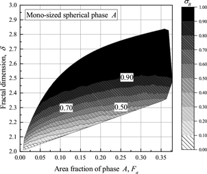
Isogram of the ratio of the overestimated liberation in 2D for phase B ($\sigma_B$) versus the fractal dimension ($\delta$) and area fraction of the phase A ($F_a$) obtained from a series of simulations with spherical particles of various sizes and volume fractions of spherical phase A elements17).
Finally, the degree of liberation in 3D is estimated using the following equation with $\sigma'$ and $L^{2D}$.
| \[L^{3D'} = (1 - \sigma')L^{2D},\] | (17) |
A total of 12 types of particles were designed, where the particles were modeled using the third generation of a geodesic grid with three values of aspect ratio ($\alpha$), 1.0, 1.5, and 2.0, and four values of dispersion ($\gamma$), 0.0, 0.5, 1.0, and 1.5. Figure 8 shows the surface roughness ($\rho$) and $\alpha$ of the 12 types of particles together with their parameters. The ratio of lengths of the long axis (a) and short axis (c) is determined by $\alpha$, and length of the middle axis (b) is designated as the geometric mean of a and c, $\surd (ac)$. In the case of $\alpha = 2.0$, a is equal to the diameter of the vertical sphere ($d_A$), and b and c are calculated from the abovementioned ratio. In cases with $\alpha$ = 1.0 and 1.5, a, b, and c are determined from the particle volume of the corresponding $\alpha = 2.0$ case satisfying the abovementioned length ratio.
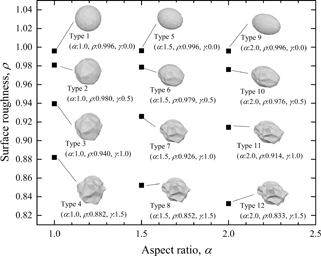
Twelve types of particles with various aspect ratio ($\alpha$) and particle surface roughness ($\rho$). $\gamma$ is a dispersion parameter for particle surface roughness modeling (eq. (3)).
The phase A element is modeled using a first-generation sphere-based geodesic grid with $\gamma = 0.0$. As shown in Table 1, two types of sizes and distributions of phase A elements are computed.
| Type | Phase A element size (dA) | Volume fraction* | Number of phase A elements |
|---|---|---|---|
| Small phase A element | 1.20 | 0.152 | 1,290 |
| Large phase A element | 1.90 | 0.151 | 325 |
* Volume fraction here represents that of the initial condition (Fig. 3(b)).
Figure 9 shows part of a section of a simulation sample with type 11 particles ($\alpha$ = 2.0, $\rho$ = 0.914) and small phase A elements as an example. Middling particles and apparently liberated particles with phases A and B were successfully computed in a random manner.
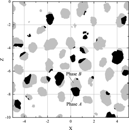
Partial image of a section of a simulation sample with type 11 particles ($\alpha$ = 2.0, $S_c$ = 0.914) and small phase A elements. The black and gray regions denote the phase A and B domains, respectively.
Figure 10 compares $L_A^{2D-3D}$ and $L_B^{2D-3D}$ for various values of $\gamma$ and $\alpha$. Regardless of the $\gamma$ values, the $L_A^{2D-3D}$ of large phase A elements becomes larger than that of small phase A elements, in agreement with the previous study5). The $L_A^{2D-3D}$ of large phase A elements is dispersed with $\gamma$ values. This is because the number of phase A elements is small in this case (Table 1) and the liberation state variations from each particle shape has a considerable effect on the cumulative $L_A^{2D-3D}$ values. The $L_A^{2D-3D}$ of particles with $\alpha$ = 2.0 becomes 0.014 (12%) larger than that of particles with $\alpha$ = 1.0 in this case. Meanwhile, the $L_A^{2D-3D}$ of the small phase A element case slightly decreases with increasing $\alpha$. The $L_A^{2D-3D}$ of particles with $\alpha$ = 2.0 becomes 0.0056 (7.5%) smaller than that of particles with $\alpha$ = 1.0 in this case.
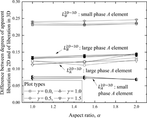
Effect of the aspect ratio ($\alpha$) on differences between the degrees of apparent liberation in 2D and 3D for phases A ($L_A^{2D-3D}$) and B ($L_B^{2D-3D}$).
On the other hand, the $L_B^{2D-3D}$ of large phase A elements becomes smaller than that of small phase A elements regardless of $\gamma$ values, also in agreement with the previous study5). The $L_B^{2D-3D}$s of both the large and small phase A element cases slightly increase with increasing $\alpha$. The $L_B^{2D-3D}$ of particles with $\alpha$ = 2.0 becomes 0.0030 (1.3%) larger than that of particles with $\alpha$ = 1.0 when the phase A element is small. Similarly, it becomes 0.0099 (7.4%) larger when the phase A element is large.
To summarize the above results, the effect of the aspect ratio on the stereological bias is less than 12% when comparing cases with $\alpha$ ranging from 1.0 to 2.0.
4.3 Effect of surface roughnessFigure 11 compares $L_A^{2D-3D}$ and $L_B^{2D-3D}$ for various values of $\alpha$ and surface roughness ($\rho$). In Fig. 11, $L_A^{2D-3D}$ of large phase A elements is dispersed with $\gamma$ values for the same reason discussed for Fig. 10. First, let us compare cases with $\rho$ = 0.996 (for $\gamma$ = 0.0) and $\rho$ = 0.833–0.882 (for $\gamma$ = 1.5). When the phase A element is large, $L_A^{2D-3D}$ with $\alpha$ = 1.5 increases but those with $\alpha$ = 1.0 and 2.0 decrease with decreasing $\rho$, and $L_A^{2D-3D}$ decreases 0.0099 (7.6%) on average. When the phase A element is small, $L_A^{2D-3D}$ with $\alpha$ = 2.0 increases slightly but those with $\alpha$ = 1.0 and 1.5 decrease slightly with decreasing $\rho$, and $L_A^{2D-3D}$ decreases 0.0023 (3.2%) on average.
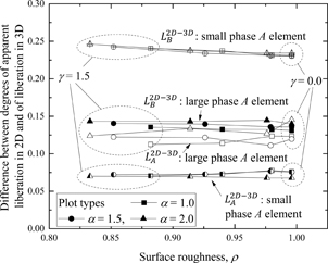
Effect of the surface roughness ($\rho$) on differences between the degrees of apparent liberation in 2D and 3D (a) for phase A ($L_A^{2D-3D}$) and (b) for phase B ($L_B^{2D-3D}$).
On the other hand, in Fig. 11, $L_B^{2D-3D}$s of both large and small phase A element cases increase slightly with decreasing $\rho$. The $L_B^{2D-3D}$ with $\rho$ = 0.833–0.882 becomes 0.0042 (3.1%) larger than that with $\rho$ = 0.996 when the phase A element is large. Similarly, it becomes 0.011 (4.8%) larger when the phase A element is small.
In summary, the effect of the particle surface roughness on the stereological bias of the liberation is smaller than 7.6% when comparing cases with $\rho$ ranging from 0.833 to 0.996.
4.4 Stereological correctionStereological correction method in subsection 2.3 was applied to the large and small phase A cases (Table 1) with 12 types of particles (Fig. 8). Phase B liberation was assessed here because the isogram of $\sigma_B$ (Fig. 7) was presented in Ref. 17). The computational simulation results show that for small phase A elements, $F_a$ = 0.1514–0.1518 and $\delta$ = 2.217–2.222. Similarly, for large phase A elements, $F_a$ = 0.1516–0.1522 and $\delta$ = 2.217–2.222. Here, the small phase A element case is included in the map in Fig. 7, but large small phase A element case is not included. In a future study, we will enlarge the map area with additional simulation cases, but here just the small phase A element case was validated. The estimation error of the degree of liberation ($E_{lib}$) was compared between cases with and without stereological correction.
| \[E_{lib} = 100\frac{|L_B^{3D} - L_B^{est}|}{L_B^{3D}},\] | (18) |
Figure 12 compares the $E_{lib}$s of 12 types of particles (Fig. 8). The $E_{lib}$s without the stereological correction have values of 56.4–64.4%, while after the proposed correction, they dramatically decrease to 1.16–3.41%. Therefore, the proposed stereological correction method is applicable to irregularly shaped particles, although further validation with various types of particles is required.
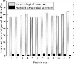
Estimated error of the degree of liberation with and without the proposed stereological correction for 12 types of particles (Fig. 8) with small phase A elements.