Abstract
Morphology and crystallography of second phases, such as precipitates, martensites, inclusions, etc., embedded in a parent phase are discussed. The contribution of elastic strain energy is considered to find the most favorable shape of a second phase for given eigenstrains and elastic constants. Analyses based on the idea of invariant plane and invariant line deformations are conducted to discuss crystallography and energetics of second phases. Simple criteria are proposed to explain orientation relationship between the second phase and the parent phase as well as epitaxial relationship for substrate/thin film systems. Two types of stress effects are discussed; one on the morphology of the second phase and the other on variant selection.
This Paper was Originally Published in Japanese in Materia Japan 56 (2017) 331–337. Since the maximum page allowance of this overview was larger than that for the Japanese version in Materia Japan, more detailed descriptions and explanations were possible. Accordingly, Chapters 2, 4 and 5 were made longer and Keywords and References were revised. Tables 1 and 2, and Figs. 6 and 8 as well as some equations were newly added.
1. Introduction
Crystalline second phases embedded in a solid parent phase show various types of morphology. In addition, they often exhibit certain crystallographic orientation relationships with the parent-phase crystal. In this overview, factors controlling the morphological and crystallographic aspects of second phases, such as precipitates, martensites, inclusions, etc., will be discussed by reviewing previous studies including those by the present author and his colleagues. In particular, the contribution of elastic strain energy will be considered in detail to find the favorable shape of a second phase. Eshelby's ellipsoidal inclusion theory of elasticity1,2) will be used for the analysis. In addition, we will also deal with the crystallography and epitaxy between a substrate crystal and a thin film crystal deposited onto the substrate.
For a martensitic transformation to produce plate-shaped martensite, experimental results of habit plane orientation and orientation relationship between the martensite and the parent phase are often compared with calculated ones from the so-called phenomenological crystallographic theories of martensitic transformations.3–6) The basic concept behind the phenomenological theories is that the habit plane, i.e., a planar interface between the parent phase and the martensite, be an invariant plane. Since Patel and Cohen published a classic paper,7) effects of applied stress on martensitic transformations have been discussed through the interaction between the applied stress and the total shape deformation (invariant plane deformation) of the martensites, despite the fact that martensites are not necessarily plate-like in shape. In this overview, the stress effects on the phase transformation will also be discussed.
For the above purposes, we will adopt both the finite-deformation (FD) approach and the infinitesimal-deformation (ID) approach. The former will be used when crystallography and orientation relationship are to be analyzed and the latter will be used when elasticity is applied to evaluate the elastic states and energetics associated with the formation of second phases and thin films.
2. Energetics and Thermodynamics
When a second phase of volume Ω appears in a parent phase as a result of a phase transformation, e. g., precipitation, martensitic transformation, etc., the change in the total energy ΔGT is generally expressed as
| \[
\varDelta G_{\rm T} = \varDelta G_{\rm C} + E_{\rm el} + E_{\rm interface},
\] | (1) |
where
ΔGC (< 0) is the chemical driving force,
Eel (> 0) the elastic strain energy due to transformation strains or lattice misfit strains,
Einterface (> 0) the interface energy due to the difference in atomic arrangements and/or atomic species across the interface between the parent phase and the second phase. The transformation is considered to proceed when
ΔGT becomes negative.
The second and the third terms of the right-hand side of eq. (1) constitute the changes in the mechanical energy, or the Helmholtz energy,8) ΔF if the phase transformation takes place under an isothermal condition.
| \[
\varDelta F = E_{\rm el} + E_{\rm interface}.
\] | (2) |
In this overview, the phase transformation under the isothermal condition will be considered and a second phase will often be called a particle. Aside from kinetic aspects, the stable or most favorable shape of the particle is thermodynamically determined so as to minimize
ΔF in eq. (2). Since
Eel is proportional to the third power and
Einterface is proportional to the second power of the particle size, the former becomes more important as the particle size becomes larger.
When stress is applied during the phase transformation, thermodynamic discussion based on Gibbs energy8) must be conducted by taking into account additional stress-dependent energy terms. This case will be treated later in Chapter 5.
With thermodynamics as a fundamental tool, the most favorable morphology and crystallography of second-phase particles will be discussed by applying the free energy minimization criterion. In the following, transformation strains and lattice misfit strains will be collectively called eigenstrains.8)
3. Shape Stability and Crystallography of Second Phases
Let us first consider the case when applied stress is absent and, therefore, the minimization of the Helmholtz energy ΔF (eq. (2)) determines the shape of a second-phase particle. As mentioned above, when particles are small, the interface energy Einterface is a dominant factor of determining the particle shape. It goes without saying that a sphere is most favorable when isotropic interface energy is assumed. When interface energy is anisotropic, it is well known that the equilibrium particle shape can be obtained through the so-called Wulff construction.9) What happens then when the elastic strain energy Eel becomes the dominant factor of determining the particle shape? In most of this overview, we will neglect the interface energy term Einterface in eq. (2) and only the contribution of Eel will be taken into account to avoid unnecessary complication. More involved analyses including the term Einterface will be introduced later by referring to our previous studies.
In what follows, the particle shape is approximated as a spheroid shown in Fig. 1:
| \[
\frac{\xi_{1}^{2}}{a^{2}}
+
\frac{\xi_{2}^{2}}{a^{2}}
+
\frac{\xi_{3}^{2}}{(\alpha a)^{2}}
\le
1,
\] | (3) |
where the
$(\xi_{1}, \xi_{2}, \xi_{3})$ orthogonal coordinates are taken parallel to the three principal axes of the spheroid, 2
a and 2
αa are the lengths of the principal axes with
$\alpha\ ( > 0)$ being the aspect ratio. The spheroid represents a plate or a disc when
$\alpha \to 0$, a sphere when
$\alpha = 1$, and a needle or a rod when
$\alpha \to \infty$. The volume
Ω of the spheroid is given by
$\varOmega = 4\pi\alpha a^{3}/3$.
The uniform eigenstrains εij in the particle are described on the $(x_{1}, x_{2}, x_{3})$ orthogonal coordinates fixed to the parent phase as
| \[
\varepsilon_{ij}
=
\left(
\begin{array}{ccc}
\varepsilon & 0 & 0 \\
0 & \varepsilon & 0 \\
0 & 0 & k\varepsilon
\end{array}
\right),
\] | (4) |
where
ε and
k are real quantities. Although eq. (4) represents tetragonal eigenstrains, various types of eigenstrains can be expressed by changing the value of
k. For example, isotropic eigenstrains with
$k = 1$, shear type eigenstrains with
$k = - 2$, uniaxial eigenstrains with
$k \to \pm \infty$, etc. As shown in
Fig. 1, the
ξ3 axis of the spheroid is tilted with respect to the
x3 axis of the parent phase by the angle
θ and the
x2 and
ξ2 axes are set parallel to each other without loss of generality.
We further consider that the elastic constants of the particle $C_{ijkl}^*$ are f $(\ge 0)$ times larger than those of the parent phase $C_{ijkl}$ :
| \[
C_{ijkl}^{*} = fC_{ijkl}.
\] | (5) |
Elastic strain energy Eel was evaluated for particles with various combinations of α, k and f by using Eshelby's ellipsoidal inclusion theory for isotropic elasticity.1,2) If Eel varied with the orientation θ for a given set of α, k and f, the angle θ was chosen so that Eel became minimum, Emin. Figure 2 shows the elastic strain energies of plate, sphere and needle particles for (a) $k = 1$ and (b) $k = - 2$ as a function of the ratio of elastic constants f.10,11) Poisson's ratio ν was assigned to be ν = 1/3 for both parent and second phases. It is well known that when $k = 1$ and $f = 1$, Eel is independent of the shape of the particle.10,11) From Figs. 2 (a) and (b), we can also say that the plate shape has the smallest strain energy and, thus, thermodynamically most stable when the particle is softer than the parent phase ($0 \le f < 1$). However, if the particle is harder than the parent phase, the favorable shape with minimum strain energy varies depending on the values of k and f.

By repeating the above analysis, the most favorable shape (or aspect ratio α) to give the minimum strain energy was obtained for given k and f. The results are shown in Fig. 3.12) It is interesting to find that the plate is always most favorable when the particle is softer than the parent phase ($0 \le f < 1$), and the sphere is most favorable only for harder particles ($f > 1$) with isotropic eigenstrains ($k = 1$).

We have so far discussed the stable shape of a particle by considering the contribution of the elastic strain energy Eel only. In some of our previous studies, we have included the effects of interface energy Einterface as well as elastic anisotropy.13–15) Furthermore, not only coherent particles, elastic states of incoherent particles as a result of plastic accommodation have also been discussed.10,16–18) In particular, it should be pointed out that the elastic strain energy vanishes for a fully accommodated incoherent plate.10,17) This fact will be referred to later in Chapter 4.
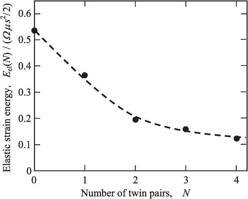
Now, I would like to introduce you to one of my memorable research experiences. Aging of a Cu-1mass%Fe alloy results in coherent precipitation of metastable γ-Fe spherical particles in a Cu matrix.19) Since $k = 1$ and $f > 1$ for this case, the spherical shape is understood to be most favorable even for the contribution of elastic strain energy only (see Fig. 3). When uniaxial stress is applied to this aged alloy, stress-induced fcc (γ) → bcc (α) martensitic transformation occurs in the Fe particles and they become internally twinned α-Fe.19) When I was a graduate student in the mid-1970s, a new ellipsoidal inclusion theory was developed and the evaluation of the elastic states of an inclusion with periodically distributed eigenstrains became possible.20) As an application of this new theory, we tried to calculate the elastic strain energy of an internally twinned α-Fe particle in the Cu matrix. As shown in Fig. 4, the internal twinning was modeled by alternating layers of anti-parallel shears with the shear eigenstrains $\varepsilon_{31} = \varepsilon_{13} = \pm s/2$. Our purpose was to calculate the elastic strain energy Eel(N) of the particle as a function of the number of twin pairs N. For $N = 0$, Eel(0) can be obtained analytically from the original Eshelby theory. However, for $N \ge 1$, even if isotropic and homogeneous elasticity is adopted, numerical calculation on a computer is inevitable. Since no such things as personal computers were available in the mid-1970s, all the numerical calculations were performed at a university computer center with programs edited and stored line by line on punched cards.

After many efforts, Fig. 5 was obtained.19,20) Eel(N) appears to decrease as N increases. This can be understood intuitively: As N increases, the particle shape becomes closer to a sphere (see Fig. 4). In addition, experimental results show that N increases as the particle size increases.19) The increase in N induces the increase in the twin-boundary energy. Therefore, the number of twin pairs in an α-Fe particle is considered to be determined by the balance between the decrease in the elastic strain energy and the increase in the twin-boundary energy.19)
One of the remaining problems of interest is what happens in Fig. 5 as N becomes even larger: Does Eel(N) asymptotically approach a certain value, or does it become zero? What is the physical meaning behind either of the two cases? Different from the mid-1970s, it should be easy to numerically examine this problem now.
4. Crystallography and Energetics of Planar Interfaces
Crystallography of planar interfaces, such as habit planes of second phases and interfaces of substrate/thin film systems, often becomes a topic in both scientific and technological studies. Let us first consider how a certain orientation relationship, if any, is realized between two abutting crystals across a planar interface.
One of the geometrical theories to successfully analyze the interface crystallography is the O-lattice theory developed by Bollmann.21,22) According to the theory, the three dimensional O-lattice formed by two crystal lattices I and II is made of the assembly of O-lattice vectors ${\bf X}^{\rm O}$ defined as
| \[
({\bf I} - {\bf T}^{-1}){\bf X}^{\rm O} = {\bf b}^{\rm L}.
\] | (6) |
Here,
I is the
$3 \times 3$ unit matrix,
T the transformation matrix to change the lattice from Lattice I to Lattice II,
${\bf T}^{-1}$ the inverse matrix of
T, and
${\bf b}^{\rm L}$ an arbitrary translation vector of Lattice I.
It is well known that the degree of geometrical matching between the two lattices becomes higher as the absolute value of the determinant of the matrix ${\bf I} - {\bf T}^{-1}$, $|\det ({\bf I} - {\bf T}^{-1})|$, becomes smaller.23–25) Therefore, the highest degree of matching is realized when $|\det ({\bf I} - {\bf T}^{-1})| = 0$ is satisfied. Mathematically, this means that the rank r of the $3 \times 3$ matrix ${\bf I} - {\bf T}^{-1}$ is either zero, one or two. We are not interested in the case of $r = 0$, since T becomes a unit matrix so that Lattices I and II are identical. On the other hand, when $r = 1$, the matrix T represents the invariant plane deformation and when $r = 2$, it represents the invariant line deformation.26–28)
4.1 Invariant plane deformation and incoherent second phases
As mentioned in Introduction, the phenomenological crystallographic theories of martensitic transformations3–6) are based on the invariant plane deformation. Here, the habit plane is considered to be an invariant plane satisfying no-strain and no-rotation conditions.
Let us further examine the implication of the invariant plane deformation by adopting the ID approach. For this purpose, a martensite plate is described by eq. (3) with $\alpha \to 0$. Although eigenstrains to transform Lattice I to Lattice II are usually expressed on the basis of the $(x_{1}, x_{2}, x_{3})$ parent phase coordinates such as those in eq. (4), they will be expressed here as $\varepsilon_{ij}^{\xi}$ on the basis of the $(\xi_{1}, \xi_{2}, \xi_{3})$ coordinates of the martensite with the $\xi_{3}$ axis perpendicular to the invariant habit plane. From the definition of the invariant plane, all the transformation eigenstrain components in the plane are zero, i.e.
| \[
\varepsilon_{11}^{\xi} = \varepsilon_{22}^{\xi} = \varepsilon_{12}^{\xi} = 0.
\] | (7) |
According to Eshelby's ellipsoidal inclusion theory, elastic strain energy per unit volume
E0 for a plate inclusion is written as
8)
| \[
E_{0} = \left(
\frac{\mu}{1-\nu}
\right)
\{
(\varepsilon_{11}^{\xi})^{2}
+
(\varepsilon_{22}^{\xi})^{2}
+
2\nu (\varepsilon_{11}^{\xi} \varepsilon_{22}^{\xi})
+
2(1 - \nu) (\varepsilon_{12}^{\xi})^{2}
\},
\] | (8) |
where
μ is the shear modulus of the inclusion. Therefore, when eq. (7) holds,
E0 of eq. (8) becomes zero. This is the physical interpretation of the martensite habit plane being an invariant plane. The formation of the invariant plane is energetically most favorable since no elastic strain energy is created upon the martensitic transformation.
29–32) Furthermore, recalling the comments mentioned in Chapter 3, we can say that a plate martensite with an invariant habit plane is regarded as a fully accommodated incoherent second phase from the micromechanics point of view.
4.2 Invariant line deformation and geometrical criteria for interface crystallography
The invariant line deformation criterion28) has been applied to explain various orientation relationships between two crystals. From eq. (8), it is found that the eigenstrain components $\varepsilon_{31}^{\xi}$, $\varepsilon_{32}^{\xi}$ and $\varepsilon_{33}^{\xi}$, if any, create neither stresses nor elastic strain energy. As a result, the stresses in the plate inclusion always satisfy the plane-stress condition of $\sigma_{31}^{\xi} = \sigma_{32}^{\xi} = \sigma _{33}^{\xi} = 0$. This implies that eq. (8) is applicable to the evaluation of the elastic strain energy of a substrate/thin film system with the $\xi_{3}$ axis perpendicular to the interface.
On the $\xi_{1} - \xi_{2}$ interface plane of a plate second phase or of a substrate/thin film interface, one can obtain principal eigenstrains $\varepsilon_{11}^{\xi} = \varepsilon_{1}^{\rm P}$ and $\varepsilon_{22}^{\xi} = \varepsilon_{2}^{\rm P}$ by choosing $\xi_{1}^{\rm P}$ and $\xi_{2}^{\rm P}$ principal axes on which the two-dimensional eigenstrain matrix becomes diagonal. In other words, on the $(\xi_{1}^{\rm P}, \xi_{2}^{\rm P}, \xi_{3})$ coordinates, eq. (8) becomes
| \[
E_{0} = \left(
\frac{\mu}{1-\nu}
\right)
\{
(\varepsilon_{1}^{\rm P})^{2}
+
(\varepsilon_{2}^{\rm P})^{2}
+
2\nu (\varepsilon_{1}^{\rm P} \varepsilon_{2}^{\rm P})
\}.\] | (9) |
Since Poisson's ratio is about one third for many materials, the parameter
M defined as
| \[
M \equiv (\varepsilon_{1}^{\rm P})^{2}
+
(\varepsilon_{2}^{\rm P})^{2}
+
\frac{2}{3}
\varepsilon_{1}^{\rm P}
\varepsilon_{2}^{\rm P}
\] | (10) |
is approximately proportional to the elastic strain energy
E0.
We have evaluated the degree of geometrical matching as well as orientation relationships between two different crystals to from a planar interface. We have found that the following geometrical criteria are very well applicable to explain interface crystallography:27,28)
(i) When an appropriate lattice correspondence to relate two crystal lattices, Lattice I and Lattice II, is chosen, two abutting planes to form a planer interface are related to each other by the chosen lattice correspondence.
(ii) With the above lattice correspondence, FD-based two-dimensional affine transformation A from Lattice I to Lattice II can be described by principal eigenstrains $\varepsilon_{1}^{\rm P}$ and $\varepsilon_{2}^{\rm P}$ on the $(\xi_{1}^{\rm P}, \xi_{2}^{\rm P})$ interface coordinates:27,28,33)
| \[
{\bf A} =
\left(
\begin{array}{cc}
1 + \varepsilon_{1}^{\rm P} & 0 \\
0 & 1 + \varepsilon_{2}^{\rm P}
\end{array}
\right).
\] | (11) |
If these principal strains satisfy
| \[
\varepsilon_{1}^{\rm P}\ \varepsilon_{2}^{\rm P} \le 0,
\] | (12) |
the invariant line exists on the interface.
26–28) and such an interface is most preferred. The orientation relationship between the two crystals is determined in such a manner that an invariant line is formed on the interface. On the other hand, if the principal strains do not satisfy the inequality (12), the orientation relationship is determined so that the two principal-strain directions of both lattices become parallel to each other.
(iii) If multiple candidates for interface orientation still exist even after Criterion (ii) is taken into account, the interface with the smallest M value (eq. (10)) is most preferred.
Figure 6 shows the idea of the invariant line deformation.26) The two-dimensional transformation A in eq. (11) is expressed on the principal $(\xi_{1}^{\rm P}, \xi_{2}^{\rm P})$ coordinates. Suppose the vector ${\bf V}_{\rm I}$ is a special vector whose length remains unchanged by the transformation ${\bf A}$. In general, its direction changes from ${\bf V}_{\rm I}$ to ${\bf V}_{\rm II}$ upon the transformation. From ${\bf V}_{\rm II} = {\bf AV}_{\rm I}$ and $| {\bf V}_{\rm II}| = |{\bf V}_{\rm I}|$, the two vectors and their angle ϕ can be found. As a second step after the application of ${\bf A}$, Lattice II is rotated by ϕ with respect to Lattice I. This rotation matrix ${\bf Q}$ is written as
| \[
{\bf Q} = \left(
\begin{array}{cc}
\cos\phi & - \sin\phi \\
\sin\phi & \cos\phi
\end{array}
\right).
\] | (13) |
The transformation
${\bf A}$ and the rotation
${\bf Q}$ result in the total deformation
${\bf T}$ :
| \[
{\bf T} = {\bf QA}.
\] | (14) |
After the total deformation
${\bf T}$,
${\bf V}_{\rm II}$ coincides with
${\bf V}_{\rm I}$ and the original
${\bf V}_{\rm I}$ direction becomes the invariant line direction
${\bf V}_{\rm inv}$. The necessary condition for the existence of the invariant line is that the two principal eigenstrains be different in sign, i.e., the inequality (12).
26–28)
We have applied the above Criteria (i), (ii) and (iii) to discuss crystallographic features of interfaces between fcc and bcc crystals. Both fcc and bcc sides of the interface are assumed to be made of single crystals and the well-known Bain correspondence34,35) shown in Fig. 7 is adopted as the lattice correspondence in Criterion (i). Hereafter, the subscripts f and b will denote fcc and bcc lattices, respectively.
The mutually Bain-corresponding fcc and bcc planes and directions can be found as follows. The bcc plane corresponding to the fcc $(h,k,l)_{\rm f}$ plane is obtained as33,36)
| \[
(h,k,l)_{f}\ \left(
\begin{array}{@{}ccc@{}}
1/2 & 1/2 & 0 \\
-1/2 & 1/2 & 0 \\
0 & 0 & 1
\end{array}
\right)
\equiv
((h - k)/2,(h + k)/2,l)_{\rm b}.
\] | (15) |
On the other hand, the bcc direction corresponding to the fcc
$[a,b,c]_{f}$ direction becomes
33,36)
| \[
\left(
\begin{array}{ccc}
1 & -1 & 0 \\
1 & 1 & 0 \\
0 & 0 & 1
\end{array}
\right)\
\left[
\begin{array}{c}
a \\
b \\
c
\end{array}
\right]_{\rm f}
\equiv
\left[
\begin{array}{c}
a - b \\
a + b \\
c
\end{array}
\right]_{\rm b}.
\] | (16) |
Criterion (i) says that when the fcc side of the interface plane is
$(h,k,l)_{\rm f}$, the bcc side of the interface plane becomes
$((h - k)/2,(h + k)/2,l)_{\rm b}$. On this interface, two mutually perpendicular vectors,
${\bf x}_{\rm f}$ along the
$\xi_{1}^{\rm P}$ axis and
${\bf y}_{\rm f}$ along the
$\xi_{2}^{\rm P}$ axis, can be found uniquely so that they are related to two mutually perpendicular vectors
${\bf x}_{\rm b}$ and
${\bf y}_{\rm b}$, respectively, by the Bain correspondence of eq. (16).
27,28,33) In other words, these principal direction vectors satisfy
${\bf x}_{\rm f} \bot {\bf y}_{\rm f}$,
${\bf x}_{\rm b} \bot {\bf y}_{\rm b}$,
${\bf x}_{\rm f}//{\bf x}_{\rm b}$ and
${\bf y}_{\rm f}//{\bf y}_{\rm b}$. The Bain-corresponding planes and mutually perpendicular directions constituting the fcc/bcc interface are summarized in
Table 1.
33) From the principal direction vectors, the principal eigenstrains
$\varepsilon_{1}^{\rm P}$ and
$\varepsilon_{2}^{\rm P}$ are obtained as
| \[
\varepsilon_{1}^{\rm P}
=
\frac{|{\bf x}_{\rm b}| a_{\rm b}}{|{\bf x}_{\rm f}| a_{\rm f}}
- 1,
\varepsilon_{2}^{\rm P}
=
\frac{|{\bf y}_{\rm b}|a_{\rm b}}{|{\bf y}_{\rm f}| a_{\rm f}}
- 1,
\] | (17) |
where
$a_{\rm f}$ and
$a_{\rm b}$ are the lattice parameters of fcc and bcc crystals, respectively. From
$\varepsilon_{1}^{\rm P}$ and
$\varepsilon_{2}^{\rm P}$, the angle
ϕ in
Fig. 6 to form an invariant line direction on the interface is calculated as
26–28)
| \[
\cos\phi
=
1
+
\frac{\varepsilon_{1}^{\rm P} \varepsilon_{2}^{\rm P}}{2 + (\varepsilon_{1}^{\rm P} + \varepsilon_{2}^{\rm P})}.
\] | (18) |
To examine the matching of fcc and bcc crystals at a planar interface and to apply the above geometrical criteria, the (112)
f plane of a solid-solution Cu-47 at%Ni single crystal was prepared and used as a substrate. This alloy has almost the same room-temperature lattice parameter as that (extrapolated) of γ-Fe. On the Cu-Ni(112)
f substrate, α-Fe thin film was vacuum deposited and the morphology and crystallography of α-Fe were examined by a transmission electron microscope.
33) From eq. (15), we find that there are two different bcc planes corresponding to {112}
f. They are {123}
b and {012}
b, as listed in
Table 2. For the respective correspondences, the principal directions
${\bf x}_{\rm f}$ and
${\bf y}_{\rm f}$ on the fcc side of the interface and
${\bf x}_{\rm b}$ and
${\bf y}_{\rm b}$ on the bcc side of the interface can be found from
Table 1 and are shown in
Table 2. From these directions, the values of the principal eigenstrains
$\varepsilon_{1}^{\rm P}$ and
$\varepsilon_{2}^{\rm P}$ are obtained from eq. (17) with lattice parameter values
af = 0.356 nm and
ab = 0.286 nm.
33) As seen in
Table 2, between the (112)
f ⇔ (123)
b and (112)
f ⇔ (012)
b correspondences, only the former satisfies the inequality (12). Therefore, according to Criterion (ii), the Cu-Ni(112)
f//α-Fe(123)
b interface is preferred over the Cu-Ni(112)
f//α-Fe(012)
b interface. The experimental results show that this was indeed the case for the Cu-Ni/α-Fe system.
33) Moreover, not only the interface planes, but also the observed orientation relationship on the Cu-Ni(112)
f//α-Fe(123)
b interface could be explained satisfactorily with Criterion (ii): The calculated angle
ϕ from eq. (18) perfectly explained the observed epitaxial relationship between Cu-Ni and α-Fe crystals.
33)

Another example is again based on our experiments: The (001)b, (101)b and (111)b planes of α-Fe single crystals were used as substrates and Cu thin film was deposited onto them.37) It was found that the Cu(001)f plane was formed on α-Fe(001)b, the Cu(111)f plane on α-Fe(101)b, and the Cu(021)f plane on α-Fe(111)b. All these bcc/fcc interfaces satisfy the Bain correspondence of eq. (15). Therefore, Criterion (i) holds for all the cases. Although the α-Fe(001)b//Cu(001)f interface does not satisfy the invariant line condition, the epitaxy could be understood by the M parameter in Criterion (iii). Using both Criteria (ii) and (iii), the observed α-Fe(101)b//Cu(111)f interface together with its epitaxial relationship could be explained reasonably. Furthermore, the α-Fe(111)b//Cu(021)f epitaxy was in agreement with the invariant line criterion (ii).37)
I would like to conclude this chapter by saying that such simple geometrical criteria as above are in fact widely applicable to explain observed orientation relationships and epitaxial relationships between two crystals, in particular for metal/metal systems.38)
5. Stress Effects
5.1 Shape stability
If stress σij is applied during a phase transformation, in addition to the Helmholtz energy ΔF of eq. (2), other new terms must be considered for the discussion of thermodynamic stability.8,39,40)
| \[
\varDelta G \equiv \varDelta F + G_{\rm I} + G_{\rm I}^{\rm m}
=
E_{\rm el} + G_{\rm I} + G_{\rm I}^{\rm m},
\] | (19) |
where
ΔG is the change in the mechanical Gibbs energy caused by the appearance of the second phase
Ω under
σij,
$G_{\rm I}$ the interaction energy between
σij and
Ω due to the eigenstrains
εij in
Ω, and
$G_{\rm I}^{\rm m}$ the interaction energy between
σij and
Ω due to the difference in the elastic constants between
Ω and the parent phase. The interface energy term
Einterface in eq. (2) was again neglected in the third term of eq. (19) for simplicity. For given
k (eq. (4)) and
f (eq. (5)), the stable shape
α (eq. (3)) to minimize
ΔG can be obtained as a function of the applied stress.
Pineau studied this stress effect on the shape-dependent stability of the second-phase particle for k = 1 and $0 \le f < \infty$ based on eq. (19).39) The case for a uniaxial applied stress $\sigma_{33}^{\xi} = \sigma$ parallel to the ξ3 axis of the spheroid was considered. However, he took into account only three representative shapes; plate, sphere and needle. As a refinement of Pineau`s work, we have considered the stable particle shape with an arbitrary value of α.40) The results are summarized in Fig. 8.40) The energetically most favorable spheroidal shape for a given combination of σ and f is shown. As can be seen, there are wide regions, overlooked by Pineau, where either oblate or prolate spheroids are most stable. Furthermore, we find that a sphere is stable only on three boundary lines.

Later, the analysis on the shape stability under stress has been extended to treat the case for many similar particles distributed in a parent phase.41) Nevertheless, our studies40,41) treated the shape stability under stress for only one case of fixed eigenstrains k = 1. Different assignment of k would result in a completely different favorable shape diagram. Furthermore, eigenstrains themselves may change upon the application of stress if the microstructure of a second phase is stress dependent. The readers should refer to the overview42) and the lecture note43) by Mori on this point.
5.2 Variant selection
For the case of homogeneous elastic constants of f = 1, i.e., when the elastic constants of the second phase are the same as those of the parent phase, the term $G_{\rm I}^{\rm m}$ vanishes39,40) and eq. (19) is simplified to be
| \[
\varDelta G = E_{\rm el} + G_{\rm I},\ {\rm for}\ f = 1.
\] | (20) |
In fact, if
f is close to unity, the term
$G_{\rm I}^{\rm m}$ is known to be small compared with the term
$G_{\rm I}$.
44) Therefore, unless the elastic constants of the second phase is much larger or much smaller than those of the parent phase, eq. (20) is a physically meaningful approximation.
When the eigenstrains εij do not depend on the applied stress σij, Eel in eq. (20) is independent of σij. Then, the minimization of ΔG is realized when $G_{\rm I}$ becomes minimum. The explicit expression of $G_{\rm I}$ is written as8,40,44,45)
| \[
G_{\rm I}
=
- \varOmega \sum_{i=1}^{3} \sum_{j=1}^{3} \sigma_{ij}\
\varepsilon_{ij},\
{\rm for}\ f = 1.
\] | (21) |
In many second–phase particles, certain number of crystallographically equivalent variants exist. For example, the lattice change associated with fcc (γ) to bcc (α) martensitic transformation in iron alloys is known to occur by the Bain deformation (see Fig. 7)
| \[
{\bf B} =
\left(
\begin{array}{ccc}
\sqrt{2} a_{\rm b}/ a_{\rm f} & 0 & 0 \\
0 & \sqrt{2} a_{\rm b}/ a_{\rm f} & 0 \\
0 & 0 & a_{\rm b}/ a_{\rm f}
\end{array}
\right),
\] | (22) |
for the FD approach and by the Bain strain
| \[
\begin{split}
\varepsilon_{ij}^{\rm B}
&=
\left(
\begin{array}{@{}ccc@{}}
(\sqrt{2} a_{\rm b}/ a_{\rm f}) - 1 & 0 & 0 \\
0 & (\sqrt{2} a_{\rm b}/ a_{\rm f}) - 1 & 0 \\
0 & 0 & (a_{\rm b}/a_{\rm f}) - 1
\end{array}
\right)\\
&=
\left(
\begin{array}{@{}ccc@{}}
\varepsilon_{11}^{\rm B} & 0 & 0 \\
0 & \varepsilon_{22}^{\rm B} & 0 \\
0 & 0 & \varepsilon_{33}^{\rm B}
\end{array}
\right),
\end{split}
\] | (23) |
for the ID approach where the inequalities
| \[
\varepsilon_{11}^{\rm B} = \varepsilon_{22}^{\rm B} > 0,\ \varepsilon_{33}^{\rm B} < 0
\] | (24) |
hold for iron alloys. From (24), we know that the fcc lattice is contracted along the
$x_{3}// [001]_{\rm f}$ axis and extended along the
$x_{1}// [100]_{\rm f}$ and
$x_{2}// [010]_{\rm f}$ axes to transform into the bcc lattice. Since the fcc parent phase has cubic symmetry, there are two other crystallographically equivalent Bain strains; one with the contraction axis
$[100]_{\rm f}$ and the other with the contraction axis
$[010]_{\rm f}$.
The three Bain strain variants are equivalent in a sense that they are equally operative upon the $\gamma \to \alpha$ martensitic transformation taking place by simple cooling. However, when stress σij is applied to induce the transformation, the three variants are no more equivalent and the one with the smallest $G_{\rm I}^{\rm B}/\varOmega$ value defined as
| \[
G_{\rm I}^{\rm B}/\varOmega \equiv
-
\sum_{i=1}^{3}
\sum_{j=1}^{3}
\sigma_{ij}\ \varepsilon_{ij}^{\rm B}.
\] | (25) |
would be formed preferentially over the other two Bain variants. This is the phenomenon of the so-called variant selection: preferential formation of specific variants among crystallographically equivalent ones.
During my graduate student days, I was engaged in research on the stress-induced $\gamma \to \alpha$ martensitic transformation in iron alloys under the guidance of my respected advisors, Professors Tsutomu Mori and Akikazu Sato. We have used single crystals of fcc alloys; Fe-23Ni-5Cr,46,47) Cu-1Fe19) and Fe-30Ni-0.5C.48) Either uniaxial tension or uniaxial compression was applied to these single crystals and preferentially formed stress-induced bcc martensite variants were examined. The phenomenon of the variant selection in stress-induced martensitic transformations was already well known even at that time. However, most experimental studies were conducted using polycrystalline specimens. Therefore, we decided to examine the stress effects under simplified situations using single crystals.
Just before our studies, stress-induced formation of α lath martensites in Fe-18Ni-14Cr single crystals was examined by Higo et al.49) The martensitic transformations in all the above four alloys19,46–49) are the same in terms of the lattice change from fcc (γ) to bcc (α). However, the shapes of the martensites are quite different; a needle for Fe-23Ni-5Cr, a sphere for Cu-1Fe, a plate for Fe-30Ni-0.5C and a lath for Fe-18Ni-14Cr. Nevertheless, It was surprising to find that when a uniaxial stress was applied along a prescribed crystallographic direction of the parent γ phase, preferentially formed nearly Kurdjumov-Sachs (KS)50) α variants were essentially the same regardless of the shape of the stress-induced martensites.
When I was a graduate student, and maybe even now, stress effects were discussed mainly through the interaction between the stress and the total shape deformation involved in the martensitic transformation; the well known hypothesis by Patel and Cohen.7) According to the phenomenological crystallographic theories mentioned in Introduction and Chapter 4,3–6) the deformation ${\bf T}$ for the total shape change is composed of lattice-change deformation (the Bain deformation for $\gamma \to \alpha$) ${\bf B}$, lattice-invariant deformation (either by slip or by twinning) ${\bf P}$ and rigid-body rotation ${\bf R}$. Using the FD approach, we can write
| \[
{\bf T} = {\bf R\, P\, B}.
\] | (26) |
Among the above four iron base alloys, ${\bf B}$ is common. However, ${\bf T}$ is completely different since the martensite shape is quite different. Therefore, the fact that the preferentially formed KS variants were the same indicates that stress effects on the martensitic transformation appear on the Bain deformation ${\bf B}$ but not on ${\bf T}$, in contradiction to the Patel-Cohen hypothesis. In other words, our experimental results indicate that the preferentially formed variants are those which minimize $G_{\rm I}^{\rm B}/\varOmega$ in eq. (25). A similar conclusion can be derived if we consider further decomposition of the Bain deformation ${\bf B}$ into two $\{111\}_{\rm f} \langle 211 \rangle_{\rm f}$ shear systems.51)
During the transformation, the deformation ${\bf B}$ must occur in early stages of the transformation. This is because there is no reason for ${\bf P}$ and ${\bf R}$ to occur unless ${\bf B}$ occurs. Therefore, our conclusion can also be said that the stress effects are significant in the early stages of the martensitic transformation.
The stress effects on the variant selection have been studied by many investigators. There is enough evidence that the stress effects appear in the early stages of martensitic transformation and precipitation.52–58) Furthermore, the interaction energy GI of eq. (21) has been applied successfully to explain the variant selection for preferential precipitation on dislocations by regarding σij as dislocation stress fields and εij as the transformation strains of the precipitate.59–61)
6. Concluding Remarks
In this overview, factors controlling the morphology and crystallography of second phases embedded in a crystalline parent phase are surveyed. The contribution of elastic strain energy is discussed using the ellipsoidal inclusion theory by Eshelby. Simple criteria based on the invariant plane and invariant line deformation conditions are proposed to discuss the energetic interpretation of the martensite habit plane, and orientation relationship between two different crystals that meet at a planar interface. In addition, interaction between eigenstrains and applied stress is discussed for the shape stability of a second phase under stress as well as for the stress-induced variant selection in martensitic transformations.
Nearly forty years have passed since I started my academic career as a postdoc at Northwestern University. Since then, methods and techniques for experiment, analysis and calculation have been advanced significantly. Current researchers are good at handling highly sophisticated experimental, analytical and computational facilities and present various new findings which could not have been obtained forty years ago. However, it appears that many fundamental knowledge and understanding developed several decades ago are still valid and useful even now. In this sense, I hope this overview, containing results of rather old-fashioned studies, is still of some help to current researchers.
Acknowledgments
I would like to express my sincere appreciation to my advisors, colleagues and former students for their excellent guidance and cooperation in conducting many experimental and theoretical studies. Thanks are also due to the Japan Institute of Metals and Materials for giving me the opportunity to publish this overview.
REFERENCES
- 1) J.D. Eshelby: Proc. R. Soc. Lond. A Math. Phys. Sci. 241 (1957) 376–396.
- 2) J.D. Eshelby: Prog. Solid. Mech. 2 (1961) 89–140.
- 3) M.S. Wechsler, D.S. Lieberman and T.A. Read: Trans. Metall. AIME 197 (1953) 1503–1515.
- 4) J.S. Bowles and J.K. Mackenzie: Acta Metall. 2 (1954) 129–137.
- 5) J.K. Mackenzie and J.S. Bowles: Acta Metall. 2 (1954) 138–147.
- 6) J.S. Bowles and J.K. Mackenzie: Acta Metall. 2 (1954) 224–234.
- 7) J.R. Patel and M. Cohen: Acta Metall. 1 (1953) 531–538.
- 8) T. Mura: Micromechanics of Defects in Solids, 2nd, revised edition, (Murtinus Nijhoff Publishers, Dordrecht, 1987).
- 9) T. L. Einstein: Handbook of Crystal Growth, IA, Fundamentals, 2nd edition, ed. by T. Nishinaga, (Elsevier, Amsterdam, 2015) Chapter 5.
- 10) M. Kato, T. Fujii and S. Onaka: Mater. Sci. Eng. A 211 (1996) 95–103.
- 11) M. Kato, T. Fujii and S. Onaka: Mater. Trans., JIM 37 (1996) 314–318.
- 12) T. Fujii, S. Onaka and M. Kato: Scr. Metall. 34 (1996) 1529–1535.
- 13) S. Onaka, N. Kobayashi, T. Fujii and M. Kato: Intermetallics 10 (2002) 343–346.
- 14) N. Kobayashi, S. Onaka, T. Fujii and M. Kato: Mater. Sci. Eng. A 392 (2005) 248–253.
- 15) C. Kanno, K. Aoyagi, T. Fujii and M. Kato: Philos. Mag. Lett. 90 (2010) 589–598.
- 16) T. Mori, M. Okabe and T. Mura: Acta Metall. 28 (1980) 319–325.
- 17) M. Kato and T. Fujii: Acta Metall. Mater. 42 (1994) 2929–2936.
- 18) M. Kato, T. Fujii and S. Onaka: Acta Mater. 44 (1996) 1263–1269.
- 19) M. Kato, R. Monzen and T. Mori: Acta Metall. 26 (1978) 605–613.
- 20) T. Mura, T. Mori and M. Kato: J. Mech. Phys. Solids 24 (1976) 305–318.
- 21) W. Bollmann: Philos. Mag. 16 (1967) 363–381.
- 22) W. Bollmann: Philos. Mag. 16 (1967) 383–399.
- 23) J. W. Christian and A. G. Crocker: Dislocations in Solids, Vol. 3, ed. by F. R. N. Nabarro, (North Holland, Amsterdam, 1980) 165–249.
- 24) R.C. Ecob and B. Ralph: Proc. Natl. Acad. Sci. USA 77 (1980) 1749–1753.
- 25) S. Hashimoto: Materia Japan 22 (1983) 151–157.
- 26) U. Dahmen: Acta Metall. 30 (1982) 63–73.
- 27) M. Kato: Tetsu-to-Hagané 78 (1992) 209–214.
- 28) M. Kato: Mater. Trans., JIM 33 (1992) 89–96.
- 29) M. Kato, T. Miyazaki and Y. Sunaga: Scr. Metall. 11 (1977) 915–919.
- 30) K. Mukherjee and M. Kato: J. de Phys., Colloq. C4 43 (1982) C4-297–C4-302.
- 31) M. Kato and M. Shibata-Yanagisawa: J. Mater. Sci. 25 (1990) 194–202.
- 32) M. Shibata-Yanagisawa and M. Kato: Mater. Trans., JIM 31 (1990) 18–24.
- 33) M. Kato and T. Mishima: Philos. Mag. A 56 (1987) 725–733.
- 34) E.C. Bain: Trans. Metall. AIME 70 (1924) 25–46.
- 35) J.S. Bowles and C.M. Wayman: Metall. Trans. 3 (1972) 1113–1121.
- 36) M. Kato, S. Fukase, A. Sato and T. Mori: Acta Metall. 34 (1986) 1179–1188.
- 37) M. Kato, T. Kubo and T. Mori: Acta Metall. 36 (1988) 2071–2081.
- 38) K.H. Westmacott, S. Hinderberger and U. Dahmen: Philos. Mag. A 81 (2001) 1547–1578.
- 39) A. Pineau: Acta Metall. 24 (1976) 559–564.
- 40) S. Onaka, Y. Suzuki, T. Fujii and M. Kato: Scr. Metall. 38 (1998) 783–788.
- 41) S. Onaka, T. Fujii, Y. Suzuki and M. Kato: Mater. Sci. Eng. A 285 (2000) 246–252.
- 42) T. Mori: Mater. Trans. 44 (2003) 901–906.
- 43) T. Mori: Materia Japan 55 (2016) 528–531.
- 44) M. Kato and H.-r. Pak: Phys. Status Solidi 130 (1985) 421–430 (b).
- 45) M. Kato and H.-r. Pak: Phys. Status Solidi 123 (1984) 415–424 (b).
- 46) M. Kato and T. Mori: Acta Metall. 24 (1976) 853–860.
- 47) M. Kato and T. Mori: Acta Metall. 25 (1977) 951–956.
- 48) A. Sato, M. Kato, Y. Sunaga, T. Miyazaki and T. Mori: Acta Metall. 28 (1980) 367–376.
- 49) Y. Higo, F. Lecroisey and T. Mori: Acta Metall. 22 (1974) 313–323.
- 50) G. Kurdjumov and G. Sachs: Z. Phys. 64 (1930) 325–343.
- 51) A.J. Bogers and W.G. Burgers: Acta Metall. 12 (1964) 255–261.
- 52) T. Eto, A. Sato and T. Mori: Acta Metall. 26 (1978) 499–508.
- 53) Y. Tanaka, A. Sato and T. Mori: Acta Metall. 26 (1978) 529–540.
- 54) A. Sato and M. Kato: Tetsu-to-Hagané 69 (1983) 1531–1539.
- 55) M. Shibata, M. Kato, H. Seto, T. Noma, M. Yoshimura and S. Somiya: J. Mater. Sci. 22 (1987) 1432–1436.
- 56) A. Sato, S. Katsuta and M. Kato: Acta Metall. 36 (1988) 633–640.
- 57) M. Kato, T. Fujii, Y. Hoshino and T. Mori: J. Jpn. Inst. Metals 56 (1992) 865–872.
- 58) R. Monzen and M. Kato: ISIJ Int. 33 (1993) 898–902.
- 59) M. Kato, S. Onaka and T. Fujii: Sci. Technol. Adv. Mater. 2 (2001) 375–380.
- 60) T. Fujii, H. Ogawa, S. Onaka and M. Kato: J. Jpn. Inst. Metals 66 (2002) 989–996.
- 61) T. Fujii, S. Onaka and M. Kato: Materia Japan 43 (2004) 925–930.