Quantification of Localized Water Image in Under-Film Corroded Steel with High Spatial Resolution, High Time Resolution, and Wide View by Neutron Radiography

Abstract

Information on the existence of localized water at corrosion locations is indispensable for precisely understanding the corrosion mechanism in steel. Small amounts of localized water in under-film corrosion have not yet been measured quantitatively.

Although we have demonstrated that neutron radiography, which has high sensitivity to the presence of hydrogen, is suitable method for detecting of water in the under-film corrosion of painted steel by utilizing the RIKEN Accelerator-driven Neutron Source (RANS), the spatial and time resolutions were insufficient to investigate under-film corrosion in detail. We then performed an imaging experiment on localized water in steel corrosion with higher space and time resolutions using the high-intensity neutron source at J-PARC. We obtained data with a spatial resolution of 0.6 mm, a time resolution of 15 s in a viewing area of 100 × 100 mm². On the basis of the results for the quantitative imaging of localized water in corrosion, we have established a method suitable for directly imaging water in steel corrosion that employs neutrons.

Fig. 4 Changes in water distributions with time.

1. Introduction

Steel is the most widely used material in infrastructure, transportation, and manufacturing. As the corrosion of steel has a huge cost to society,¹⁾ steels are painted with films as a low-cost measure against corrosion. However, so-called “under-film corrosion” inevitably occurs in outdoor environments because of exposure to cycles of wet and dry conditions. Since water is a factor determining wet corrosion,²⁾ it is important to quantify water existing in under-film corrosion to investigate the corrosion of painted steel.

There are various methods obtaining information of the corrosion environment in terms of the existence of water, such as an index called time of wetness,³⁾ which is determined by climate information, including temperature and humidity, as well as atmospheric corrosion monitoring^4,5) and quartz crystal microbalance^6,7) methods. However, they provide macroscopic data and no direct information on the water. In particular, small amounts of localized water in corrosion, considered to be related to the progression of corrosion, are extremely difficult to be measure by these methods.

To directly detect water in under-film corrosion, we have started to apply neutron radiography, which is sensitive to light elements such as hydrogen, using the RIKEN Accelerator-driven Neutron Source (RANS).⁸⁾ We have recently observed the time dependence of the water distribution in under-film corrosion of painted steel.⁹⁾ In the study, by comparing neutron radiographic images of dry and wet samples, a technique for the quantitative observation of only the water distribution was proposed, then the amounts of water in corrosion blisters of normal steel and anti-corrosion alloy steel were measured. Although we succeeded in measuring amount of water in the blister with entire area of 1000 mm², we could not use explicitly a term of spatial resolution due to such large area, because of the insufficient neutron intensity at RANS. Then, we have performed an experiment to prove that a neutron imaging method can quantify the water movement both in a localized space and in a short time period, at Japan Proton Accelerator Research Complex (J-PARC), which provides a high-intensity and highly parallel neutron beam. Our aim was to achieve a spatial resolution of (less than) 1 mm with area of 1 mm², one tenth of typical blister width of 10 mm, and a time resolution of less than 30 s, one-tenth of that for the RANS experiment. These resolutions in both spatial and time could bring the first quantitative measure for the study on under film corrosion of steel. This experiment allowed us to simultaneously view most of the area of interest of a large corrosion blister. As an extension of time dependent water distribution, we derived an image, showing the average water content ratio, which was used to visualize the distribution of water accumulation in the corrosion blister.

In this paper, the neutron radiography for obtaining for time dependence of water distribution in under-film corrosion with high spatial and time resolutions is described. Also, a visualization method is focused on to demonstrate the high precision of the image data.

2. Experiment

2.1 Samples

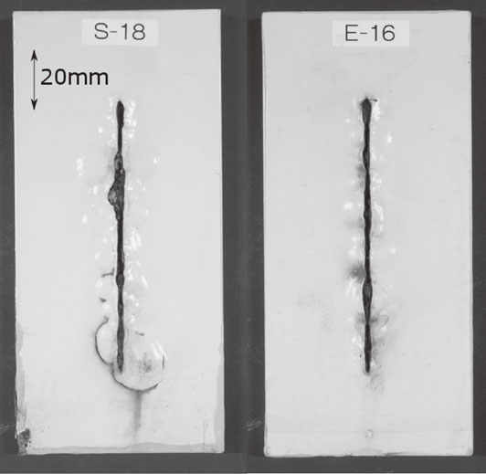
The two plate samples of normal steel (SM400)¹⁰⁾ and alloy steel (0.8Cu–0.4Ni–0.05Ti) used in this study were identical to those in our previous studies.^8,9) Both samples were 6 mm thick, 70 mm wide, and 140 mm high. They were coated with 0.24-mm-thick epoxy-modified paint and scratched by a sharp knife. Then the plates were subjected to a cyclic corrosion test for 6 months.¹¹⁾ Photographs of the samples are shown in Fig. 1. The scratch is at the center of the sample with a blister around the scratch. The boundary between the blister and non-blister regions is visible and it is defined as the edge of the blister.

Fig. 1

Photographs of samples. Left: normal sample, right: alloy sample.

2.2 Neutron beam at sample position

The neutron beamline BL-10^12,13) at the J-PARC Materials and Life Experimental Facility¹⁴⁾ was used in this experiment. Neutrons were produced by injecting 3 GeV protons into a mercury target via nuclear spallation reactions with a repetition rate of 25 Hz. The neutrons were slowed to the energy range of cold neutrons in a moderator and extracted at locations from the viewed surface of the moderator to the sample position. As the number of produced neutrons was proportional to the number of protons, the flux intensity at the sample was normalized by the number of protons, which was monitored during the experiment. In this study, J-PARC was operated at a proton beam power of 200 kW. The flux of neutrons, whose energy was less than 0.4 eV, was estimated to be 1 × 10⁷ n/s/cm² at the sample position. The angle divergence of the neutron beam was 1/140 rad. The beam size at the sample position was 100 × 100 mm². For comparison, in the previous study⁹⁾ at RANS, the neutron beam intensity, angle divergence, and beam size were about 10⁴ n/s/cm², 1/36 rad, and 150 × 150 mm² at the sample position, respectively.

2.3 Sample setup and detector system

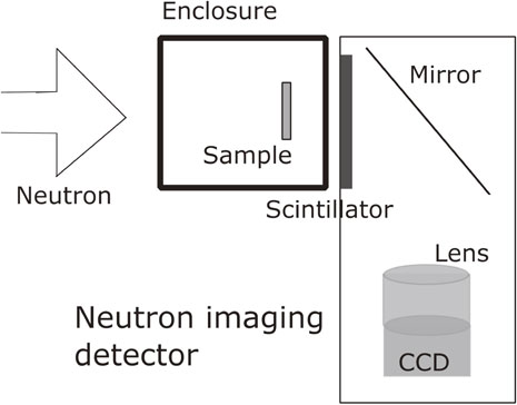
The sample was placed in a hermetic box to avoid the effect of environmental humidity, which was set at a distance of 14 m from the moderator. The experimental setup is shown in Fig. 2. A two-dimensional neutron detector was located downstream of the hermetic box. The distance between the sample and the scintillator was determined to be 78 mm so that the detector was as close as possible to the sample.

Fig. 2

Experimental setup for sample and neutron imaging detector.

The neutron detector shown in Fig. 2 was composed of a 400-µm-thick ⁶LiF(Ag)/ZnS scintillator,⁹⁾ a mirror and lenses (light focus optics), and a charge coupled device (CCD) camera operated at 0°C to reduce the thermal noise in the images.¹⁵⁾ The sensitive area on the scintillator was 146 mm in height and 106 mm in width. The pixel size of the camera was 41 µm × 41 µm and the number of pixels was 2672 × 4008. The visible light from the scintillator, whose intensity was proportional to the number of neutrons, was detected by the camera.

2.4 Measurement procedure

Before the exposure to neutrons, the samples were soaked in distilled water for 2 h, which is sufficient time for the saturation of the amount of water. After each sample was removed from the water, the water on the surface was wiped off. Then the sample was mounted in the box. Neutron exposure was started after 30 min after removing the sample from water.

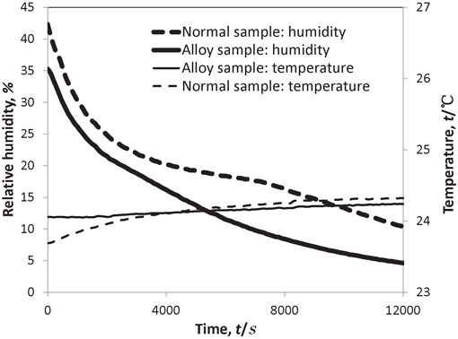
The air in the box was ventilated during neutron exposure by flowing 2000 cm³/min of dry air through the box. The measured humidity and temperature in the box are shown in Fig. 3. The variation of the temperature in the box was within 0.5°C. The humidity in the box was 35 relative humidity (RH) % at the beginning and decreased in an exponential-like curve.

Fig. 3

Humidity and temperature during measurement.

We first determined the optimum exposure time by observing the responses of the detector with different neutron exposure times without the sample in the box. According to the results, an exposure time of 12 s did not saturate the CCD camera. This 12 s is much shorter than exposure time of 5 to 10 min in the RANS experiments.⁷⁾ There was a 3 s interval between two consecutive images. While taking the neutron images, the number of protons was counted to monitor the neutron beam flux. The image data were saved along with the start time of the exposure and the number of protons.

3. Data Analysis

3.1 Principle

We first describe how water was identified using neutrons. The water-containing samples (wet samples) were dried in the box during neutron exposure. The normal and alloy samples at times of 14000 and 12000 s after the start of the exposure, respectively, are referred to as the dry samples, because of very small change in the contrast of the images. By comparing images of the wet and dry samples, the distribution of the water was obtained. In the dry samples there were two possible sources of hydrogen in steel corrosion: FeOOH and the painted film materials. Images of these two hydrogens sources were canceled out by subtracting the dry image from the wet image, enabling us to derive the water distribution.

Here we denotes neutron absorption length of water, $L_{H_{2}O}$, as the distance which the incident neutron flux decreases 1/e in the water and thickness of water, $t_{H_{2}O}$, as water thickness along neutron beam direction, which equals to sample thickness direction. Neutron absorption length of dry sample, L_d, and thickness of dry sample, t_d, are defined for the dry sample as well. Incident neutron flux for the dry and wet samples are denoted as $I_{d}^{0}$ and $I_{d + H_{2}O}^{0}$, respectively. The neutron fluxes transmitted through the dry and wet samples are I_d and $I_{d + H_{2}O}$, which are expressed to be   

\begin{equation} I_{d} = I_{d}^{0}e^{-\frac{t_{d}}{L_{d}}} \end{equation} (1)

and   

\begin{equation} I_{d + H_{2}O} = I_{d + H_{2}O}^{0}e^{-\frac{t_{d}}{L_{d}} - \frac{t_{H_{2}O}}{L_{H_{2}O}}}. \end{equation} (2)

Terms regarding to the dry sample, t_d and L_d are cancelled out by dividing eq. (2) by eq. (1), and then the relation between these parameters⁷⁾ is given be the following equation.   

\begin{equation} t_{H_{2}O} = L_{H_{2}O}\cdot Log\left(\frac{I_{d}}{I_{d + H_{2}O}}\cdot\frac{I_{d + H_{2}O}^{0}}{I_{d}^{0}}\right) \end{equation} (3)

The first term in the logarithm in eq. (3) was calculated from the pixel-by-pixel ratio. The second term in the logarithm is the ratio of the incident flux, which should be the same value for all pixels because the spatial profile of the neutron beam was expected to be stable over time. This term was derived from the neutron ratio at area where neutrons enter into the detector directly without passing through the sample.

The value of $L_{H_{2}O}$ was estimated to be 6.7 mm using a radiation tracking-code as described in the previous paper.⁹⁾ Since the density of water is 1 mg/mm³, the amount of water in a specific area can be computed by multiplying the thickness of water by the area.

3.2 Optimal pixel size for imaging

Owing to the angle divergence of the neutron beam of BL-10,^12,13) the unsharpness of the neutron image was 0.6 mm, which was obtained as the product of 78 mm (the distance between the sample and the scintillator) and 1/140 rad (the angle divergence), which limited the spatial resolution of the measured water distributions. According to the sampling thereom,¹⁶⁾ a suitable pixel size for the imaging detector is half of the spatial resolution. As a result, the optimized pixel size was chosen to be 0.2 × 0.2 mm², which was achieved by merging 5 × 5 CCD pixels into one pixel.

3.3 Experimental errors

The neutron flux at J-PARC BL-10 beamline slightly changes with time owing to the fluctuation of the proton beam current. If the integrated neutron flux during the 12 s exposure time varies, the correlation coefficient between the brightness on the camera and the number of detected neutrons will change, since the sensor on the camera has a maximum non linearity of 1%,¹⁷⁾ and then all the variables in logarithmic terms of eq. (1) may have an error. Therefore, only images for which number of protons was within 0.5% of the average value were used for the data analysis to eliminate these fluctuations and thus reduce the error.

The ratio ${\frac{I_{d}}{I_{d}^{0}}}$ in eq. (1) is the neutron transmission ratio of the dry sample. Although its actual value should be constant, a measurement value may vary statistically. To reduce the statistical fluctuation, an image averaged over ten images at the end of the exposure was used as the dry image instead of a single image to obtain I_d and $I_{d}^{0}$.

4. Results and Discussion

4.1 Water distribution

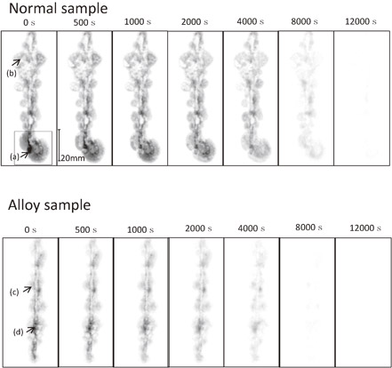
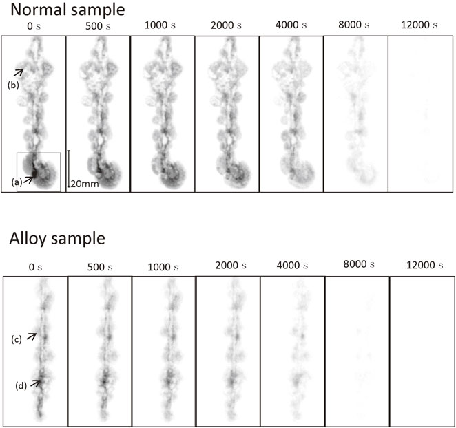
Figure 4 shows images of the water distributions in both samples at times of 0, 500, 1000, 2000, 4000, 8000, and 12000 s after the start of exposure. The contrast in the images indicates the amount of water, dark parts have more water than light parts. The same scale of contrast was applied to the normal and alloy samples. The water distribution at the start of the exposure has a one-to-one correspondence to the blister region shown in Fig. 1, where the outline of the distribution indicates the boundary between the blister and non-blister regions. Figure 4 was obtained by simultaneous imaging with the wide view area covering most of the blister region.

Fig. 4

Changes in water distributions with time.

It was observed that the amount of water in both samples decreased with time. Water still existed in the normal sample at 8000 s but had almost completely disappeared at 12000 s. However, water remained in the alloy sample up to 4000 s and almost completely disappeared at 8000 s.

These water distribution images were taken every 15 s during the experiment. The numbers of images used for the analysis of the normal and alloy samples were 805 and 713, respectively.

For comparison, Fig. 5 shows the water distributions of the same samples obtained at RANS⁷⁾ with the same neutron detector and the same analysis method as used in this paper. The localized water distribution is much clearer in Fig. 4 than in Fig. 5.

Fig. 5

Changes in water distributions with time observed at RANS.

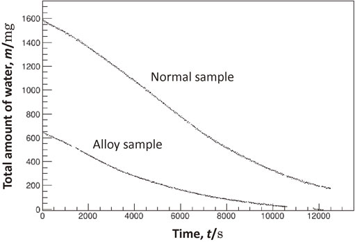
Regarding the total amount of water in the corrosion, the time dependences of the total amount of water in the blister region are shown in Fig. 6. The total amount of water in each sample decreased gradually, decreasing by half at elapsed times of 3000 and 6000 s (T_1/2) for the alloy sample and normal sample, respectively. This result confirms the behavior observed in the previous study at RANS.⁹⁾

Fig. 6

Time dependences of total amount of water per unit area.

4.2 Rapid decreasing in amount of water in localized areas

There are some areas where the water disappears in a short time. The four points with arrows, (a)–(d), in Fig. 4 were chosen to investigate the time dependence of the amount of water amount in localized areas. Sudden changes were observed at the points (a) and (c) indicating a rapid decrease in the amount of water. To show these changes in detail, Fig. 7 shows the time dependences of the amount of water at points (a)–(d) in both samples. The amount of water at point (b) decreases exponentially from 0 to 12000 s. In contrast, at point (a), it remains almost constant until 500 s and then decreases from 0.14 to 0.07 mg/mm² in 30 s, which is equivalent to T_1/2 of 30 s. This suggests the movement of water caused this rapid decrease instead of water evaporation for which T_1/2 was 6000 s. Note that similar rapid decreases were observed at three other measurement points and that a time-resolution of 15 is sufficiently high to observe water movement.

Fig. 7

Typical examples of time dependences of amount of water in 0.2 × 0.2 mm² areas. (a)–(d) indicate the positions in Fig. 4.

For the alloy sample, the amount of water at point (c) decreases suddenly at 1000 s but the decrease is only 0.02 mg/mm², and smaller than that at point (a). The amount of water at the point (d) does not show a rapid decrease but the decrease is gradual.

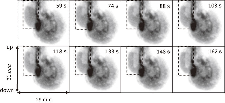
To observe the spatial distributions of water in the areas where rapid decreases occurred, Fig. 8 shows enlarged images of the area of interest, which is surrounded by a 29 × 21 mm solid square in Fig. 4, and includes point (a). Figure 8 shows eight consecutive images taken at times from 59 to 162 s with approximately 15 s intervals. The vertical direction in the images is pointed by “up” and “down” in the figure.

Fig. 8

Enlargement of area surrounded by the solid square in Fig. 4 including point (a) and changes with time from 59 to 162 s.

Focusing on the area enclosed by the doted rectangle in Fig. 8, it is observed that the water moved downward from 59 s to 74 s, remained at the same height from 88 to 133 s, moved downward again from 133 to 148 s, and then remained stationary until 162 s. It is noteworthy that the amount of water decreased nonuniformly in space.

4.3 Observation of increasing in amount of water

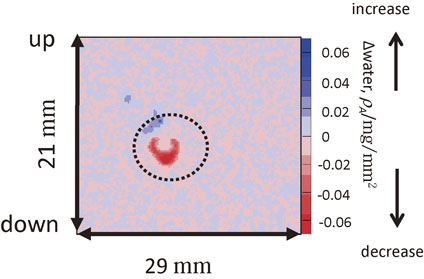
Figure 9 shows three consecutive enlarged images of the same area as in Fig. 8 taken from 473 to 502 s. In the center of the doted circle as in Fig. 9, an area with a low amount of water expanded with time. To observe this area in detail, a distribution of the change in the amount of water increase/decrease was derived by subtracting the image at 502 s from that at 473 s, as shown in Fig. 10. The doted circle is at the same location as in Fig. 9. A red area, where the amount of water decreased, is located in the circle, and blue areas, where the amount of water increased, are located at the top and above of the circle. It is notable that these movements occurred within 30 s.

Fig. 9

Enlargement of area surrounded by the solid square in Fig. 4, including point (a) and changes with time from 473 to 502 s.

Fig. 10

Distribution of change in amount water of water calculated by subtracting image at 502 s from that at 473 s.

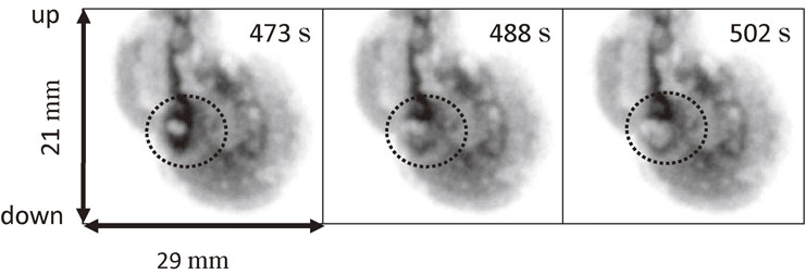
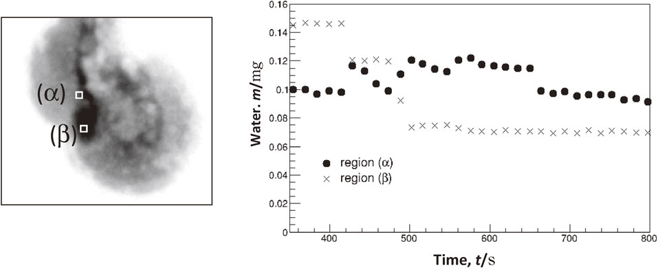
Figure 11 shows the time dependences of the amount of water in squares (α) and (β) near point (a), whose areas are 2 mm × 2 mm. The amount of water in (α) increases from 410 to 420 s, decreases to 480 s, and then increases to 520 s. In (β), it decreases from 410 to 420 s, remains constant until 480 s and then decreases rapidly to 500 s.

Fig. 11

Time dependence of amount of water in specific regions. The left figure shows specific regions of 2 mm × 2 mm and the right figure shows the time dependence in each region.

These increases and decreases are larger than the detection limit, which is discussed in the next section. The rapid increases and decreases in Fig. 11 are 300 times faster than the decrease in the total shown in Fig. 6, and are considered to be due to water movement rather than evaporation.

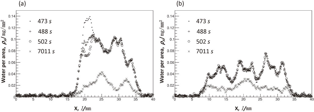
4.4 Profiles of resolved images of water

Horizontal cutaways views, along lines including points (a) and (b) in Fig. 4 showing the amount of water at the different time are given in Figs. 12(a) and (b), respectively. The region from X = 0 to 15 mm in Fig. 12(a) is a flat part without a corrosion blister as shown in Fig. 1. This region has less variation in the amount of water than the region from X = 15 to 37 mm, which corresponds to the blister. It is estimated that the water detection limit is about 0.002 mg/mm² by observing the fluctuation in the flat region. In Fig. 12, the water distribution has some peaks, and the sharpness of the peaks indicates a spatial resolution of 0.6 mm. This resolution corresponds to the value derived in section 3.2 from the divergence of the neutron angle.

Fig. 12

Cutaway views along horizontal lines including points (a) and (b) in Fig. 4 at 473, 488, and 502 s, during which point (a) has a rapidly decreasing amount of water (see Fig. 7), and 7011 s.

In Fig. 12(a), in the localized region from 18 to 22 mm, including point (a), the amount of water decreases by 0.6 mg/mm² within 30 s. In other regions, however, it remains almost constant.

The water is distributed from X = 15 to 36 mm in Fig. 12(a) and from 7 to 35 mm in Fig. 12(b). The widths of the distributions in both (a) and (b) did not change up to 7000 s. This suggests that water can remain at the boundary between the blister and non-blister regions for a long time. Then, we attempted to obtain an enhance image of water accumulation throughout the entire blister with high spatial resolution.

4.5 Formulation of water accumulation

The accumulation of water in a specific area due to the progression of wet corrosion is strongly correlated with the product of the amount of water and the wetness duration.^18–22) We define water accumulation (WA) as the integral of the amount of water with respect to time without the effect of the thickness of the blister. WA is expressed by the following equation:   

\begin{equation} \mathrm{WA}(\boldsymbol{{p}}) = \frac{1}{T}\int_{0}^{T}\frac{w(t,\boldsymbol{{p}})}{w(0,\boldsymbol{{p}})}dt, \end{equation} (4)

where $w(t,\boldsymbol{{p}})$ is the amount of water in a specific area p at a given time t, and T is the period of averaging, which is 12000 s in this study. $w(0,\boldsymbol{{p}})$ denotes the maximum amount of water held by the corrosion layer in a specific area.

WA should take values from 0 to 1 as a dimensionless quantity. If WA is 1, the amount of water remains stable. If WA is near 0, the water disappears soon after the beginning of measurement. Moreover, a high rate of water loss in the blister zone results in a low WA, and vice versa. The values of WA are 0.26, 0.54, 0.31, and 0.47 at points (a), (b), (c), and (d), respectively, in Fig. 4. It is anticipated that the amount of water at point (a) decreased rapidly very early in the measurement as shown in Fig. 6.

4.6 Visualization of water accumulation (WA)

The frequency distributions of WA are shown in Fig. 13. The WA of the normal sample is distributed with higher values than that of the alloy sample. The mean value and standard deviation of the alloy sample are 0.38 and 0.085, whereas those of the normal sample are 0.53 and 0.11, respectively. This observation indicates that the normal sample can hold water for a longer time than the alloy sample. This result is in agreement with the data of the total amount of water in the blister zone in our previous study,⁹⁾ where water in the normal sample remains longer than that in the alloy.

Fig. 13

Frequency distributions of WA.

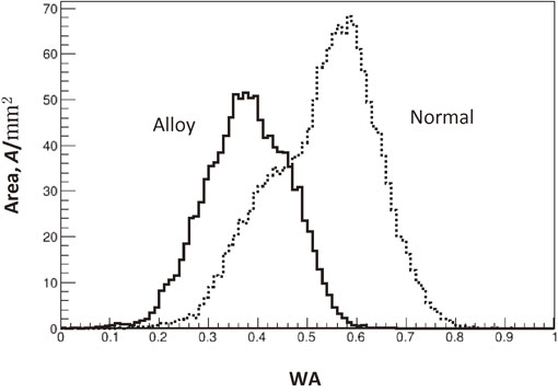
Figure 14 shows the two-dimensional spatial distributions of WA. X and Y describe the position in the unit of mm. The color indicates the WA, where red indicates a high WA and blue indicates a low WA. White areas indicate the non-blister regions, where there is less water than the detection limit, which match the non-blister regions shown in Fig. 1. Number of areas with high WA exists along the edge of the blister region in the normal sample. A similar tendency was observed in the alloy sample, although the values of WA were about half of those for the normal sample and the number of areas with a high WA was small. In addition to the high-WA areas at the edge of the blister regions, there are high-WA areas inside the blister regions in the normal sample. This WA distribution indicates that water remains for a long time along the edge. This is consistent with the observation of no significant change in the width of the water distribution after prolonged time drying as discussed in section 4-4.

Fig. 14

Two-dimensional spatial distributions of WA. Ratio of the length scales in the X to that in Y directions is set to 3:5 for both distributions. Solid lines indicate the positions of the profiles in Fig. 9. Dashed lines indicate locations of the scratch.

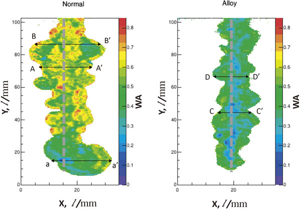
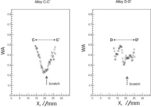
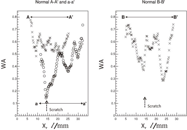
Figures 15 and 16 show profiles of the spatial distributions of WA along the solid lines in Fig. 14. The profile along A–A′ in Fig. 15 shows that WA rapidly decreases from 0.78 to 0.5 within a horizontal distance of approximately 3 mm from X = 7 mm to X = 10 mm. WA in the center of profile A–A′ fluctuates between 0.53 and 0.66 and then increases to 0.65 at the right edge. The large dip at X = 15 mm in the profile along a–a′ corresponds to the scratch. There are two large and steep dips in the profile along B–B′. In contrast to the normal sample, WA for the alloy along profile C–C′ in Fig. 16 is smaller than that for the normal sample. The dip in profile C–C′ corresponds to the scratch of the film, which is shown in Fig. 1, and is neither as deep nor as steep as that for the normal sample. There is a dip with a depth of 0.3 in profile D–D′.

Fig. 15

WA profiles of the normal sample. The positions of lines A–A′, a–a′, and B–B′ are indicated in Fig. 14. In the left plot, × and ○ represent the profiles along line A–A′ and a–a′, respectively.

Fig. 16

WA profiles of the alloy sample. The positions of lines C–C′ and D–D′ are indicated in Fig. 14.

In the alloy sample, the inside of the blister region has a low WA and the edge has a high WA. In the normal sample, not only the inside of the blister region with a thick corrosion layer but also the edge region has a high WA.

There are multiple steep dips and peaks in the profiles of WA as shown in Figs. 15 and 16. These localized structures are identified by a few pixels, which correspond to a spatial resolution of less than 6 mm. This is consistent with the spatial resolution obtained from the water distribution in section 4-4. We thus successfully demonstrated a technique for the direct visualization of water with high spatial resolution, with a wide view area. This technique is expected to help clarify the relation between water and corrosion.

5. Summary

Using high-performance neutron radiography, we have developed a nondestructive technique for the quantitative observation of localized water movement in the under-film corrosion of painted steel during the drying process with a spatial resolution of 0.6 mm at least, which correspond to area of 0.36 mm², a time resolution of 15 s, and a water detection limit of 0.002 mg/mm². In addition, by analyzing high-resolution data, decreases and increases in the amount of water and accumulation of water were visualized quantitatively. It is expected that the result of this technique can provide direct information to understand the relation between the existence of water and the progression of corrosion under film.

This approach to visualizing water using neutron radiography was first demonstrated at RANS, a compact neutron source. It was then applied in a high-spatial-resolution experiment at J-PARC using a high-flux neutron source, enabling us to observe localized water movement and accumulation. This study is a successful example of the complementary use of compact and large neutron sources.

Further challenges are to overcome the intensity limit at the compact neutron source and to establish of the applicability of neutron imaging using developing technologies that can be utilized at actual complicated industrial sites.

Acknowledgements

We thank late Mr. Shinzo Yanagimachi for his generous and gracious support of the experiment.

This work was partially supported by the Council for Science, Technology and Innovation (CSTI), the Cross-Ministerial Strategic Innovation Promotion Program (SIP) “Infrastructure Maintenance, Renovation and Management” (funding agency: JST), and the Photon and Quantum Basic Research Coordinated Development Program from the Ministry of Education, Culture, Sports, Science and Technology, Japan. It was also supported by JSPS KAKENHI Grant Numbers 25289265 and 25420078. The authors would like to thank the Iron and Steel Institute of Japan (ISIJ) Research Group for their helpful assistance. The neutron experiment at the Materials and Life Science Experimental Facility of J-PARC was performed under its user program (Proposal No. 2014B0134).

REFERENCES

• 1)  Committee on Cost of Corrosion in Japan: Zairyo-to-Kankyo 50 (2001) 490.
• 2)  N.D. Tomashov: Theory of Corrosion and Protection of Metals, (Macmillan Company, NY and Collier-Macmillan limited, London, 1966) chapter 15.
• 3)  ISO 9223: 2012, Corrosion of metals and alloys - Corrosivity of atmospheres - Classification, determination and estimation.
• 4)   F.  Mansfeld and  J.V.  Kenkel: Corros. Sci. 16 (1976) 111.
• 5)   T.  Shinohara: Bull. Iron Steel Inst. Jpn. 11 (2006) 215.
• 6)   G.  Sauerbrey: Z. Phys. 155 (1959) 206.
• 7)   M.  Seo: J. Surf. Finish. Soc. Jpn. 45 (1994) 1003.
• 8)   M.  Yamada,  Y.  Otake,  A.  Taketani,  H.  Sunaga,  Y.  Yamagata,  T.  Wakabayashi,  K.  Kono and  T.  Nakayama: Tetsu To Hagane 100 (2014) 429.
• 9)   A.  Taketani,  M.  Yamada,  Y.  Ikeda,  T.  Hashiguchi,  H.  Sunaga,  Y.  Wakabayashi,  S.  Ashigai,  M.  Takamura,  S.  Mihara,  S.  Yanagimachi,  Y.  Otake,  T.  Wakabayashi,  K.  Kono and  T.  Nakayama: ISIJ Int. 57 (2017) 155.
• 10)  JIS G 3106: 2015, Rolled steels for welded structure.
• 11)  JHS 403: 1997, Evaluation procedure of anti-corrosion property of paint.
• 12)  http://j-parc.jp/researcher/MatLife/ja/instrumentation/ns_spec.html#bl10, viewed 2017/11/16.
• 13)   F.  Maekawa,  K.  Oikawa,  M.  Harada,  T.  Kai,  S.  Meigo,  Y.  Kasugai,  M.  Ooi,  K.  Sakai,  M.  Teshigawara,  S.  Hasegawa,  Y.  Ikeda and  N.  Watanabe: Nucl. Instrum. Methods A 600 (2009) 335.
• 14)   M.  Arai et al. JPS Conf. Proc. 8 (2015) 036021.
• 15)  BITRAN BU-53LN: https://www.bitran.co.jp/ccd/product/digitalbook/book/#target/page_no=23, viewd 2017/11/16.
• 16)   H.  Nyquist: Am. Inst. Electr. Eng. Trans. 47 (1928) 617.
• 17)  ON Semiconductor KAI-11002: http://www.onsemi.jp/PowerSolutions/document/KAI-11002-D.PDF, viewd 2017/11/16.
• 18)  H.H. Uhlig and R.W. Revie: Corrosion and Corrosion Control, (John Wiley and Sons, Inc., New York, 1985) 3rd ed., chapter 8.
• 19)   W.H.J.  Vernon: Trans. Faraday Soc. 23 (1927) 113.
• 20)   W.H.J.  Vernon: Trans. Faraday Soc. 27 (1931) 255.
• 21)   W.H.J.  Vernon: Trans. Faraday Soc. 31 (1935) 1668.
• 22)   W.H.J.  Vernon: Trans. Electrochem. Soc. 64 (1933) 31.