Heat Transfer and Solidification Analysis Using Adaptive Resolution Particle Method
2019 Volume 60 Issue 1 Pages 33-40
Details
2019 Volume 60 Issue 1 Pages 33-40
Finer calculation elements (meshes) are required to conduct an accurate solidification simulation for castings with thin sections. Calculation methods using non-structural meshes can keep its efficiency even for complex shaped castings, because the methods can use adaptive mesh size for parts with various size and regions around interfaces. However, methods using non-structural mesh tend to have difficulty in mesh generation and complexed calculation program. In this study, we conducted heat transfer and solidification simulation using an adaptive resolution particle method (ARPM), which uses various kind of element size as adaptive resolution method with simple calculation program similar to the method using structural meshes. As a result, the ARPM showed good accuracy of solidification simulation and improve its efficiency of the computational time and the memory usage, slightly reducing an energy conservation quality.

Fig. 10 Calculated temperature distribution at 1000 s using ARPM.
Finer calculation elements (meshes) are required to conduct an accurate solidification simulation in thin-walled castings. Calculation methods using non-structural meshes can keep its efficiency even for complex shaped castings, because the methods can use adaptive mesh size for parts with various size and regions around interfaces, where a temperature or other values changes sharply. However, methods using non-structural meshes tend to have difficulty in a mesh generation or complexed calculation program.
A particle method,1) which is one of the Lagrangian method, uses calculation elements called “particles”. We can arrange and move the elements freely in the space, enabling high shape approximation ability. However a computational time of the particle method tends to be longer than the conventional methods using calculation lattice, because the particle method must search neighboring elements constantly. On the other hand, multi-resolution2) and multi-physical3) model can be adopted easily compared with the other conventional method. Therefore the particle method is considered suitable to simulate complex and combined phenomena in the casting process.
Tanaka et al. have developed a multi-resolution particle method.2) They had modified the weight function for the flow analysis, and reported that the modified function enables to conduct flow analysis using elements having various size simultaneously, showing the weight function improves calculation efficiency. Hirata et al. had conducted a heat transfer and solidification simulation using the particle method using uniform size elements.6) They also used another modified weight function based on an element volume3) to calculate the volume change of materials considering a temperature-dependent density.4,5) The latter volume-based modified weight function is also applicable on the multi-resolution calculation, however Hirata et al. have investigated its accuracy only verifying the shrinkage shape. Therefore, the accuracy and efficiency of multi-resolution calculation using volume-based modified weight function is not clear.
In this study, we conducted a heat transfer and solidification simulation by the particle method using volume-based modified weight function, and investigated the applicability on the solidification process simulation.
Heat transfer and solidification calculation program was used in this study, which the authors have been developing based on the MPS method. A summary of the calculation algorithms is shown in this section.
2.1 Heat transfer and solidification simulationHeat transfer equations are described as follows.
| \begin{equation} \frac{DH}{Dt} = \lambda\nabla^{2}T \end{equation} | (1) |
| \begin{equation} \Delta Q = \frac{\Delta t}{R}(T_{1} - T_{2}) \end{equation} | (2) |
Here, H represents the enthalpy per unit volume (J·m−3); t, time (s); λ, thermal conductivity (W·m−1·K−1); T, temperature (K). ΔQ (J·m−2) is the thermal flux per unit area in time Δt (s). R is heat resistance (m2·K·W−1) which was defined as the inverse of heat transfer coefficient h (W·m−2·K−1). T1 (K) and T2 (K) are the surface temperatures of materials 1 and 2 at the interface between the materials. The left-hand side of the eq. (1), D/Dt, is the Lagrangian derivative, having the same significance as temporal differentiation.
Heat transfer equations (eqs. (1) and (2)) were transformed into the particle interaction operations using the Laplacian model of the MPS method, and the effect of solidification was considered by using the enthalpy method.6)
2.2 Adaptive resolution particle methodThe volume-based modified weight function3) was used for multi-resolution particle method, which has been used in a series of study on the casting simulation by the authors.4–6) In this study, we called the particle method with volume-based modified weight function as “adaptive resolution particle method (ARPM)”, and applied the method to conduct a multi-resolution calculation.
The ARPM used volume-based modified weight function as shown in the eqs. (3) and (4).
| \begin{equation} w(r,c_{k}r_{0}) = \left\{ \begin{array}{rr} \dfrac{c_{k}r_{0}}{r} - 1,& (r < c_{k}r_{0})\\ 0,& (c_{k}r_{0}\leq r) \end{array} \right. \end{equation} | (3) |
| \begin{equation} w_{ij} = \frac{r_{0,j}^{d}w(|\boldsymbol{{r}}_{j} - \boldsymbol{{r}}_{i}|,c_{k}r_{0,i}) + r_{0,j}^{d}w(|\boldsymbol{{r}}_{j} - \boldsymbol{{r}}_{i}|,c_{k}r_{0,j})}{2r_{0,i}^{d}} \end{equation} | (4) |
Equation (3) shows a basic weight function commonly used in the particle method.3) Equation (4) shows the volume-based modified weight function, which enables a calculation in uniform manner in the case using various size of elements simultaneously.3) r (m) is a distance between elements. r0 (m) denotes a specific size of the element (hereafter, element size), which has the same significance as a lattice size in FDM. The size of interaction area is defined using kernel size coefficient ck (−), which usually varies between 2 and 4. d is the number of space dimensions. i and j indicate numbers of elements. ri and rj are the position vectors of the elements i and j. If a element size of i and j (i.e. r0,i and r0,j) are different, a similar calculation algorithm can be used by using a modified weight function wij instead of eq. (3).
Using the ARPM, the heat transfer equations (eqs. (1) and (2)) were transformed and the enthalpy at the next time step k + 1 was obtained from the temperature distribution at the time step k as follows. Superscripts k and k + 1 signify time steps in the following equation.
| \begin{align} &H_{i}^{k + 1}\\ & = H_{i}^{k} + \Delta t\left(\frac{2d}{n_{i}}\sum_{i\neq j}\cfrac{1}{\cfrac{1}{2\lambda_{i}} + \cfrac{1}{2\lambda_{j}} + \cfrac{R}{|\boldsymbol{{r}}_{j}^{k} - \boldsymbol{{r}}_{i}^{k}|}}\frac{T_{j}^{k} - T_{i}^{k}}{|\boldsymbol{{r}}_{j}^{k} - \boldsymbol{{r}}_{i}^{k}|}w_{ij}\right) \end{align} | (5) |
Firstly, we conducted one-dimensional heat transfer calculation and compared with the analytical solution.
3.1 Calculation modelFigure 1 shows a calculation model for the one-dimensional heat transfer analysis. Area A with higher temperature (initially 393 K) and area B with lower temperature (293 K) were contacted, and the temperature distribution at the measuring line after 100 s calculation was compared with the analytical solution for one-dimensional heat transfer.7) Calculation was conducted two-dimensionally with outer boundaries insulated to assume one-dimensional heat flux. Various kernel size coefficient (from ck = 1.4 to 4.2) were examined.

Calculation model for one-dimensional heat transfer simulation.
Figure 2 shows schematics of element arrangement around the interface. In this chapter, r0 = 5 mm was used for small elements, 10 mm was used for large elements. Case 1-1 is the case with uniform small size elements. In a case 1-2, elements having distance more than 20 mm from the interface were replaced with larger elements. In the case 1-3, 10 mm or farer elements from the interface were replaced with larger ones. In a case 1-4, uniform large elements were used. The Case 1-3A and 1-3B is the case with smaller elements in one side of the interface.

Element arrangement around the interface.
Pure aluminum was assumed for both area. The thermal conductivity was 200 W/m·K, specific heat was 1100 J/kg·K and the density was 2700 kg/m3. Heat resistance at the interface was 0 and 0.001 m2·K/W. Calculated results were evaluated comparing with the analytical solution,7) using Error (%) defined by the following equation.
| \begin{equation} \textit{Error} = \frac{\displaystyle\sum_{l}(T_{i} - T_{\textit{Analytical}})r_{0}}{\displaystyle\int_{L}(T_{0} - T_{\textit{Interface}})dx}\times 100 \end{equation} | (6) |
Here, Ti is a temperature at a position of the element i, TAnalytical is a temperature obtained using analytical solution at the same position. T0 is the initial temperature of the area A (373 K), TInterface is the initial temperature of the area B (293 K). L is the measuring line as shown in Fig. 1, l is a number of elements on the line.
3.2 Results and discussionsFigure 3 shows the calculated error from the analytical solution. Figure 3(a) is the case without consideration of heat resistance at the interface. In the case of 1-1 and 1-4, the error was very small, however larger ck gave relatively larger error. This is because the definition of interface position in the heat transfer calculation. The interface was assumed at the center of target elements, therefore the positional error increased in the case of larger ck. The results with the ARPM (case 1-2 and 1-3) shows larger error, however all the value were less than 1 and can be regarded small enough.6) The result using ARPM shows relatively less influence from ck. The use of different element size was considered to influence the results additionally to the interface position. The volume-based modified weight function (eq. (4)) has different reach of interaction according to the reference element size, r0,i and such difference caused a loss of heat balance as mentioned by Tanaka et al.2) Figure 3(b) shows the results with consideration of heat resistance at the interface. The error was larger than that without heat resistance. This is because the heat resistance keep a large temperature difference between the surfaces of area A and B, and such large and steep temperature difference led the large errors. The influence of kernel size was simply increase with the kernel size, showing the error from the interface position definition became significant with larger kernel size.

Calculated error in area A using ARPM.
Figure 4 shows the results of Case 1-3A and 1-3B, which are the case using the ARPM on one side of the interface. Apparently, the results show different tendency to the uniform element size (Case 1-1) and ARPM with symmetric size distribution (Case 1-3). Higher error was obtained in the case of small ck, and minimal error was observed at ck = 2.4. Such tendency were observed as the result of a balance of error caused by the interface position definition and the use of elements with different size. Considering a balance of calculation speed and accuracy, ck = 2.1 was used in the next section.

Calculated error in area A using small element size on one side.
In this chapter, two-dimensional solidification simulation was conducted to investigate an accuracy and efficiency of the ARPM, comparing the results by basic particle method using fine uniform elements. The accuracy was expected to be the best in the case using the smallest and uniform element size in this study.
4.1 Calculation modelFigure 5 shows a calculation model for the two-dimensional solidification calculation. Cast steel and sand were assumed as the casting and the mold materials, respectively, as shown in the Table 1.8) The casting has four plates having different thickness, and five cooling curves were measured at the tips of the plates and the center of the casting as shown in the Fig. 5(b).

Calculation model for two-dimensional solidification simulation.

Figure 6 shows a schematic of element arrangement. Firstly, uniform element size was used to investigate a basic solidification behavior (Case 2-1). The element size was 1, 2, 2.5, 4, 5, 10 mm. In this section, the result using the smallest element size (r0 = 1 mm) was regarded as the most accurate, and the other conditions were compared with the smallest case. Whereas the result by FDM is ordinarily supposed to be compared, the influence of the latent heat has made a little temperature difference between the results of the FDM and the particle method in the similar way of past research.6) Therefore, we adopted the results of the particle method for comparison so as to focus the effect of multi-resolution calculation. In the case of 2.5 and 4 mm, the elements were not rounded to approximate the casting shape, therefore some small elements were used to fill at the center part of the casting, so as to keep the shape of the interface at the tip of the plates.

Element arrangement around the interface between casting and mold.
Next, the ARPM was examined (Case 2-2 and 2-3). In the cases, small elements (r0 = 2 mm) were initially arranged for all calculation area. Then the elements with a certain distance far from the target interface were replaced with larger elements having twice size (4 mm, Case 2-2) or 4 times larger elements (8 mm, Case 2-3). In the case 2-2, 2 and 4 mm elements were used. When replacing to the larger elements, the elements with a distance at least 4 mm (equivalent to the thickness of 2 small element layers, case 2-2A) or 8 mm (4 layers, case 2-2B) from the interface were remained as small. In the case 2-3, 3 different size of elements were used. 2, 4 and 8 mm elements were used as small, middle and large elements, respectively. In the case 2-3A, at least 2 small element layers were remained from the casting-mold interface, and at least 2 middle size layers were remained from the small-middle element interface. In the 2-3B, 4 small and 4 middle size layers were kept from each interface.
The initial temperature of the casting and the mold were 1823 K and 293 K, respectively. Heat transfer coefficient between the casting and the mold material was 837 W/m2·K. Flow or other movement of elements were not considered in this study. Calculation was conducted until the temperature of all casting elements drop below the solidus temperature, and the time was defined as solidification time tsol (s).
4.2 Results using uniform element size 4.2.1 Temperature distributionFigure 7 shows a temperature distribution around the casting at 1000 s in the case 2-1 with the smallest element size (r0 = 1 mm). The calculation condition with small elements required 800 × 800 elements, therefore smooth and detailed temperature distribution could be obtained. The edges of the casting were clearly observed, showing that the small element size (r0 = 1 mm) has enough spatial resolution to express the sharp change of temperature distribution at the interface, and consequent calculation accuracy.

Calculated temperature distribution at 1000 s; Case 2-1, r0 = 1 mm.
Figure 8 shows the calculated solidification time (tsol) for various element size. Results obtained by FDM using the same calculation conditions were also indicated, assuming the mesh size is corresponding to the element size. ADSTEFANTM Ver. 11 was used for the calculation based on the FDM. Generally, larger element size leads lower temperature gradient between neighboring elements, which makes a heat flux lower than actual, and subsequent delay of solidification. The results by FDM shows convergence if the element size was smaller than 2 mm, whereas the particle method shows the convergence at smaller size. According to the series of results, we assumed that the most accurate solidification time was 1997 s, and the cooling behavior and solidification time of the other conditions were compered based on the condition of r0 = 1 mm.

Calculated solidification time using uniform element size, compared with FDM.
Figure 9 shows an error of cooling curves from that of r0 = 1 mm. In this section, the result at the point A is shown, at which the cooling was expected to be the most rapid and the error to be large. The error was standardized by the initial temperature difference, 1530 K. The error of r0 = 10 mm was the largest, which shows −0.5% at the beginning of the calculation, and immediately increase to 3%. The results of r0 = 5 mm shows under one-third of that of r0 = 10 mm, and the other conditions showed smaller error. The lower temperature at the very early stage using large elements was caused by the number of element layer between the measuring point and the interface. If larger elements were used around the measuring point and if the points are near the interface, the temperature at the point easily decrease at the very early stage of the calculation because of the direct contact with the mold elements with lower temperature. After that, the temperature gradient at the interface becomes gradually underestimated because of the longer distance between elements, then the cooling slow down, resulting in the higher temperature at the point. Such behavior caused the error of the cooling curve using larger elements.

Error of cooling curve from the result of r0 = 1 mm at A, using uniform particle size (Case 2-1).
Figure 10 shows a temperature distribution around the casting at 1000 s in the case 2-2A and 2-3B. The calculation elements were visualized as tiny crosses with uniform size regardless of their element size r0, and placed at each definition positions, which enables us to observe a density of element distribution. The drastic change of temperature distribution around the interface could be well calculated using small elements, and the edges of the casting could be observed as well as shown in Fig. 7 (case 2-1, r0 = 1 mm). These figures showed the applicability of ARPM in appearance.

Calculated temperature distribution at 1000 s using ARPM.
Figure 11 shows an error of cooling curves at the point A. The error was standardized by the initial temperature difference, 1530 K. The results of the case 2-1 are the same to those at the section 4.2.3. The errors calculated by ARPM (except for the case 2-3A) show as small as that of the case 2-1 (2 mm). In the case 2-3A, the error increased because the distance between large and small elements are too close. Such sharp change of resolution tend to reduce the accuracy as explained in the section 3.2. In the case 2-3B, there are enough intermediate layers with middle size elements between the large and small elements, which avoid sharp change of resolution, and suppress the error. The kernel size coefficient ck = 2.1 means that a reach of the interaction area is 2.1 times as large as the target element size. Therefore, excess difference between neighboring elements would cause an error. The interaction from smaller elements do not reach the larger elements at all, whereas the larger element can influence on the smaller elements from the outside of interaction area of smaller elements. To avoid or suppress this problem, we have to take care of the size of smaller element not to exceed the lower limit, which is defined by the larger element size and its kernel size coefficient. If a smaller element is in the interaction area of a larger element, the lower limit of the element size should be 1/ck of the size of the larger element. This problem will be further improved by another method proposed by Tanaka et al.,2) who have tried to improve the interaction model and calculation efficiency of the flow analysis.
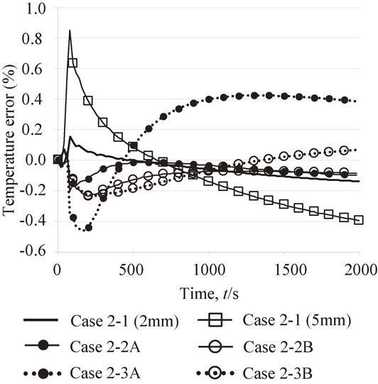
Error of cooling curve at A using ARPM.
The time-averaged error of cooling curve Eave (K/s) at each measuring points was summarized in Fig. 12. Eave was calculated using eq. (6). The error was standardized by the initial temperature difference, 1530 K, which appeared in the denominator.
| \begin{equation} E_{ave} = \frac{\displaystyle\sum_{l}|T_{i} - T_{\text{$\mathit{Case}$2-1(1$\mathit{mm}$)}}|}{1530t_{\textit{sol}}} \end{equation} | (7) |

Average temperature error of cooling curve at each measuring points.
Here, TCase2-1(1mm) is the temperature in the case 2-1 (1 mm). Figure 12(a) is the results in the case 2-1. tsol = 2000 s was used uniformly in eq. (6). We can see the tendency that the smaller element size showed the smaller error at all points, and the largest error was observed at the point A for all element size. Figure 12(b) is the results using ARPM. The case 2-2 shows very small error, and case 2-3 shows relatively larger error, but the values were still smaller than those of case 2-1 (5 mm).
The point E is the center of the casting, and showed a little larger error than points C and D in the case 2-1. On the other hand, the error at the point E was smaller than those at C and D in the case 2-2 and 2-3 using ARPM.
These series of results show that the temperature error at the measuring points increases with decreasing the number of layers from the casting-mold interface at which a large temperature drop is easy to occur. However, we must be careful that the accuracy of solidification simulation should not be discussed only with the temperature error. Larger element around the interface is easy to decrease its temperature at the very early stage of the calculation, however, the temperature gradient is also easy to decrease. Both characteristic behavior influence on the accuracy of temperature calculation, and the series of results in this section were the summary of such effects. Therefore, solidification time and heat conservation ability were discussed in the next section.
4.4 Discussions 4.4.1 Solidification timeFigure 13 shows the calculated solidification time. The results of case 2-1 are the same with those in Fig. 8. Case 2-2A, 2-2B and 2-3B showed similar solidification time, which were equal to that of case 2-1 (2 mm). However, case 2-3A showed shorter time than case 2-1 (1 mm), which was caused by a heat conservation error as discussed in the section 4.3.3. Case 2-3B showed a little larger temperature error (Fig. 12) at the measuring points, however the overall error was still small enough, and the solidification time was almost equal to that of case 2-2 or 2-1 with smaller elements. The series of results show that the calculated temperature at each measuring points has enough accuracy to estimate the cooling curves, however the lower limit of element size should be taken into account to keep energy conservation ability.

Calculated solidification time using ARPM.
Variation of the total enthalpy with time in the system was shown in Fig. 14 to confirm the energy conservation ability. In case 2-1, excellent energy conservation ability was observed. The total enthalpy did not change by the solidification complete when using uniform element size. In the case of ARPM, slight total enthalpy variation was observed. In the case 2-2, the total enthalpy drop at the early stage of calculation, and keep the value around 0.05%. In the case 2-3A, the total enthalpy was lower than that of case 2-2, resulting shorter solidification time. The case 2-3B shows an increase of total enthalpy after dropping at the beginning of the calculation. Generally, an amount of heat flux at larger elements is larger because of its wide interaction area. For example, the heat flux from larger and high temperature element to a far smaller and low temperature element was taken into account at the larger elements, however the flux would not consider at the smaller element if the interaction area is not enough to reach the larger element. Therefore, the heat release from larger elements tend to excess, and heat receive by larger elements also tend to excess. The results of ARPM in Fig. 14 showed the balance of such behavior. Nevertheless, in the past study, a calculated shrinkage shape agreed well with the experimental result whereas the enthalpy error was 0.2%,3) therefore Fig. 14 shows enough accuracy of enthalpy calculation which was equal to that using uniform small size elements. Definitely, the accuracy with moving elements should be investigated in the future works.

Total enthalpy variation.
Figure 15 shows a computational time (tcom) and a breakdown list of the number of calculation elements (N) for each element size. Case 2-1 (2 mm) showed high accuracy, however required a huge amount of elements and computational time, whereas the case 2-1 (5 mm) uses less elements and shorter time. The ARPM required larger computational time compared with the case 2-1 (5 mm), however the amount of elements was much less than the case 2-1 (2 mm) to obtain the similar accuracy. The major factor of long computational time of ARPM is a time increment of each time step, caused by the use of smaller element size. Therefore the efficiency will increase by adaptive time increment for each element size. Also, further improvement of efficiency is expected in the case with the three-dimensional calculation, because the volume ratio of larger parts would increase compared with the two-dimensional model, especially in the case such as die casting process.

Computational time and breakdown list of the number of calculation elements for each element size.
Adaptive resolution particle method (ARPM) was applied to the heat and solidification simulation. As a result, the ARPM showed good accuracy of solidification simulation and improve its efficiency of the computational time and the memory usage, slightly reducing an energy conservation quality.