Multi-Phase-Field Modeling of Transformation Kinetics at Multiple Scales and Its Application to Welding of Steel

Abstract

Production processes of structural materials generally involve a variety of microstructural evolutions, spatiotemporal scales of which are different by several orders of magnitude. In this study, a multi-phase-field model for simulating transformation phenomena at multiple scales is developed by considering mesoscopic kinetics of interest based on diffuse interface description without curvature effect. In particular, the present model is developed for simulations of microstructural evolutions during welding of carbon steels. In this model, the motion of dendrite envelope is described to simulate solidification not at a dendritic scale but at a scale of grain structure. Moreover, the pinning effect is described based on a mean-field approximation, which allows for simulations of grain growth with existence of very fine particles. The present model is applied to two-dimensional simulations for welding processes of carbon steel. The microstructural evolution involving the melting, solidification, austenite grain growth and pinning effect due to very fine particles is demonstrated.

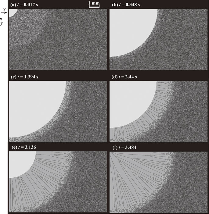
Fig. 8 Microstructural evolution during welding, where the bright region represents the liquid pool in each snapshot. σ_s = 1.0 and f_v was calculated using eq. (19).

1. Introduction

The phase-field method is a method of choice for simulating microstructural evolution processes during various phase transformation phenomena in structural materials.^1–4) It has been applied to simulations of solidification, grain growth in polycrystalline materials, solid-state phase transformations including diffusion-controlled and diffusionless transformations. This is a diffuse interface approach in which the microstructural evolution is characterized by the spatiotemporal variation of phase-field variable(s) and one can thereby avoid explicitly tracking the position of the moving interface. Although phase-field simulations generally require a high computational cost, recent advances in high-performance computing techniques allow for large-scale simulations of microstructures, making this model more powerful and more effective for investigating microstructural phenomena.^5–9)

Most of production processes of structural materials involve several phase transformations that occur simultaneously or sequentially. It is generally straightforward to describe multi-physics problems in the phase-field method, and thereby, several phase transformations, in principle, can be modeled in a single phase-field method. However, spatiotemporal scales for microstructural evolutions are different by several orders of magnitude, depending on the phenomena. To investigate microstructural evolutions in practical production processes, therefore, one needs a model that can describe phenomenon at different scales simultaneously, while such a model has not been developed yet. Welding of carbon steels is one of typical and important problems that require such modeling as described below.

As-solidified weld microstructure is closely related to properties of weld joint.¹⁰⁾ Prediction of growth process of solidifying grains requires detailed description of time evolution of dendrite structures, which is computationally demanding. For instance, when a solidifying grain consists of tens of dendrites, simulations for growth process of tens of solidifying grains require description of time evolution of hundreds of dendrites. It is not straightforward to do such a simulation even with a help of recent high-performance computing technique. Furthermore, austenite (γ) grain growth occurs in a heat affected zone (HAZ) during welding of carbon steels. Since the grain size is an important factor affecting properties of the weld joint, it is important to predict the grain growth accurately. Note that the grain growth is affected by complicated thermal history, and also, grain structures in a partially-melted zone are not independent of the solidification processes in the melted zone. The grain growth process is further compounded when a pinning effect exists. If the size of pinning particle is in the order of nm, spatial resolution for the microstructural simulation needs to be in the order of nm (i.e., the grid spacing of ∼nm). On the other hand, the system size must usually be set to the order of mm to describe microstructural evolutions in regions including melted zone and HAZ. Such a simulation is impossible because of its extremely large computational burden. It is indispensable to develop a model that can describe phenomenon at different scales simultaneously.

The main objective of this study is to develop a phase-field model that can describe kinetics of phase transformations at multiple scales. In standard phase-field models, effect of curvature (Gibbs-Thomson effect) naturally arises in motion of physical interface.^1–4) In this study, motion of diffuse interface without the curvature effect is described to represent motion of boundaries between different regions (region boundary), which enables use of theories for kinetics of phase transformation at different scales. We develop such a model specifically designed to simulate the welding of carbon steels. As mentioned above, prediction of weld microstructure requires simultaneous descriptions of solidification, melting, grain growth and the pinning effect due to fine particles. In this study, the solidification and melting phenomena are modeled not at dendritic scale but at a scale of grain structure (dendrite envelopes) in a way similar to mesoscopic cellular automaton (CA) models for solidification microstructures.^11,12) In addition, the pinning effect due to fine particles is described based on a mean field approximation. The present model is applied to simulations for solidification, grain growth and, in particular, welding process of carbon steel.

Mesoscopic CA models have been applied to simulations of solidification grain structure formed during welding processes^13,14) and simulations of grain growth in polycrystalline materials.^15,16) Hence, one will be able to describe microstructural evolutions in regions including melt zone and HAZ in welding processes by combining such CA approaches. On the other hand, the present model is based on the phase-field model and, thereby, it should be superior to CA-based approaches in that explicit tracking of the position of moving interfaces can be avoided and curvature effects can be precisely calculated because of smooth representation of interface shapes thanks to diffuse interface description.

2. Modeling and Computational Details

2.1 Grain growth

The present model is based on the multi-phase-field (MPF) model.^17,18) This model has successfully been applied to simulations of several phenomena including grain growth in polycrystalline materials. In the MPF model, the grain structure is characterized by a set of phase-field variables, {ϕ_i(r, t)}. The phase-field variable ϕ_i(r, t) (0 ≤ ϕ_i ≤ 1) represents a probability of finding a grain i at the spatial coordinate r and time t. The normalization condition $\sum\nolimits_{i = 1}^{N}\phi _{i} = 1$ is satisfied at each spatial point. Here, N is the total number of grains counted in the simulation. The grain boundary is described as the diffuse interface in which ϕ_i continuously changes from 0 to 1. The time evolution of ϕ_i is described by the following equation;¹⁸⁾   

\begin{equation} \frac{\partial\phi_{i}}{\partial t}=-\frac{2}{S}\sum_{j\neq i}^{N}s_{i}s_{j}M_{ij}\left[\frac{\delta F}{\delta\phi_{i}}-\frac{\delta F}{\delta\phi_{j}}\right] \end{equation} (1)

where   

\begin{equation} \frac{\delta F}{\delta\phi_{i}}=\sum_{k\neq i}^{N}\left[\frac{\varepsilon_{ik}}{2}\nabla^{2}\phi_{k}+\omega_{ik}\phi_{k}\right] \end{equation} (2)

Here, s_i is the step function associated with ϕ_i, which takes 0 for ϕ_i = 0 and takes 1 for ϕ_i > 0. S is given as $S = \sum\nolimits_{i = 1}^{N}s_{i} (\mathbf{r},t)$. M_ij, ε_ij and ω_ij are the phase-field mobility, the gradient energy coefficient and potential height, respectively, between the grains i and k. In this study, we do not consider dependence of grain boundary properties on types of grains, that is, our focus is placed on an isotropic system. Therefore, M_ij = M, ε_ik = ε and ω_ik = ω. When the grain boundary energy and thickness are indicated by σ_gb and W, ε and ω are given as $\varepsilon = 2\sqrt{2W\sigma _{gb}} /\pi $ and ω = 4σ_gb/W, respectively.

Equation (1) is reduced to the relation, v_gb = −Mε²κ, where v_gb is the grain boundary velocity, κ is the local curvature of the grain boundary. Hence, the curvature-driven growth is described in this model. In this study, the following relation is employed,   

\begin{equation} M=\frac{m_{gb}\sigma_{gb}}{\varepsilon^{2}} \end{equation} (3)

where m_gb is the grain boundary mobility. Then, we can reproduce the well-known relationship for curvature-driven growth¹⁸⁾ as follows,   

\begin{equation} v_{gb}=-m_{gb}\sigma_{gb}\kappa=-k_{gb}\kappa \end{equation} (4)

where k_gb = m_gbσ_gb can be determined from time change of average grain size. In this study, we assume the following form for k_gb,   

\begin{equation} k_{gb}=k_{gb}^{0}\exp\left(-\frac{Q}{\mathit{RT}}\right) \end{equation} (5)

Here, k_gb⁰ and Q are constants. Experimental investigations on isothermal grain growth often find   

\begin{equation} \langle R\rangle^{2}-\langle R_{0}\rangle^{2}=K_{gb}^{\text{exp}}t \end{equation} (6)

where ⟨R⟩ is the average grain radius, ⟨R₀⟩ is its initial value and $K_{gb}^{\text{exp}}$ is a coefficient of temperature-dependent. Then, the following relation is satisfied,   

\begin{equation} K_{gb}^{\text{exp}}=a_{gb}\cdot k_{gb} \end{equation} (7)

where a_gb is a constant which depends on the dimension of the simulation. We found a_gb = 0.322 ± 0.002 from two-dimensional (2D) isothermal grain growth and a_gb = 0.509 ± 0.005 from three-dimensional (3D) isothermal grain growth. Hence, k_gb can be determined from the experimental data on the grain growth.

2.2 Melting and solidification

Quantitative phase-field models have been developed as accurate diffuse interface models for reproducing the solution of free-boundary problem in the thin-interface limit.^19–25) These models have been applied to investigations of a variety of solidification microstructures.^6–9) In particular, multiple dendritic growth with motion, collision and coalescence and the subsequent grain growth has recently been modeled by combining the quantitative phase-field model with the lattice Boltzmann method.²⁶⁾ Therefore, one can employ these models to understand details of formation processes of dendrite structures and the resulting microsegregation.

On the other hand, if details of dendrite structure and the microsegregation are not targets for investigations, one can characterize the solidification by kinetics of region boundary between the liquid region and solid region which consists of dendrites and the interdendritic liquid, instead of describing the detailed motion of physical interfaces, i.e., solid-liquid interface. It allows for description of solidification at a scale larger than the dendritic scale. The kinetics of region boundary can be determined based on the theories of dendritic growth such as Kurz-Giovanola-Trivedi (KGT) model²⁷⁾ or results of the above-mentioned phase-field simulations. This is actually the approach that mesoscopic cellular automaton models are based on.^11,12) In this study, this approach is realized within framework of the MPF model. Note that the curvature effect naturally arises in the motion of diffuse interface in standard phase-field models. However, the region boundary is free from the curvature effect. In this study, therefore, the motion of diffuse interface without the curvature effect is modeled.²⁸⁾ Although our modeling is made for the solidification problem, the present model can be applied to other phase transformations including solid-state phase transformations.

The present model is based on the MPF model described in Sec. 2.1. To describe the solidification (and melting), we introduce the phase-field variable, ϕ_N+1, which represents a probability of finding the liquid phase. The region where ϕ_N+1 = 1 and ϕ_i = 0 with i ≠ N + 1 is the liquid region. The region boundary characterized by 0 < ϕ_N+1 < 1 and ϕ_i = 1 − ϕ_N+1 accordingly correspond to the boundary between the liquid and grain i. Note that this boundary is not the solid-liquid interface at a dendritic scale but the region boundary between the liquid region and solid region which consists of dendrites and the interdendritic liquid (dendrite envelope) at a scale of grain structure. In this study, the time evolution of ϕ_N+1 is described by the following equation;   

\begin{align} \frac{\partial\phi_{N+1}}{\partial t}&=M\biggl(\varepsilon^{2}\nabla^{2}\phi_{N+1}-\omega(1-2\phi_{N+1}) \\ &\quad-\frac{8}{\pi}\sigma_{gb}\sqrt{\phi_{N+1}(1-\phi_{N+1})}\left(\kappa+\frac{F_{\textit{env}}}{M\varepsilon^{2}}\right)\biggr) \end{align} (8)

where κ is the curvature of dendrite envelope as given by κ = ∇ · (∇ϕ_N+1/|∇ϕ_N+1|). Equation (8) was formulated to reproduce the following relation;   

\begin{equation} v_{\textit{env}}=F_{\textit{env}} \end{equation} (9)

where v_env is the moving velocity of dendrite envelope. Therefore, the effect of curvature on the motion of boundary is removed in this model and the kinetics of moving interface is entirely determined by F_env.

In this model, one can choose any expression of F_env suitable for the phenomena of interest. For instance, it can be expressed as a function of undercooling ΔT = T − T_L using the KGT model²⁷⁾ or LKT model.²⁹⁾ Also, it can be described as a function of local temperature and local concentration by using results of phase-field simulations for melting and solidification. For simplicity, in this work, we assume the following relations,   

\begin{equation} F_{\textit{env}}= \begin{cases} \alpha_{m}(\mathbf{n})(A_{m}\Delta T+B_{m}\Delta T^{2}+C_{m}\Delta T^{3}) \\ \quad \textit{for $\Delta T>0$}\\ \alpha_{s}(\mathbf{n})(A_{s}\Delta T+B_{s}\Delta T^{2}+C_{s}\Delta T^{3}) \\ \quad \textit{for $\Delta T\leq 0$} \end{cases} \end{equation} (10)

where A_m, B_m, C_m, A_s, B_s and C_s are constants, α_m(n) and α_s(n) are functions introduced to describe dependences of melting and solidification velocities on the crystal orientation of grain. In cubic crystals such as fcc and bcc, the preferential growth direction of dendrite corresponds to ⟨100⟩, and accordingly, the growth in ⟨100⟩ exhibits the highest velocity. In this study, a_s(n) is defined as follows;³⁰⁾   

\begin{equation} \alpha_{s}(\mathbf{n})=1-\sigma_{s}\left(1-\frac{|\mathbf{n}|_{4}^{4}}{|\mathbf{n}|_{2}^{4}}\right) \end{equation} (11)

where $|\mathbf{n}|_{h} = (\sum\nolimits_{i = 1}^{3}n_{i}^{h} )^{1/h}$ with n_i = ∂ϕ_N+1/∂x_i, σ_s is a parameter controlling the shape of dendrite envelope. In the present simulations, ⟨100⟩ orientation of each grain was described by the Eular angles (y-z-y) and the corresponding coordination rotation was carried out to calculate n_i. The growth of solidifying grain is isotropic when σ_s = 0 (thus α_s(n) = 1), while the growth preferentially occurs in ⟨100⟩ when σ_s > 0. In the latter case, one can describe the orientation-dependence of dendrite tip position and hence σ_s is regarded as a parameter controlling competitive growth between solidifying grains. For simplicity, we assume α_m(n) = α_s(n) in this study.

The focus in this study is to develop a basic framework for dealing with phenomena at multiple scales in the MPF model. Hence, we neglected occurrence of peritectic reaction in carbon steel and used the simple expression for F_env as given by eq. (10). Accurate descriptions for melting and solidification processes require more sophisticated modeling for F_env. Such modeling remains as an important future work. In addition, the nucleation event was not considered in the present study for the sake of simplicity. It is also important to work out how to describe nucleation processes in an accurate manner in the present model.

2.3 Pinning force

The pinning effect on grain growth has been examined using the MPF model.^31,32) In conventional modeling of the pinning effect, pinning particles are explicitly described in the microstructures by using phase-field variable(s) that represents a probability of finding the pinning particles. In doing so, one can directly describe interaction between the moving grain boundary and the pinning particles. However, if the size of pinning particle is much smaller than the grain size, it is virtually impossible to perform the simulation for this process because of extremely large computational burden.

In this study, the pining effect is described based on a mean field approximation. To be more specific, the pinning particles are not explicitly described in the microstructure, and therefore, one can avoid using very fine grid spacing associated with fine pinning particles. Because little has been clarified about pinning effects on triple junction and multiple junctions of grain boundaries, our modeling is limited to pinning effect only on boundaries between two grains as is usual in conventional pinning theories. In this study, the pinning effect is described by solving the following equation,   

\begin{equation} \frac{\partial\phi_{i}}{\partial t}=M\left(\varepsilon^{2}\nabla^{2}\phi_{i}-\omega(1-2\phi_{i})-\frac{8}{\pi}\sqrt{\phi_{i}(1-\phi_{i})}G_{\textit{pin}}\right) \end{equation} (12)

This equation is solved only when S = 2 in eq. (1), while eq. (1) with eq. (2) is solved otherwise. Here, G_pin is given as   

\begin{equation} G_{\textit{pin}}= \begin{cases} -\Delta P_{\textit{pin}} & \textit{for $\kappa>\Delta P_{\textit{pin}}$}\\ \kappa & \textit{for $-\Delta P_{\textit{pin}}\leq\kappa\leq\Delta P_{\textit{pin}}$}\\ \Delta P_{\textit{pin}} & \textit{for $\kappa<-\Delta P_{\textit{pin}}$} \end{cases} \end{equation} (13)

where ΔP_pin represents the mean-field pinning pressure. This model reproduces the well-known relationship in the theory of pinning as follows,³³⁾   

\begin{equation} v_{gb}= \begin{cases} -m_{gb}(\sigma_{gb}\kappa-\Delta P_{\textit{pin}}) \quad \textit{for$\quad\sigma_{gb}\kappa>\Delta P_{\textit{pin}}$}\\ 0 \quad \textit{for$\quad{-}\Delta P_{\textit{pin}}<\sigma_{gb}\kappa<\Delta P_{\textit{pin}}$}\\ -m_{gb}(\sigma_{gb}\kappa+\Delta P_{\textit{pin}}) \quad\textit{for$\quad\sigma_{gb}\kappa<-\Delta P_{\textit{pin}}$} \end{cases} \end{equation} (14)

Note that the phase-field model for pinning effect based on the mean-field approximation was developed using the double-well potential in a recent work.³⁴⁾ Our model for the mean-field pinning force basically corresponds to the extension of their model to the model with the double-obstacle potential.

One can choose a form of ΔP_pin according to the theory or experimental finding for pinning effects. In this study, we define ΔP_pin as follows,³⁵⁾   

\begin{equation} \Delta P_{\textit{pin}}=\sigma_{gb}\beta\frac{f_{v}^{m}}{r_{p}^{n}} \end{equation} (15)

where β is a constant, f_v and r_p are the volume fraction and the average radius of the pinning particle, respectively, and m and n are constants. We assumed the following temperature dependence of f_v,   

\begin{equation} f_{v}=A_{f}+B_{f}T+C_{f}T^{2}+D_{f}T^{3} \end{equation} (16)

where A_f, B_f, C_f and D_f are constants determined from experimental results or thermodynamic calculations. The time change of r_p can be calculated as,   

\begin{equation} \frac{dr_{p}}{dt}=k_{p}(T)\frac{1}{r_{p}^{q}} \end{equation} (17)

where k_p(T) is a kinetic coefficient of temperature-dependent and q is a constant. Although eq. (17) was implemented in our code, we will show results with r_p = constant in this paper.

2.4 Computational details

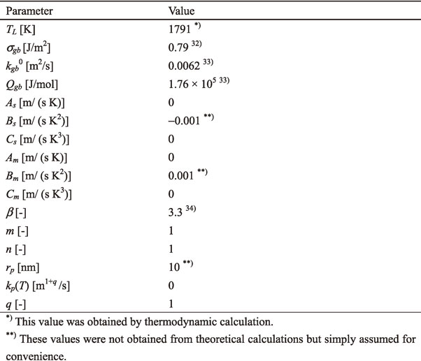
We carried out several simulations to test our model using two-dimensional (2D) systems. Equations (1), (8) and (12) were discretized on the basis of second-order finite difference formulas with a square grid spacing of Δx. The time evolutions were solved using a simple first-order Euler scheme. To simulate coalescence-free grain growth within a reasonable computational time, we employed the active parameter tracking (APT) algorithm.¹⁸⁾ The maximum number of stored phase-field variables in each local grid point was set to 5 in the APT algorithm. In all simulations, the grain boundary thickness W was set to W = 6Δx. In this study, we focus on an Fe–0.15 mass%C–1.5 mass%Mn alloy. The input parameters are listed in Table 1.^36–38) All simulations were accelerated using a TESLA P100 graphics processing unit (GPU).^5–9)

Table 1 Values of parameters used in all simulations of this study.

3. Results and Discussion

3.1 Solidification of single grain

As described in Section 2, the growth of solidifying grains in an undercooled melt can be described in the present model. The shape of grains is controlled by σ_s in eq. (11). We carried out simulations of a single grain growing in an undercooled melt to check the effect of σ_s on the shape of growing solid in this model.

We used a 2D computational system of 1 × 1 mm² and divided it into 1024 × 1024 grid points. Zero Neumann condition was applied to all boundaries. The system initially consists of an undercooled melt and a solid grain with initial radius of 50 µm. The growth of the single particle was simulated.

Figure 1(a) is the initial microstructure where the dark and bright regions are the solid grain and liquid region, respectively. Although not shown here, the solid grain keeps the round shape during isothermal growth when σ_s = 0.0. Figure 1(b) represents the microstructure after isothermal holding for t = 0.0186 s at T = 1786 K (ΔT = −5 K) calculated for σ_s = 1.0. The shape of solid grain is not round but the diamond-like shape. This is the shape of envelope of the growing dendrite, and therefore, the corner of this region corresponds to the orientation of the preferential growth direction, i.e., ⟨100⟩. Figure 1(c) shows the microstructure when the axis of the crystal orientation is rotated by 30° to the left. The diamond-shaped grain is rotated by 30°. Slightly bulged region appears on sides of the diamond, which originates from the numerical inaccuracy related to the finite difference method and can be removed by changing Δx and/or W.

Fig. 1

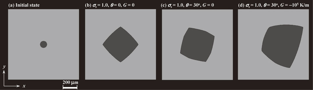
Solid grains growing in an undercooled melt at (a) t = 0 (initial state) and at (b–d) t = 0.0186 s calculated for (b) ΔT = 5 K, σ_s = 1.0, θ = 0°, G = 0, (c) ΔT = 5 K, σ_s = 1.0, θ = 30°, G = 0 and (d) σ_s = 1.0, θ = 30°, G = −10⁴ K/m where the temperature on the left-hand side was set to 1791 K.

The growing shapes shown in Figs. 1(b) and 1(c) are symmetric with respect to ⟨100⟩ axis of each grain because these are the microstructure during isothermal solidification. Figure 1(d) shows the microstructure during solidification under temperature gradient G, calculated for σ_s = 1.0, θ = 30°, G = −10⁴ K/m. The temperature on the left-hand side (right-hand side) was set to 1791 K (1781 K). The shape of growing solid is not symmetric with respect to ⟨100⟩ axis because the driving force for solidification in the right-hand direction is larger than that in the left-hand direction in this case. It was demonstrated in Fig. 1 that the present model can describe the dependences of tip position of dendrites on the orientation of crystal and local solidification conditions, that are very important factors in competitive growth between solidifying grains.¹²⁾

3.2 Directional solidification

Unique to the present model is simultaneous description of melting, solidification and grain growth within a reasonable computational cost. This is illustrated by simulations of directional solidification in this subsection. Furthermore, an effect of σ_s on the microstructural evolution during the directional solidification is investigated.

We employed a 2D computational system of 10 × 3.75 mm² and divided it into 4096 × 1536 grid points. We first carried out simulations for isothermal grain growth starting from a microstructure with randomly distributed solids, until the average grain size reached 15 µm. This microstructure was used as the initial microstructure for simulations of directional solidification. In this study, the following frozen temperature approximation was employed,⁵⁾   

\begin{equation} T=T_{\textit{ref}}+R\cdot t+G\cdot x \end{equation} (18)

where T_ref is the reference temperature, R is the cooling or heating rate and x is the spatial coordinate. In this study, the maximum absolute value of ΔT was set to 20 K. More specifically, ΔT was set to ΔT = −20 (+20) when T is lower (higher) than T_L − 20 (T_L + 20). This was carried out to avoid numerical instability related to extremely high driving forces for solidification and melting. Zero Neumann condition was applied at x-edges, while the periodic boundary condition was employed in y-direction.

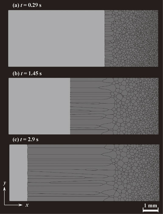
Figures 2(a)–(c) show the microstructural evolution during directional solidification, calculated for T_ref = 1861 K, R = −20 K/s, G = −10⁴ K/m and σ_s = 0.0. The liquid phase was introduced at the origin of the initial microstructure, i.e., ϕ_N+1(0, 0) = 1.0. Hence, melting starts from the origin of this system and takes place in the right-hand direction until t = 0.29 s (Fig. 2(a)). Although not shown here, the grain growth occurs during the melting process. Therefore, the grain structure in Fig. 2(a) is coarser than the initial grain structure. The grain growth also occurs during the subsequent solidification process (Figs. 2(b) and 2(c)). The solidification starts at around t = 0.29 s. The competitive growth between solidifying grains takes place in the left-hand direction from un-melted grains in an epitaxial way, which is followed by formation of columnar grains. Figures 2(a)–(c) illustrate that the melting, solidification and grain growth can be simultaneously described in the present model.

Fig. 2

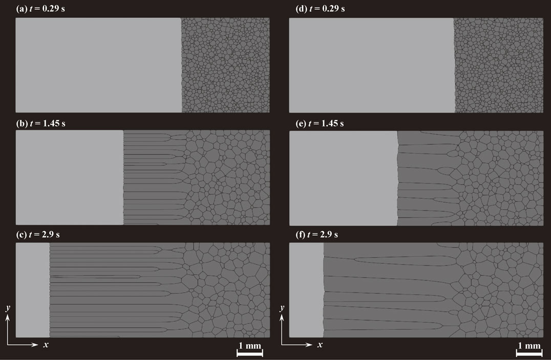
Microstructures during directional solidification at R = −20 K/s and G = −10⁴ K/m at (a, d) t = 0.29 s, (b, e) t = 1.45 s and (c, f) t = 2.9 s, calculated for (a–c) σ_s = 0.0 and (d–f) σ_s = 1.0.

An effect of σ_s on the microstructural evolution is investigated. In the simulations shown in Figs. 2(a)–(c), the solidification velocity is not dependent on the crystal orientation of the grains because of σ_s = 0.0. Figures 2(d)–(f) shows the results for T_ref = 1861 K, R = −20 K/s, G = −10⁴ K/m and σ_s = 1.0. Although the grain structure in un-melted zone away from the melted region is almost the same as that observed in Figs. 2(a)–2(c), a striking difference between results for σ_s = 0.0 (Figs. 2(a)–(c)) and σ_s = 1.0 (Figs. 2(d)–(f)) appears in the columnar grain structure developed by solidification. To be specific, the short-axis diameter of the columnar grains in Fig. 2(f) is much larger that in Fig. 2(c). Since the orientation-dependence of dendrite tip position is included in the simulation with σ_s > 0, grains having ⟨100⟩ almost parallel to x-direction (direction of temperature gradient) preferentially grow to be large in comparison to grains having ⟨100⟩ largely rotated from x-direction. Such a preferential growth process results in large short-axis diameters of columnar grains in Fig. 2(f). Extent of competitive growth is entirely determined by the value of σ_s. It is necessary to find a suitable value for σ_s to reproduce the size of solidified grains quantitatively.

The size of solidified grains also depends on the solidification condition. Figure 3 shows the time evolution of microstructure during directional solidification calculated for T_ref = 2491 K, R = −100 K/s, G = −10⁵ K/m and σ_s = 1.0. From comparison between Figs. 2(d)–(f) and Figs. 3(a)–(c), it is understood that the short-axis diameter of solidified grains decreases by increasing the temperature gradient, G. In other words, selection of solidifying grains requires long-distance solidification when G is large, which is in qualitative agreement with reported experimental observations and model simulations.³⁹⁾

Fig. 3

Microstructures during directional solidification at R = −100 K/s and G = −10⁵ K/m at (a) t = 0.29 s, (b) t = 1.45 s and (c) t = 2.9 s, calculated for σ_s = 1.0.

Several studies have recently been carried out to elucidate formation behaviors of converging and diverging grain boundaries composed of favorably-oriented dendrites and unfavorably-oriented dendrites by means of quantitative phase-field simulations.^6,7,40,41) Reproducibility of these recent findings depends on the validity of F_env. This point remains to be investigated in a future work.

3.3 Pinning effect

The present model reproduces the well-known relationship for pinning effect, eq. (14).³³⁾ We conducted some simulations for pinning effect to test the present model as described below.

For simulations of pinning effect, we employed a 2D computational system of 10 × 7.5 mm² and divided it into 2048 × 1536 grid points. The initial microstructure was prepared by performing simulations of isothermal grain growth starting from randomly distributed solids until the average grain size reached 20 µm. In the simulations for isothermal processes, the periodic boundary condition was applied to all boundaries. In the simulations for grain growth under temperature gradient in x-direction, the periodic boundary condition was applied in y-direction, while zero Neumann condition was applied in x-direction. In all simulations shown here, the radius of pinning particle was set to the constant value of 10 nm for simplicity.

Figure 4(a) shows the snapshot of grain structure after isothermal holding at 1473 K for 11.6 s, calculated with f_v = 0.0, i.e., without the pinning effect. The average grain size increases to about 120 µm from the initial radius of 20 µm in this case. Figures 4(b) and 4(c) represent the grain structures calculated with f_v = 10⁻⁵ and 10⁻³, respectively. The annealing condition is the same as the one in Fig. 4(a). The average grain size gradually decreases with increasing f_v. In case of f_v = 10⁻³, the grain growth hardly occurred because of the strong pinning force.

Fig. 4

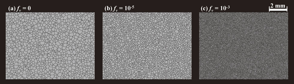
Austenite grains structures after annealing at 1473 K for 11.6 s, calculated for r_p = 10 nm and (a) f_v = 0.0, (b) f_v = 10⁻⁵ and (c) f_v = 10⁻³. The initial value of average grain radius was 20 µm.

Time dependences of average grain radius calculated for different f_v are shown in Fig. 5. Although not explicitly shown, the average grain size exactly follows the parabolic relation, eq. (6), when f_v = 0.0. However, the growth rate gradually decreases with increase in f_v, causing deviations from the parabolic relation. These results indicate that one can describe the pinning effect using the present model. A future work should be aimed at clarifying the detailed nature of pinning effect such as the critical radius for complete pinning and occurrence of abnormal grain growth described by the sharp-interface relation, eq. (14).

Fig. 5

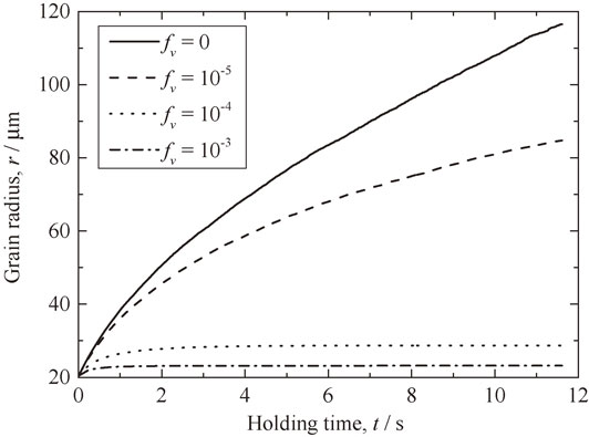
Time dependence of average grain size calculated for f_v = 0, 10⁻⁵, 10⁻⁴ and 10⁻³.

One can consider the temperature dependence of f_v as given by eq. (16). An example of such a simulation is demonstrated. For simplicity, instead of focusing on a specific pinning phase, we consider a model case in which f_v(T) is assumed as follows,   

\begin{equation} f_{v}(T)= \begin{cases} 1.757\cdot 10^{-3}-1.125\cdot 10^{-6}T & \textit{for}\quad\text{$T<1553\,$K}\\ 0 & \textit{for}\quad\text{$T\geq 1553\,$K} \end{cases} \end{equation} (19)

The calculated result of eq. (19) is shown in Fig. 6. Using eq. (19), we conducted simulations of grain growth under the temperature gradient, the initial microstructure of which corresponds to the one employed in simulations of Fig. 4. Figure 7(a) shows the grain structure at 11.6 s calculated for f_v = 0.0. The temperature at the left-hand edge was set to 1573 K and the temperature gradient G was set to G = −10⁴ K/m. Non-uniformity of grain size appears in Fig. 7(a) due to the temperature dependence of grain boundary mobility. The grain size in the left-side region is slightly coarser than that in the right-side region. Figure 7(b) shows the grain structure calculated for the same condition except that f_v is given by eq. (19). Non-uniformity becomes significant in case of Fig. 7(b). The grains remain to be very fine in the right-side region because the volume fraction of the pinning particle is high in this region.

Fig. 6

Temperature dependence of volume fraction of pinning particle calculated by eq. (19).

Fig. 7

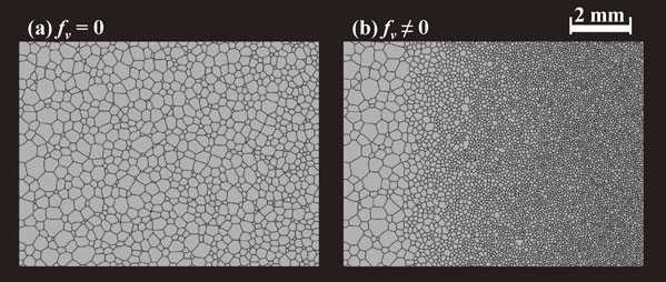
Austenite grain structure after annealing for 11.6 s at G = −10⁴ K/m where the temperature at the left-hand edge was set to 1573 K. (a) f_v = 0 and (b) f_v calculated by eq. (19).

The pinning particles are explicitly described in conventional MPF approaches for the pinning effect. Hence, when r_p = 10 nm, Δx must be in the order of nm. Then, the simulation of growth process shown in Fig. 7(b) requires the grid points of about 10¹⁴ and it is not possible to do such a simulation using standard computational resources.

3.4 Welding

Welding of carbon steels is one of typical processes involving phenomena at multiple scales. In simulations for welding of carbon steels, we need to describe the melting, solidification and grain growth including the pinning effect simultaneously in a system of several mm in length. As an example of application of the present model, we demonstrate the simulation of the welding process.

We employed a 2D computational system of 10 × 6.25 mm² and divided it into 4096 × 2560 grid points. The initial microstructure was prepared by performing simulations of isothermal grain growth starting from randomly distributed solids until the average grain size reached 15 µm. Note that our focus is the process above Ac₃ temperature and this initial microstructure corresponds to the austenite grain structure that forms just above Ac₃ temperature. In the simulations, zero Neumann boundary condition was applied to all boundaries. In this study, the temperature field was calculated based on the following analytical solution for mobile heat source,⁴²⁾   

\begin{equation} T(x,y)=T_{0}+\frac{Q_{\textit{in}}}{2\pi\lambda_{T}r}\exp\biggl(-V_{\textit{weld}}\frac{z'+r}{2a_{\textit{Th}}}\biggr) \end{equation} (20)

  

\begin{equation} r=\sqrt{ {(x-x_{0})^{2}+(y-y_{0})^{2}+z'^{2}}\mathstrut} \end{equation} (21)

  

\begin{equation} z'=-V_{\textit{weld}}t-z_{0} \end{equation} (22)

where T₀ is the preheated temperature, V_weld is the weld velocity, Q_in is the heat input multiplied by V_weld, λ_T is the thermal conductivity, a_T is the thermal diffusivity. x₀, y₀ and z₀ represent the initial coordinates of heat source. In this study, we employed T₀ = 298 K, Q_in = 6000 J/m, λ_T = 40 W/(m K), V_weld = 5 × 10⁻³ m/s, a_T = 9 × 10⁻⁶ m²/s, x₀ = y₀ = 0 and z₀ = −1 × 10⁻³ m. The maximum absolute value of ΔT was set to 20 K to avoid numerical instability related to high driving forces for solidification and melting.

The microstructural evolution during the welding process is shown in Fig. 8 where the bright region represents the liquid pool. Here, σ_s = 1.0 was used for calculation of solidification (and also melting) and eq. (19) was employed for calculation of the pinning effect. The heat source is located at the origin of the computational system, i.e., x = 0 and y = 0. The melting accordingly starts from the origin and, at the same time, the grain growth takes place near the fusion line. The melting almost ceases at around t = 1.394 s, followed by the onset of the solidification. The grains near the fusion line are already very coarse, while the grains away from the fusion line remain very fine because of the pinning effect. The solidifying grains competitively grow, leading to the formation of columnar grains. The final microstructure consists of three distinct structures, i.e., the columnar grain structure in the melted region, the coarse grain structure near the fusion line in the un-melted region and the fine grain structure away from the fusion line.

Fig. 8

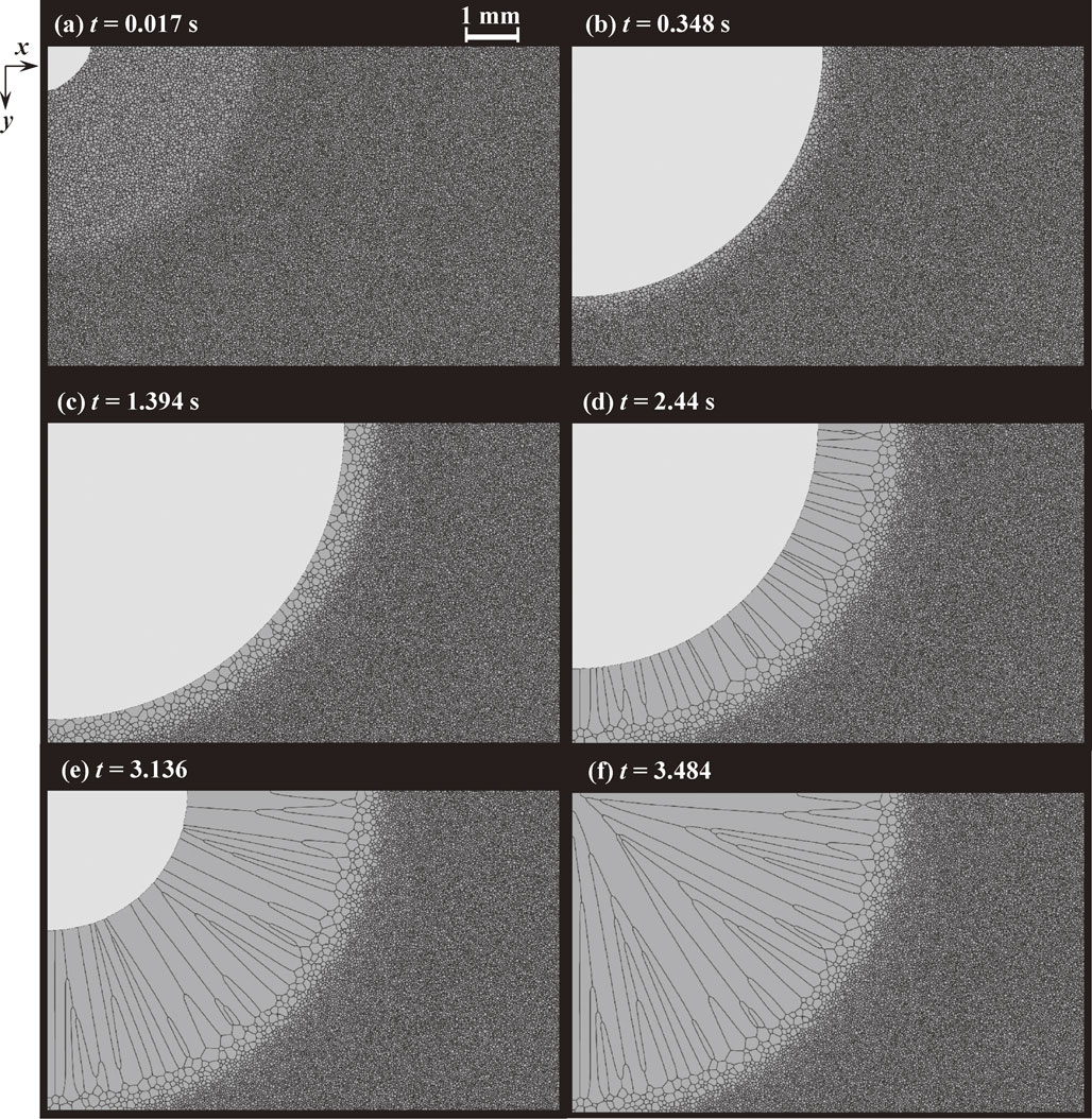
Microstructural evolution during welding, where the bright region represents the liquid pool in each snapshot. σ_s = 1.0 and f_v was calculated using eq. (19).

The microstructural features depend on several factors such as details of competitive growth between solidifying grains, the pinning effect and the thermal history and so on. Figure 9 is the microstructure after welding calculated for the same condition except that σ_s = 0 and f_v = 0. The short-axis diameter of columnar grains in Fig. 9 is shorter than that in Fig. 8 because the preferential growth direction does not exist in the former case. In addition, the microstructure in the un-melted zone gradually changes from coarse grains to fine grains as the distance gets away from the fusion line, which is in contrast with the sharp variation of grain structure from coarse grains to fine grains in Fig. 8.

Fig. 9

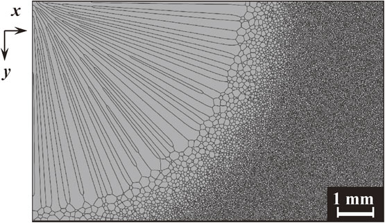
Microstructure after welding, calculated for σ_s = 0 and f_v = 0.

Let us stress that it is virtually not possible to simulate the microstructural evolution process shown in Fig. 8 based on the conventional phase-field model because it requires extremely large computational burden. In this work, we conducted only 2D simulations for the purpose of illustrating outcome of the present model. However, one can carry out 3D simulations of the present model with a reasonable computational burden. 3D simulations must be performed for quantitative discussion in a future work. Furthermore, inclusions of effects of peritectic reaction and nucleation processes are important issues to be tackled in a future work.

4. Conclusions

Production processes of structural materials involve several phase transformations that occur simultaneously or sequentially. In general, spatiotemporal scales for microstructural evolutions in such transformations are different by several orders of magnitude. To investigate microstructural evolutions in practical production processes, in this study, we have developed a multi-phase-field model that can describe phenomenon at multiple scales simultaneously. In the present model, the motion of diffuse interface without effect of curvature can be described and hence it can model a variety of kinetics of moving boundaries. In this paper, the motion of dendrite envelope was modeled to describe the solidification not at dendritic scale but at scale of grain structure. Moreover, the pinning effect was introduced based on the mean-field approximation, which allows for simulations of grain growth with existence of very fine particles. In this paper, the present model was applied to simulations of some processes, in particular, welding of carbon steels, which is one of typical processes that require simultaneous description of melting, solidification, grain growth and pinning effect.

Since the main concern in this paper is to develop the MPF model for describing phenomena at multiple scales, we have made only qualitative discussions about numerical results. It is important to develop a sophisticated form of mesoscopic kinetics such as eq. (10) to describe the microstructural processes in a quantitative manner. In this regard, molecular dynamics (MD) simulations have contributed to the elucidation of the interfacial dynamics and properties required for understanding the microstructural processes.⁴³⁾ Furthermore, large-scale MD simulations are now closing the gap in the knowledge between the microstructural and atomistic scales.^44–47) The atomistic simulations are very useful in determining input parameters of the phase-field simulations and also in finding a proper equation for mesoscopic kinetics in the present model. Hence, these recent progresses will contribute to a further refinement of the present model.

Acknowledgments

This work was supported by Council for Science, Technology and Innovation (CSTI), Cross-ministerial Strategic Innovation Promotion Program (SIP), “Structural Materials for Innovation, Materials Integration” (Funding agency: JST). This research was partly supported by a Grant-in-Aid for Scientific Research (B) (JSPS KAKENHI Grant No. 17K18965) from Japan Society for the Promotion of Science (JSPS). It was also supported in part by MEXT as a social and scientific priority issue (Creation of new functional devices and high-performance materials to support next-generation industries) to be tackled using the post-K computer. The authors wish to thank Prof. Toshiyuki Koyama, Prof. Akinori Yamanaka, Prof. Junya Inoue and Prof. Toshihiko Koseki for stimulating discussions and for providing valuable comments on the present work.

REFERENCES

• 1)   W.J.  Boettinger,  J.A.  Warren,  C.  Beckermann and  A.  Karma: Annu. Rev. Mater. Res. 32 (2002) 163–194.
• 2)   I.  Steinbach: Model. Simul. Mater. Sci. Eng. 17 (2009) 073001.
• 3)  N. Provatas and K. Elder: Phase-Field Methods in Materials Science and Engineering, (Wiley-VCH, New York, 2010).
• 4)   T.  Takaki: ISIJ Int. 54 (2014) 437–444.
• 5)   T.  Takaki,  T.  Shimokawabe,  M.  Ohno,  A.  Yamanaka and  T.  Aoki: J. Cryst. Growth 382 (2013) 21–25.
• 6)   T.  Takaki,  M.  Ohno,  T.  Shimokawabe and  T.  Aoki: Acta Mater. 81 (2014) 272–283.
• 7)   T.  Takaki,  M.  Ohno,  Y.  Shibuta,  S.  Sakane,  T.  Shimokawabe and  T.  Aoki: J. Cryst. Growth 442 (2016) 14–24.
• 8)   T.  Takaki,  S.  Sakane,  M.  Ohno,  Y.  Shibuta,  T.  Shimokawabe and  T.  Aoki: Acta Mater. 118 (2016) 230–243.
• 9)   Y.  Shibuta,  M.  Ohno and  T.  Takaki: JOM 67 (2015) 1793–1804.
• 10)   S.A.  David and  J.M.  Vitek: Int. Mater. Rev. 34 (1989) 213–245.
• 11)   M.  Rappaz and  Ch.-A.  Gandin: Acta Metall. Mater. 41 (1993) 345–360.
• 12)   Ch.-A.  Gandin and  M.  Rappaz: Acta Metall. Mater. 42 (1994) 2233–2246.
• 13)   S.  Chen,  G.  Guillemot and  Ch.-A.  Gandin: Acta Mater. 115 (2016) 448–467.
• 14)   W.  Tan and  Y.C.  Shin: Comput. Mater. Sci. 98 (2015) 446–458.
• 15)   Y.  Liu,  T.  Baudin and  R.  Penelle: Scr. Mater. 34 (1996) 1679–1683.
• 16)   S.  Raghavan and  S.S.  Sahy: Mater. Sci. Eng. A 445–446 (2007) 203–209.
• 17)   I.  Steinbach and  F.  Pezzolla: Physica D 134 (1999) 385–393.
• 18)   S.G.  Kim,  D.I.  Kim,  W.T.  Kim and  Y.B.  Park: Phys. Rev. E 74 (2006) 061605.
• 19)   A.  Karma and  W.-J.  Rappel: Phys. Rev. E 57 (1998) 4323–4349.
• 20)   M.  Ohno and  K.  Matsuura: Phys. Rev. E 79 (2009) 031603.
• 21)   M.  Ohno and  K.  Matsuura: Acta Mater. 58 (2010) 5749–5758.
• 22)   M.  Ohno and  K.  Matsuura: Acta Mater. 58 (2010) 6134–6141.
• 23)   M.  Ohno: Phys. Rev. E 86 (2012) 051603.
• 24)   M.  Ohno,  T.  Takaki and  Y.  Shibuta: Phys. Rev. E 93 (2016) 012802.
• 25)   M.  Ohno,  T.  Takaki and  Y.  Shibuta: Phys. Rev. E 96 (2017) 033311.
• 26)   T.  Takaki,  R.  Sato,  R.  Rojas,  M.  Ohno and  Y.  Shibuta: Comput. Mater. Sci. 147 (2018) 124–131.
• 27)   W.  Kurz,  B.  Giovanola and  R.  Trivedi: Acta Metall. 34 (1986) 823–830.
• 28)   T.  Takaki and  J.  Kato: Mech. Eng. J. 4 (2017) 16-00462.
• 29)   J.  Lipton,  W.  Kurz and  R.  Trivedi: Acta Metall. 35 (1987) 957–964.
• 30)   R.  Kobayashi: Exp. Math. 3 (1994) 59–81.
• 31)   N.  Moelans,  B.  Blanpain and  P.  Wollants: Acta Mater. 53 (2005) 1771–1781.
• 32)   Y.  Suwa,  Y.  Saito and  H.  Onodera: Scr. Mater. 55 (2006) 407–410.
• 33)   M.  Hillert: Acta Metall. 13 (1965) 227–238.
• 34)   S.  Shahandeh and  M.  Militzer: Philos. Mag. 93 (2013) 3231–3247.
• 35)   P.A.  Manohar,  M.  Ferry and  T.  Chandra: ISIJ Int. 38 (1998) 913–924.
• 36)   E.D.  Hondros: Proc. R. Soc. London A 286 (1965) 479–498.
• 37)   C.  Bernhard,  J.  Reiter and  H.  Presslinger: Metall. Mater. Trans. B 39 (2008) 885–895.
• 38)   G.  Couturier,  R.  Doherty,  C.  Maurice and  R.  Fortunier: Acta Mater. 53 (2005) 977–989.
• 39)   H.  Esaka,  K.  Fujita,  H.  Daimon,  M.  Tamura and  K.  Shinozuka: J. Japan Inst. Metals 64 (2000) 1206–1211.
• 40)   C.  Guo,  J.  Li,  H.  Yu,  Z.  Wang,  X.  Lin and  J.  Wang: Acta Mater. 136 (2017) 148–163.
• 41)   T.  Takaki,  S.  Sakane,  M.  Ohno,  Y.  Shibuta,  T.  Aoki and  Ch.-A.  Gandin: Materialia, in press (doi:10.1016/j.mtla.2018.05.002).
• 42)   D.  Rosenthal: Trans. ASME 68 (1946) 849–866.
• 43)   Y.  Shibuta,  K.  Oguchi and  M.  Ohno: Scr. Mater. 86 (2014) 20–23.
• 44)   Y.  Shibuta,  S.  Sakane,  T.  Takaki and  M.  Ohno: Acta Mater. 105 (2016) 328–337.
• 45)   Y.  Shibuta,  S.  Sakane,  E.  Miyoshi,  S.  Okita,  T.  Takaki and  M.  Ohno: Nat. Commun. 8 (2017) 10.
• 46)   S.  Okita,  E.  Miyoshi,  S.  Sakane,  T.  Takaki,  M.  Ohno and  Y.  Shibuta: Acta Mater. 153 (2018) 108–116.
• 47)   Y.  Shibuta,  M.  Ohno and  T.  Takaki: Adv. Theory Simul., in press (doi:10.1002/adts.201800065).