Prediction of Fatigue Strength in Steels by Linear Regression and Neural Network

Abstract

This paper examines machine learning methods to predict fatigue strength with high accuracy using existing database. The fatigue database was automatically classified by hierarchical clustering method, and a group of carbon steels was selected as a target of machine learning. In linear regression analyses, a model selection was conducted from all possible combinations of explanatory variables based on cross validation technique. The derived linear regression model provided more accurate prediction than existing empirical rules. In neural network models, local and global sensitivity analyses were performed and the results of virtual experiments were consistent with existing knowledge in materials engineering. It demonstrated that the machine learning method provides prediction of fatigue performance with high accuracy and is one of promising method to accelerate material development.

1. Introduction

Structural materials are mostly used for a long time and the time-dependent performances such as fatigue, creep and corrosion are directly related to the safety of our infrastructure. As a demand of new materials for specific applications increases and the cost of the experiments to evaluate the time-dependent performances rises, it is becoming increasingly important to reduce the number of experiments in the material development process. Against such a background, many attempts have been made to develop a methodology for predicting the fatigue performances by using physical models, numerical simulation, empirical rules and machine learning. In order to capture the complicated relationship between the manufacturing conditions and the performance, it is effective to decompose the material system into four principal elements of process, structure, properties and performance and to create models for each relationship.¹⁾ By integrating these models, the performance prediction can be realized.^2–5) Despite a great deal of effort using computational simulations,^6–8) there is still a lack of models that predict dislocation structure formation and microstructurally small crack growth under cyclic loading, and it is still challenging to develop the methodology to predict the total fatigue life with the current theoretical understanding. The need to bridge models of the elementary processes over different length scales and time scales makes the fatigue prediction more difficult. Although the empirical rules can be one way to obtain the missing models, the present measurement techniques do not provide sufficient data to derive the empirical models for dislocation and crack initiation.

In contrast, vast amounts of data on the process-performance relationship have been accumulated over the years for engineering applications. These data are not helpful for understanding the elementary processes of fatigue but are useful for interpolative prediction of performance within a limited range of materials. With the rapid improvement of computer performance and development of software, numerous machine learning algorithms have been proposed over several decades. In the traditional approach, we must select an appropriate learning algorithm to solve a problem from the set of the numerous algorithms, and choose the explanatory variables from many features in database. This traditional approach has resulted in successful predictions in various fields. In the field of mechanical properties, Mukherjee et al.⁹⁾ proposed a multivariate regression model to predict the hardness of thermo-mechanically treated rebars as a function of chemical composition and tempering parameters. Ozerdem and Kolukisa¹⁰⁾ predicted multiple mechanical properties of copper alloy by using neural network. Collins et al.¹¹⁾ utilized Bayesian neural network to predict tensile properties of Ti–6Al–4V alloys with high accuracy. Also in the case of fatigue prediction, these approaches have been adopted. Malinov et al.¹²⁾ developed neural network models to predict various mechanical properties including fatigue strength for titanium alloys. Agrawal et al.¹³⁾ compared many kinds of machine learning algorithms for the prediction of fatigue strength in steels. Results of these researches showed that the accuracy of the prediction of fatigue strength was lower than that of other mechanical properties such as tensile strength and hardness. This can be explained by the fact that fatigue involves more complex interactions between microstructure, stress and environment than static mechanical properties. A more sophisticated approach is required for fatigue prediction.

The purpose of this paper is to examine machine learning methods suitable for fatigue problems and to predict fatigue strength with high accuracy using existing database. The database contains fatigue properties on various kinds of materials. Since the mechanism of fatigue failure differs from material to material, empirical formulas should be derived separately for each material group. For this reason, the fatigue dataset was automatically classified by hierarchical clustering method, and a group of carbon steels was selected as a target of machine learning. After data preprocessing, there remained 393 samples with 21 explanatory variables such as chemical compositions, process parameters, heat treatment conditions and inclusion parameters, and one objective variable of fatigue strength. In linear regression analyses, a model selection was conducted from all possible combinations of explanatory variables based on cross validation technique in order to minimize the prediction error. In neural network models, a suitable network topology and an appropriate activation function were examined. Comparing the linear regression and neural network models, the advantage and disadvantage of each model were discussed. Also, by using these models, local and global sensitivity analyses were performed to evaluate the significance of each explanatory variable on the fatigue strength.

2. Methods

2.1 Data

Fatigue data sheet (FDS) provided from national institute of material science (NIMS)¹⁴⁾ was used, which is one of the world’s largest fatigue databases and contains general steels, stainless steels, cast irons, aluminum alloys, nickel alloys, titanium alloys and magnesium alloys. In total, 689 types of metallic materials are linked to the features including fatigue strength, chemical compositions, processing parameters, heat treatment conditions, inclusion parameters and grain size. The chemical composition consists of 25 different elements: Fe, C, Si, Mn, P, S, Ni, Cr, Cu, Mo, Al, N, B, Nb, Ti, W, V, Co, Sb, O, Sn, Mg, Zn, Zr and H. The processing parameters include reduction ratio and heat treatment parameters in pre-heating, normalizing, quenching, tempering, annealing, solution and aging. The inclusion parameters are area fraction of inclusions deformed by plastic work (dA), inclusions occurring in discontinuous arrays (dB) and isolated inclusions (dC). The grain size is recorded for ferrite and prior austenite in several steels, and primary α and transformed β phase of titanium alloy. The fatigue strength was determined at 10⁷ cycles in rotating bending fatigue tests under room temperature.

2.2 Hierarchical clustering and data preprocessing

The fatigue dataset was classified purely based on chemical composition by hierarchical clustering method in order to avoid the artificial categorization. Clustering is one of unsupervised learning methods and classifies data points into different data aggregates, that is, clusters. Among various clustering methods, hierarchical clustering is capable of grouping data points on various scales by creating a dendrogram, and is considered to be effective for classification of metal materials. Hierarchical clustering algorithms are categorized into agglomerative (bottom-up) and divisive (top-down).¹⁵⁾ In the current study, this hierarchical agglomerative clustering was performed with the 689 material samples using the 25 chemical contents as explanatory variables.

It is obvious that the result of the clustering depends on the definitions of distance between data points (intra-cluster distance) and distance between clusters (inter-cluster distance). In order to determine the optimum definitions, clustering analyses were performed with all materials in the database by changing the definitions of intra-cluster and inter-clusters, and it was evaluated whether five kinds of metal materials (iron alloy, aluminum alloys, nickel alloys, titanium alloys and magnesium alloys) can be divided into each cluster. The mean, minimum and maximum values of the parameters used for the clustering analysis is shown in Table 1. Euclidean distance, standardized Euclidean distance and Mahalanobis distance¹⁶⁾ were used as the intra-element distances. Given a dataset comprising n samples of X = (x₁, x₂, …, x_n)^T and each sample has p explanatory variables x_i = (x_i1, x_i2, …, x_ip)^T, the distances between the data points x_i and x_j are defined as follows:   

\begin{equation} d_{ij}^{\text{Euclid}} = \sqrt{\sum_{k = 1}^{p}(x_{ik} - x_{jk})^{2}}, \end{equation} (1)

  

\begin{equation} d_{ij}^{\text{standard Euclid}} = \sqrt{\sum_{k=1}^{p}\left(\frac{x_{ik} - x_{jk}}{\sigma_{k}}\right)^{2}}, \end{equation} (2)

  

\begin{equation} d_{ij}^{\text{Mahalanobis}} = \sqrt{(\mathbf{x}_{i} - \mathbf{x}_{j})\Sigma^{-1}(\mathbf{x}_{i} - \mathbf{x}_{j})^{\text{T}}}, \end{equation} (3)

where σ_k is the standard deviation of feature k, C is the covariance matrix of the entire data X. The inter-cluster distance was calculated by shortest distance method, farthest distance method,¹⁷⁾ group average method,¹⁸⁾ Ward’s method¹⁹⁾ and centroid distance method.²⁰⁾ In the shortest distance method, the distance between the closest two data points belonging to two clusters is measured. Conversely, the farthest distance method uses the distance between the most distant two data points. The group average method uses an average value of distances for all the combinations of two data points belonging to two clusters. The Ward’s method merges the clusters to minimize the difference between the variance of the cluster after merging and the sum of variance of clusters before merging. The centroid method uses the distance between the centroids of clusters. Using three intra-cluster distances and five inter-cluster distances, clustering analyses were performed with a total of 15 algorithms. To assess the quality of the clustering, entropy was calculated for five clusters derived by each algorithm. The entropy of cluster, H, was defined by the following equation:   

\begin{equation} [p_{1},p_{2},\ldots,p_{K}] = \left[\frac{|C(k,1)|}{|C(k)|},\ldots,\frac{|C(k,K)|}{|C(k)|}\right], \end{equation} (4)

  

\begin{equation} H(C(k)) = -\sum_{k = 1}^{K}p_{k}\log p_{k}, \end{equation} (5)

where k is cluster index, K is number of clusters (K = 5), |C(k)| is the number of data points belonging to cluster k, |C(k, j)| is the number of data points corresponding to material j (iron alloy, aluminum alloys, etc.) in cluster k. Low entropy indicates high quality clustering.¹⁵⁾ The total entropy of five clusters was compared among the algorithms to determine the optimal definitions of intra-cluster distance and inter-cluster distance.

Table 1 Mean, minimum and maximum values of explanatory variables used for clustering analysis.

Using the determined definitions of distances, 630 types of iron alloys in the database were clustered. In the NIMS fatigue data sheet, iron alloys are classified into 15 categories of bearing steel, carbon steel for machine structural use, carbon steel for pressure vessels, Cr steel, Cr–Mo steel, Cr–Mo–V steel, ferritic heat-resisting steel, heat-resisting steel, Mn steel, Ni–Cr steel, Ni–Cr–Mo steel, spring steel, stainless steel, tool steel and spheroidal graphite cast iron. To compare with these categories, the maximum number of clusters was set to 15. As the details are to be mentioned in section 3.1, 509 types of steels were classified into one cluster, and were used in the following data preprocessing.

2.3 Data preprocessing

In the fatigue database, not all features exist for all materials. In order to reduce the number of explanatory variables and not to reduce the number of material samples as much as possible, the data was preprocessed as follows:

1. (1)    Alloying elements whose content is 0 mass% in all 630 steels were excluded from the explanatory variables.
2. (2)    Material samples subjected to heat treatment other than quenching, tempering and normalizing were excluded. These three heat treatments have two variables of temperature T (K) and time t (min). These two variables were summarized into one variable of T log(t). For materials not quenched or tempered, T log(t) = 0 was assigned.
3. (3)    The grain size of ferrite and austenite were excluded from the explanatory variables because only either of them was recorded in the most cases. Since primary α and transformed β phase of titanium alloy do not exist in steels, they were excluded.

After the preprocessing, there remained 21 explanatory variables of reduction ratio, dA, dB, dC, Fe, C, Si, Mn, P, S, Ni, Cr, Cu, Mo, Al, N, Ti, O, normalizing, quenching and tempering. The number of materials was 393. The mean, maximum, and minimum values of each explanatory variable are shown in Table 2. These 393 samples were randomly divided into training dataset with 360 samples and test dataset with 33 samples to evaluate the accuracy of linear regression model.

Table 2 Mean, minimum and maximum values of explanatory variables used for training, validation and testing. The fifth column represents selected variables and coefficient a_i of linear regression model.

2.4 Linear regression model

Linear regression is one of the simplest and powerful regression method in which the relationship between explanatory and objective variables is modelled by a linear equation. Multivariate linear regression model can be expressed as follows:   

\begin{equation} y = \sum_{i}^{p}a_{i}x_{i}, \end{equation} (6)

where y is objective variable, x_i is explanatory variable and a_i is constant coefficient for explanatory variables x_i. Although more complex model gives more accurate prediction in the training dataset, if the model is too complex, the accuracy in the validation dataset decrease due to over-fitting.²¹⁾ To avoid this problem, a variable selection from all 2²¹ − 1 combinations of explanatory variables was conducted to minimize the validation error based on cross validation technique. The procedure of the cross validation is illustrated in Fig. 1. At first, 360 training samples were divided for every ten into 36 groups. Linear regression coefficients were calculated for 35 groups except the first group and fatigue strength of first group was predicted by using these coefficients. Then, root mean squared error (RMSE) of this prediction was calculated. After that, 35 groups except the second group were used to calculate coefficients and RMSE was calculated for the second groups. Repeating these procedures, 36 values of RMSE were calculated and total RMSE was recorded as cross validation error (CVE). The cross validation was performed for all 2²¹ − 1 combinations of explanatory variables.

Fig. 1

Schematic representation of the cross-validation method.

2.5 Neural network model

2.5.1 Architecture

Artificial neural network is one way of machine learning which is inspired by biological neural networks. The architecture of artificial neural network used is depicted in Fig. 2(a). In each unit of hidden and output layers, calculation was conducted as following equation and the result was sent to next layer.   

\begin{equation} h_{j} = \varphi\left(\sum_{k}w_{jk}x_{k} + b_{j}\right), \end{equation} (7)

where x_k is the input variable from kth unit in input layer, w_jk and b_k are weight and bias, h_j is the output variable, and φ is activation function. Changing the training algorithms, data normalization method, activation function and number of hidden layers (one or two layers), the prediction accuracy in the test dataset was compared. The number of units in each layer was fixed to be ten units on the first hidden layer and five units on the second hidden layer.

Fig. 2

(a) Architecture of artificial neural network and (b) activation functions.

2.5.2 Activation function

In the output layer, identity function φ(x) = x was used as activation function. In hidden layers, three kinds of non-linear function were used as shown in the following equations and Fig. 2(b):   

\begin{equation} \varphi(x) = \frac{1}{1 + e^{-x}}, \end{equation} (8)

  

\begin{equation} \varphi(x) = \tanh(x) = \frac{e^{x} - e^{-x}}{e^{x} + e^{-x}}, \end{equation} (9)

  

\begin{equation} \phi(x) = \max(0,x). \end{equation} (10)

Equation (8) represents sigmoid function. It was commonly used early in neural network research because it is simple and easy to differentiate. Equation (9) is a hyperbolic tangent. Glorot and Bordes²²⁾ showed that the hyperbolic tangent is more suitable for neural network than the sigmoid function. Equation (14) is a ramp function. In neural network research, this function is called as “Rectified Linear Unit” or “ReLU.” Glorot and Bengio²³⁾ showed that ReLU is better than the hyperbolic tangent. LeCun et al.²⁴⁾ reported that ReLU is the best activation function as of May 2015.

2.5.3 Data normalization

When using sigmoid function or hyperbolic tangent as the activation function, output value converges to ±1 or 0 as the input value moves far from zero. It means that the significance of input variable is almost eliminated. To solve this problem, the input and output variables should be normalized. In this research, three methods of normalization were examined. The first normalization method (hereinafter called “n1”) is to normalize so that the average becomes zero and the variance becomes one as follows:   

\begin{equation} x'{}_{i} = \frac{x_{i} - \bar{x}}{\sigma}, \end{equation} (11)

where x′_i is the normalized variable, $\bar{x}$ is the mean value and s is standard deviation. LeCun et al.²⁵⁾ suggested that this method was the best for neural network. The second and third method (hereinafter called “n2” and “n3”) are to normalize so that the range of x′_i becomes [0, 1] and [0.1, 0.9], respectively:   

\begin{equation} x'{}_{i} = \frac{x_{i} - x_{\text{min}}}{x_{\text{max}} - x_{\text{min}}}, \end{equation} (12)

  

\begin{equation} x'{}_{i} = 0.1 + (0.9\text{-}0.1) \times \frac{x_{i} - x_{\text{min}}}{x_{\text{max}} - x_{\text{min}}}, \end{equation} (13)

where x_max and x_min are maximum and minimum value of each explanatory variable. Sobhani et al.²⁶⁾ used eq. (13) for the neural network model.

2.5.4 Training algorithm

Training of neural network is to properly set weights and biases. The backpropagation algorithm is one of the most common training methods. At the beginning of training process, random values are assigned to weights and biases. The output value is calculated by using these initial weights and biases. Comparing the output value with experimental value, the bias of the output layer and the weight from the hidden layer are updated. Then, comparing the value of the hidden unit with the previous value, the bias of the hidden layer and the weight from the former layer are updated. In a similar manner, all weights and biases are updated. One cycle that updates weights and thresholds in all layers is called one epoch. Thus, the error in the output layer propagates to the input layer through the network, and hence this method is called as backpropagation.

The goal of the backpropagation is to minimize the error. In general, the error is the sum of squared errors between the predicted value and the actual value. To minimize the sum of squares, many algorithms have been proposed. The gradient descent method and the Gauss-Newton method are popular algorithm to solve this problem. The gradient descent method requires a long time to converge and the Gauss-Newton method converges quickly but can give inaccurate results. Consequently, the Levenberg-Marquardt (LM) method²⁷⁾ which is a combination of the gradient descent method and the Gauss-Newton method was adopted. Training was stopped when either the average error on the training datasets was less than a preset value, Marquardt parameter exceeded 1.0 × 10¹⁰, or the number of epochs exceeded 5000. The dataset was randomly divided into 70% for training, 15% for validation and 15% for testing when using LM method.

To prevent over-fitting, Bayesian framework has been proposed for the training in neural network.²⁸⁾ In the framework, the goal of training is to minimize the function E(w) shown below, instead of sum squared error,   

\begin{equation} E(\mathbf{w}) = \beta E_{D}(\mathbf{w}) + \alpha E_{w}(\mathbf{w}), \end{equation} (14)

  

\begin{equation} E_{D}(\mathbf{w}) = \frac{1}{2}\sum_{k=1}^{n}(y_{k} - o_{k})^{2}, \end{equation} (15)

  

\begin{equation} E_{w}(\mathbf{w}) = \frac{1}{2}\sum_{i}w_{i}{}^{2}, \end{equation} (16)

where y_k is predicted value, o_k is observed value (actual value), w is vector of weights and biases. E_D(w) is an error function similar to the total squared error in LM method. E_w(w) is called a penalty term, which encourages to lower the weights and suppresses over learning. The calculation was performed based on LM method. The coefficients α and β are hyper parameters to control the complexity of model. If β is too large, the degree of freedom of the model becomes large and over-fitting occurs. Conversely, if α is too large, the weights and biases are not fitted to the data. To address this problem, the two parameters were statistically determined by Bayes’ theorem.²⁹⁾ The Bayes’ theorem is represented as follows:   

\begin{equation} p(\mathbf{w},\mathbf{D}) = p(\mathbf{w}|\mathbf{D})p(\mathbf{D}) = p(\mathbf{D}|\mathbf{w})p(\mathbf{w}), \end{equation} (17)

where D is data set. When w is the most probable, p(w|D) becomes maximum. p(w|D) is in proportion to two probabilities:   

\begin{equation} p(\mathbf{w}|\mathbf{D}) \propto p(\mathbf{D}|\mathbf{w})p(\mathbf{w}). \end{equation} (18)

Assuming that these two probabilities are normal distributions,   

\begin{align} p(\mathbf{D}|\mathbf{w}) &= \prod_{k=1}^{n}p(o_{k}|x_{k},\mathbf{w})\\ &= \frac{1}{Z_{D}}\exp\left\{-\frac{1}{2\sigma_{v}{}^{2}}\sum_{k = 1}^{n}(y_{k} - o_{k})^{2}\right\},\\ &= \frac{1}{Z_{D}}\exp\left(-\frac{1}{\sigma_{v}{}^{2}}E_{D}\right) \end{align} (19)

  

\begin{align} p(\mathbf{w}) &= \frac{1}{Z_{w}}\exp\left(-\frac{1}{2\sigma_{w}{}^{2}}\|\mathbf{w}\|^{2}\right) \\ &= \frac{1}{Z_{w}}\exp\left(-\frac{1}{\sigma_{w}{}^{2}}E_{w}\right), \end{align} (20)

  

\begin{equation} p(\mathbf{w}|\mathbf{D}) \propto \frac{1}{Z_{D}Z_{w}}\exp \left\{-\left(\frac{1}{\sigma_{v}{}^{2}}E_{D} + \frac{1}{\sigma_{w}{}^{2}}E_{w}\right)\right\}, \end{equation} (21)

where Z_D and Z_w are constants for normalization, σ_v is the standard deviation of actual output values, and σ_w is the standard deviation of weights and biases. Maximizing p(w|D) is equivalent to minimizing (E_D/σ_v² + E_w/σ_w²). Comparing with eq. (14), two coefficients α and β are determined from the standard deviations. According to MacKay,³⁰⁾ there is no need to prepare validation data in the Bayesian framework. Therefore, the data set were chosen randomly for 85% for training and 15% for testing. These two training algorithm, LM method and LM method with Bayesian framework, were compared.

2.5.5 Evaluation

Training conditions are summarized in Table 3. The training algorithm was evaluated with model 1 and 2 in the table. All nine combinations of the three types of activation function and the three normalization method described in previous sections were compared using model 3 to 11. Since the result varied depending on the data dividing, ten training datasets were prepared by randomly dividing the entire data ten times. Each dataset was named as dataset number 1 to 10. In order to further improve the prediction accuracy, a second hidden layer was added to the selected neural network model (model 12). In each model, epoch number, correlation coefficient between actual value and predicted value of training data, validation data, test data and all data were recorded.

Table 3 Training conditions for neural network models. H1 and H2 represent the number of hidden layers, and LM is Levenberg-Marquardt (LM) method, and LM+Bayes is LM method with Bayesian framework.

2.5.6 Sensitivity analysis

Sensitivity analysis (SA) is to evaluate the contribution of input uncertainty to output uncertainty of model.³¹⁾ The sensitivity is divided into local sensitivity and global sensitivity. The local sensitivity refers to the sensitivity at a fixed point in the parameter space, while global sensitivity refers to an integrated sensitivity over the entire input parameter space.³²⁾ In the linear regression model, the coefficient directly represents the local and global sensitivity, as shown in the eq. (6). In contrast to the linear regression model, weights and biases in neural network model have complicated influences on the sensitivity. The local sensitivity can be evaluated by changing only one of the explanatory variables and fixing remaining variables. Several researchers call the local SA in neural network model as “virtual experiment.”¹¹⁾ However, it does not represent the overall significance of the explanatory variables over the entire data. To evaluate the significance on fatigue strength over a wider range of materials, global SA is required. Using the created neural network model, global SA was performed by combined weight method,³³⁾ fourier amplitude sensitivity test (FAST) method^34,35) and Sobol’ method.^36,37) Also, the local SA was conducted to examine the effect of carbon and manganese contents on the fatigue strength.

3. Results and Discussions

3.1 Hierarchical clustering

Total entropy of five clusters is shown in Fig. 3. Among the three intra-cluster distances of Euclidean, standardized Euclidean, and Mahalanobis distance, five metallic materials were successfully clustered with Euclidean distances. Of the five inter-cluster distances, the shortest distance method, the group average method, and the center of gravity method provided successful clustering. In the centroid method, the dendrogram partially reversed and intersected. This is because the centroid of cluster moved due to cluster merging and the distance between clusters does not monotonically decrease. Based on these results, the shortest distance method with Euclidean distance was used in the subsequent clustering.

Fig. 3

Effect of distance definition on total entropy in hierarchical clustering of metallic materials.

Results of hierarchical clustering of 630 iron alloys into 15 clusters using shortest distance method with Euclidean distance are shown in Fig. 4. The horizontal axis represents the distance in the chemical composition space, that is, dissimilarity of chemical composition. In this analysis, 509 alloys of 630 alloys were classified into one cluster. The cluster contained carbon steels and low-alloy steels with small amounts of Cr, Mn, Mo and Ni. Such classification was quite different from 15 categories in the NIMS fatigue data sheet. It indicated that it is necessary to add the information of heat treatment, microstructure and properties in order to perform clustering matching the existing database.

Fig. 4

Results of hierarchical clustering of iron alloys.

3.2 Linear regression model

Result of variable selection with cross validation method is shown in Fig. 5. The horizontal axis shows the number of explanatory variables, p, and the vertical axis shows the minimum CVE for each number of explanatory variables. It can be seen that CVE reached a minimum at p = 14. Selected variables and calculated coefficients are shown in Table 2. Variables of C, Si, Mn, P, Ni, Cr, Cu, Mo, Al, N, Ti, O, quenching, tempering were selected. All of these variables are selected more than 85 times in the top 100 combinations. The normalized coefficients showed that two heat treatments have great significance on the fatigue strength. Also, the result showed that fatigue strength increases by adding elements of C, Mn and Cu, which is consistent with our existing knowledge of solid solution strengthening, substitutional solid solution strengthening and precipitation hardening. Figure 6 shows the prediction result with experimental fatigue strength. Correlation coefficient and RMSE are shown in Table 4. The model provided more accurate prediction for wider range of materials than previously proposed linear regression model.¹³⁾ These results confirmed that variable selection is necessary for highly accurate prediction of fatigue strength.

Fig. 5

Variable selection by cross validation method with linear regression model.

Fig. 6

Scatter plot of the fatigue strength predicted by the linear regression model.

Table 4 Correlation coefficient and root mean squared error (RMSE) of multivariate linear regression model (MR) and artificial neural network model (ANN).

Thus, the variable combination giving the minimum CVE was found by exhaustive search for all combinations. This method is also effective for comparing with existing empirical rules. Igarashi et al. proposed to plot the density of state of CVE and compare various solutions of variable selection on the density of state.³⁸⁾ They called the method as exhaustive search with density of states (ES-DoS). The state of density for CVE of fatigue strength was plotted in Fig. 7. Several peaks were observed in the state of density. There are few empirical rules for predicting fatigue strength of steels directly from manufacturing conditions. For tensile strength of tempered martensitic steels, Umemoto³⁹⁾ proposed the following equation:   

\begin{align} \sigma_{\text{TS}} &= 1301C + 1089C_{\text{s}} - 38.2\textit{Mn} + 3.90\textit{Ni} \\ &\quad- 0.124d_{\gamma} - 17.5I + 1008, \end{align} (22)

where C_s is solute carbon content, d_γ is prior austenite grain size (µm) and I is tempering parameter. Mukherjee et al.⁹⁾ derived the empirical model for predicting the Vickers hardness of the tempered martensite. The Mukherjee’s model contains 14 alloying elements and 2 tempering parameters. Agrawal et al.¹³⁾ derived a linear regression model of fatigue strength using all the features of NIMS fatigue data sheet. Assuming a linear relationship between fatigue strength, tensile strength and hardness, these existing models were mapped on state of density of CVE (Fig. 7). The solute carbon content and the prior austenite grain size were ignored in the mapping. The position of Umemoto’s model suggested a possibility that the grain size and solute carbon content not present in database are important on the fatigue prediction. Agrawal’s model with 21 explanatory variables showed relatively high accuracy. However, compared with the best model with 14 explanatory variables, the accuracy was much lower. These results also demonstrated the necessity of variable selection.

Fig. 7

Results of exhaustive search with density of state (ES-DoS) for cross validation error of fatigue strength and comparison with existing models.

3.3 Neural network model

In the prediction result of model 1 and 2, the epoch number was 17 and 454, the correlation coefficient (R) of the test dataset was R = 0.9798 and 0.9864, respectively. The training time of LM method with Bayesian inference (model 2) was about five seconds using PC with 2.3 GHz octa cores and 16 GB memory. It was longer than the simple LM method (model 1). From comparison of correlation coefficients for the test dataset, it was confirmed that prediction accuracy improves by adding Bayesian inference to LM method. Therefore, in the following neural network models, LM method with Bayesian inference was used as the training algorithm.

Figure 8 shows correlation coefficient of test dataset for neural network models created by three kinds of activation functions and three kinds of normalization methods. The normalization method is different for each of the three plots. The horizontal axis represents the dataset number. Overall, the correlation coefficient scattered depending on the test dataset. The method of n1–ReLU, n2–Tanh, n3–Tanh showed relatively high correlation coefficients, among which n1–ReLU has the smallest variance of the correlation coefficient. Moreover, in the method of n1–ReLU, the training finished at the smallest epoch number among three activation function. These results agreed with the previous studies. In the normalization method of n2 and n3, the variables are converted so as to fit within a certain range, whereas the normalization method of n1 converts variables so that the average becomes zero. LeCun et al.²⁴⁾ suggested that if the average of the inputs is kept away from zero, the updating of the weight is biased toward a specific direction and the training takes long time. The ReLU function returns zero to the negative input value, and when combined with the normalization method of n1, the output of about half units in the hidden layer becomes zero. According to Glorot et al.,²³⁾ the ReLU function enables sparse representation to invalidate a part of the hidden layer, and suppresses over-fitting by lowering the degree of freedom of the model.

Fig. 8

Correlation coefficient of test dataset for neural network models created by three kinds of activation functions and three kinds of normalization methods: (a) n1, (b) n2 and (c) n3.

To further improve the prediction accuracy, a second hidden layer was added to the neural network model (model 12). The prediction results of a neural network model consisting of two hidden layers and n1–ReLU method is shown in Fig. 9. In the models with single hidden layer (model 9) and double hidden layers (model 12), the epoch number was 112 and 135, the correlation coefficient (R) of the test dataset was R = 0.9886 and 0.9916, respectively. By adding the hidden layer the computation time increased slightly. It should be noted that as the number of hidden layers increases, an activation function is applied many times in the network, the gradient may disappear, and updating of the weight may not succeed. In the case of using the sigmoid function or Tanh, this gradient elimination problem can occur.

Fig. 9

Scatter plot of the fatigue strength predicated by the neural network model with the best performance (model 12).

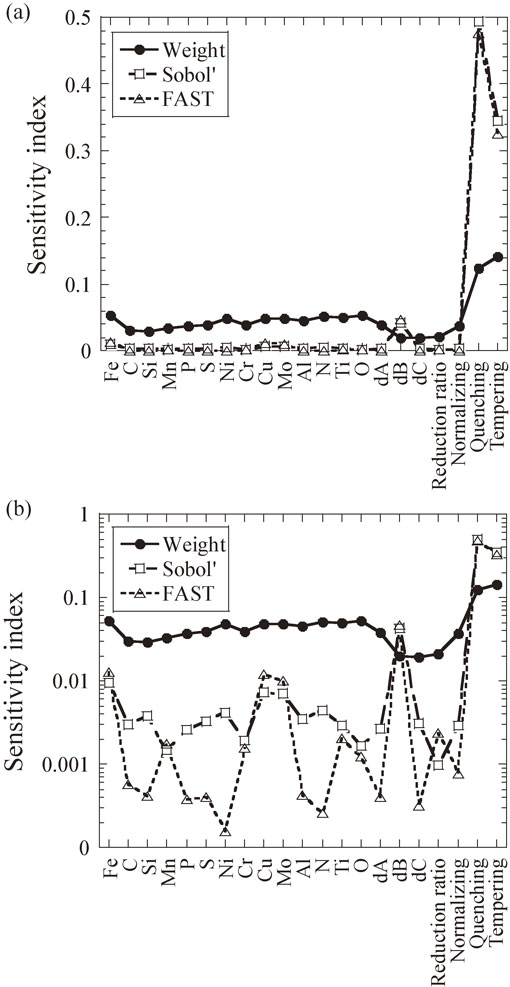
The results of global SA using combined weight method, FAST method and Sobol’ method are shown in Fig. 10. In all three methods, it was shown that quenching and tempering conditions are significant on the fatigue strength. In the combined weight method, not much difference was observed between the sensitivities of alloying elements and inclusions. Whereas FAST method and Sobol’ method showed that the alloying elements of Cu and Mo, and inclusion parameter dB has larger influence on fatigue strength. The dB represents an area fraction of inclusions occurring in discontinuous arrays (Alumina, etc.).

Fig. 10

Results of global sensitivity analyses using model 12 by combined weight method, fourier amplitude sensitivity test (FAST) method and Sobol’ method. The vertical axis represents sensitivity index in (a) linear scale and (b) logarithmic scale.

To examine the effect of carbon and manganese contents on the fatigue strength, local SA (virtual experiment) was conducted by changing C and Mn and fixing the remaining variables to the average value. As shown in Fig. 11, the predicted fatigue strength increased with C and Mn. This result was consistent with known physical phenomena that carbon and manganese exist as interstitial solid solution and substitutional solid solution in steels, respectively, and improve the strength of steels.

Fig. 11

Effect of carbon content on the fatigue strength in two types of steels with different manganese content.

Only the first terms of alloying elements were used in this paper. There is a possibility that the prediction accuracy is further improved by adding lower and higher-order terms of C, and the cross terms between C and carbide-forming elements such as Cr and Mo into the explanatory variables. Also, it is one of promising approaches to select variables by changing combinations of explanatory variables in the neural network models. Since it is difficult to calculate all combinations of 20 or more explanatory variables with neural network models from the viewpoint of computational cost, it may be effective to firstly select variables less than 20 with simple linear regression models and then select the variables in the neural network models.

4. Conclusion

The fatigue dataset provided by NIMS fatigue data sheet was automatically classified by hierarchical clustering method. The shortest distance method with Euclidean distance was suitable for categorizing metallic materials. A group of carbon steels was selected for linear regression and neural network analyses. In linear regression analyses, a model selection was conducted from all possible combinations of explanatory variables, and CVE reached a minimum when the number of variables is 14. It showed that two heat treatments of quenching and tempering have great significance on the fatigue strength. The frequency distribution of CVE in reference to ES-DoS method provided an overview of the relationship between the derived linear regression model and existing empirical rules. In neural network models, the model with double hidden layers, Bayesian framework, ReLU activation function and n1 normalization method provided the best prediction among 12 models. Using the neural network model, local and global SA was performed and the results were consistent with existing knowledge in materials engineering. There is a possibility that the prediction accuracy is further improved by adding lower and higher-order terms and the cross terms into the explanatory variables. These results demonstrated that the machine learning method provides prediction of fatigue performance with high accuracy and is one of promising method to accelerate material development.

Acknowledgments

This work was partially supported by Council for Science, Technology and Innovation (CSTI), Cross-ministerial Strategic Innovation Promotion Program (SIP), “Structural Materials for Innovation” (Funding agency: JST), Japan, and Society for the Promotion of Science KAKENHI (Grant Number 17K14832). The fatigue database used in this study was provided by National Institute for Materials Science (NIMS).

REFERENCES

• 1)   G.B.  Olson: Science 277 (1997) 1237–1242.
• 2)   T.  Koseki: J. Inf. Process. Manage. 59 (2016) 165–171.
• 3)   T.  Koseki: J. Japan Weld. Soc. 86 (2017) 12–15.
• 4)   M.  Enoki: J. Japan Weld. Soc. 86 (2017) 20–23.
• 5)   T.  Shiraiwa,  F.  Briffod and  M.  Enoki: Eng. Fract. Mech. 198 (2018) 158–170.
• 6)   F.  Briffod,  T.  Shiraiwa and  M.  Enoki: Mater. Trans. 57 (2016) 1741–1746.
• 7)   F.  Briffod,  T.  Shiraiwa and  M.  Enoki: Mater. Sci. Eng. A 695 (2017) 165–177.
• 8)   F.  Briffod,  T.  Shiraiwa and  M.  Enoki: Int. J. Fatigue 107 (2018) 72–82.
• 9)   M.  Mukherjee,  C.  Dutta and  A.  Haldar: Mater. Sci. Eng. A 543 (2012) 35–43.
• 10)   M.S.  Ozerdem and  S.  Kolukisa: Mater. Des. 30 (2009) 764–769.
• 11)   P.C.  Collins,  S.  Koduri,  B.  Welk,  J.  Tiley and  H.L.  Fraser: Metall. Mater. Trans. A 44 (2013) 1441–1453.
• 12)   S.  Malinov,  W.  Sha and  J.J.  McKeown: Comput. Mater. Sci. 21 (2001) 375–394.
• 13)   A.  Agrawal,  P.D.  Deshpande,  A.  Cecen,  G.P.  Basavarsu,  A.N.  Choudhary and  S.R.  Kalidindi: Integrating Mater. Manuf. Innov. 3 (2014) 8.
• 14)  Fatigue Data Sheet. National Institute for Materials Science (NIMS). http://smds.nims.go.jp/fatigue, (cited 2018-05-18).
• 15)  M. Steinbach, G. Karypis and V. Kumar: KDD Workshop on Text Mining, (Boston, 2000) pp. 525–526.
• 16)  P.C. Mahalanobis: Proceedings of the National Institute of Sciences (Calcutta), vol. 2, (1936) pp. 49–55.
• 17)   S.C.  Johnson: Psychometrika 32 (1967) 241–254.
• 18)   G.N.  Lance and  W.T.  Williams: Comput. J. 9 (1967) 373–380.
• 19)   J.H.  Ward: J. Am. Stat. Assoc. 58 (1963) 236–244.
• 20)   R.R.  Sokal and  C.D.  Michener: Univ. Kansas Sci. Bull. 28 (1958) 1409–1438.
• 21)  C.M. Bishop: Pattern Recognition and Machine Learning, (Springer-Verlag, New York, 2006) pp. 4–8.
• 22)  X. Glorot and Y. Bengio: Proceedings of the Thirteenth International Conference on Artificial Intelligence and Statistics, Proceedings of Machine Learning Research, PMLR, (2010) pp. 249–256.
• 23)  X. Glorot, A. Bordes and Y. Bengio: Proceedings of the Fourteenth International Conference on Artificial Intelligence and Statistics, Proceedings of Machine Learning Research, PMLR, (2011) pp. 315–323.
• 24)   Y.  LeCun,  Y.  Bengio and  G.  Hinton: Nature 521 (2015) 436.
• 25)  Y. LeCun, L. Bottou, G.B. Orr and K.R. Müller: Neural Networks - Tricks of the Trade, vol. 1524, ed. by G. Orr and K. Müller, (Springer Verlag, 1998) pp. 5–50.
• 26)   J.  Sobhani,  M.  Najimi,  A.R.  Pourkhorshidi and  T.  Parhizkar: Constr. Build. Mater. 24 (2010) 709–718.
• 27)   A.A.  Suratgar,  M.B.  Tavakoli and  A.  Hoseinabadi: World Acad. Sci. Eng. Technol. 6 (2005) 46–48.
• 28)   H.  Fujii,  D.J.C.  Mackay and  H.K.D.H.  Bhadeshia: ISIJ Int. 36 (1996) 1373–1382.
• 29)   H.  Fujii and  K.  Ichikawa: J. Japan Weld. Soc. 70 (2001) 335–339.
• 30)  Bayesian methods for neural networks - FAQ. D.J.C. MacKay. http://www.inference.org.uk/mackay/Bayes_FAQ.html, (cited 2018-05-25).
• 31)   M.  Koda and  T.  Honma: Operations Research as a Management Science Research 55 (2010) 613–621.
• 32)   F.  Cannavó: Comput. Geosci. 44 (2012) 52–59.
• 33)   P.  Hajela and  Z.P.  Szewczyk: Struct. Optim. 8 (1994) 236–241.
• 34)   R.I.  Cukier,  C.M.  Fortuin,  K.E.  Shuler,  A.G.  Petschek and  J.H.  Schaibly: J. Chem. Phys. 59 (1973) 3873–3878.
• 35)   R.I.  Cukier,  J.H.  Schaibly and  K.E.  Shuler: J. Chem. Phys. 63 (1975) 1140–1149.
• 36)   I.M.  Soboĺ: Math. Comput. Simul. 55 (2001) 271–280.
• 37)   I.M.  Soboĺ: Prog. Nucl. Energy 24 (1990) 55–61.
• 38)   Y.  Igarashi,  H.  Takenaka,  Y.  Nakanishi-Ohno,  M.  Uemura,  S.  Ikeda and  M.  Okada: J. Phys. Soc. Jpn. 87 (2018) 044802.
• 39)   M.  Umemoto: Tetsu-to-Hagané 81 (1995) 157–166.