Abstract
Structural adhesives have been used to reduce weight and increase rigidity in recent automotive developments. This study focuses on the fracture behaviors of the cohesive zone under mixed-mode conditions, and a method for evaluation of the J-integral parameters using the displacement of the crack tip opening is proposed. The method is an application of the Dugdale model, which is known as an ideal model to work with a localized plasticity ahead of the crack tip. The validity of the method is verified through finite element analysis. Furthermore, the method is applied to adhesive joints on galvannealed steel, and its fracture mechanism is investigated.
This Paper was Originally Published in Japanese in J. Soc. Mat. Sci., Japan 67 (2018) 1042–1049.
1. Introduction
In recent years, adhesive joints have become an attractive way to fasten structural components in automobile development for reducing weight, increasing rigidity, and multi-materialization.1) At the same time, it is important to quantitatively predict the failure of adhesion joints. The failure mechanisms of adhesive joints can be classified into cohesive failure, in which the adhesive itself is breaks, the failure of the interface between the adherent and the adhesive, the adherent failure, and a mixture of these failures. Until now, several types of testing methods have been widely used for assessing the strength of adhesive joints, such as butt joints and lap joints, and have been defined in ISO standards.2,3) On the other hand, in the case of a defect such as voids or failure of the adhesive end, the above evaluation method is not appropriate, and the evaluation of fracture mechanics is effective. As a method for determining the fracture toughness values of bonded joints, double cantilever beam (DCB) test4,5) in mode I and end notched flexure (ENF) test in mode II are used.6,7) In addition, test methods in the mixed mode are also being studied.8–10) The authors also conducted an experimental study of the adhesion strength against mixed mode for adhesive joints using GA steel sheets (alloyed galvanized steel sheets, Galvannealed Steel) widely used by manufacturers as steel sheets for automobiles.11)
In addition, in recent years, research has been actively carried out to reproduce the fracture behavior of bonded parts considering mixed-mode conditions using a fracture/damage model, such as the cohesion zone model (CZM) incorporated in the general-purpose finite element method software.12–14) For pioneering models of the cohesive zone models, the Dugdale model15) and the Barenblatt model16) for an opening crack and the BCSS model17) for shear crack were proposed. In particular, the Dugdale model estimates the length of the plastic region ahead of the crack tip and the J-integral value from the crack tip opening displacement (CTOD) under mode I loading, assuming that the material is a non-strain-hardened material and that the plastic region is limited to a narrow strip region ahead of the crack tip.18)
In this study, a simple formula for evaluating the J-integral in mixed mode in adhesive joints was proposed based on the Dugdale model. The results of a simple J-integral evaluation formula were compared with a finite-element analysis, and the validity of the proposed formula was confirmed. Furthermore, it was applied to mixed-mode fracture tests of adhesive joints using GA steel plates, and the influence of the mixed mode and thickness of the adhesive layer on the fracture toughness of the bonded joint were investigated.
2. Simple J-Integral Evaluation Formula
2.1 Mixed-mode fracture tests10)
Figure 1 shows the specimens for testing adhesive joints that should be targeted in this study. Two steel plates with dimensions of 40 × 60 × 8 mm were prepared, and GA steel plates with a thickness of 2.3 mm were welded to the long side. An adhesive was applied to the GA steel sheet to make the two steel sheets face each other, and an adhesive joint was formed with a distance between the faces being controlled to be h. At this time, the adhesive was applied on half of the right side, so that a narrow gap remained on the left side, as shown in Fig. 1. The thickness of the adhesive layer was h = 0.3, 0.5, and 1.0 mm.
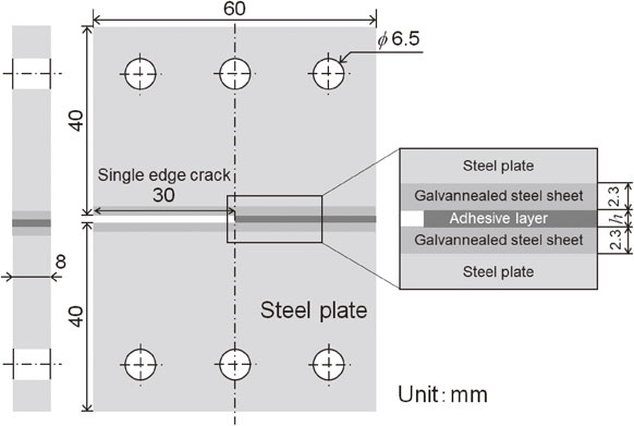
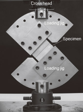
Figure 2 shows the appearance of the adhesive joint, fixed with an Arcan-type jig and attached to a tensile testing machine. The jig is connected to the testing machine with one pin at the top and bottom, and multiple pinholes are prepared so that the mounting angle of the specimen can be changed at a pitch of 15° around the center of the specimen. The arrangement in Fig. 2 corresponds to a state in which the bonding surface is inclined at 45° to the horizontal axis. It is expected that the condition of 0° with respect to the horizontal axis of the bonding surface corresponds to the so-called mode I, and 90° corresponds to mode II, and it is possible to perform a mixed-mode fracture test of the adhesive joint between these two angles.
2.2 Applicability of the Dugdale model
Figure 3 shows the result of the uniaxial tensile test of the automotive adhesive used in this paper. It is believed that the work hardening is small, and the adhesive is approximated as an elastic-perfect plastic material. Moreover, since steel is used as the adherent material in this paper, the plastic zone is limited to a narrow strip region in the adhesive layer. These conditions are in good agreement with the assumptions of the Dugdale model. Therefore, we consider a method to calculate the J-integral experimentally from the crack tip opening displacement of the adhesive end by extending the Dugdale model.
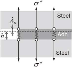
2.3 Mechanical model of the crack tip opening displacement and adhesive layer
Because the thickness of the adhesive layer is rather small compared to the specimen size, the specimen is assumed to be a single-edge notched specimen and fracture mechanics approach is applied. Figures 4, 5, and 6 show schematic illustrations of the adhesive end. The size of the opening in the vertical direction is λn, the size of the opening in the shear direction is λs, and the crack tip opening displacement λ is defined as
| \begin{equation}
\lambda = \sqrt{(\lambda_{n})^{2} + (\lambda_{s})^{2}}
\end{equation}
| (1) |
Next, with regard to the mechanical expression of the adhesive layer, the deformation of adhesive layer is assumed to be nearly uniform, because the displacement generated is limited to the thin adhesive layer. Then, as shown in
Figs. 4,
5, and
6, it is considered that the surface forces σ
* and τ
* in the vertical and shear directions respectively act on the adhesive surface. In addition, since there is local deformation at the adhesive end, as shown in the next section, simple correction parameters are introduced.
In the case when a pure mode I type opening deformation occurs in the adhesive layer (Fig. 4), or in the case of shear deformation of a pure mode II type occurs (Fig. 5), the crack tip opening displacement where yielding of the adhesive begins to occur is described as λnys and λsys. These can be expressed as eqs. (2) and (3).
| \begin{equation}
\lambda_{n}^{\text{ys}} = \frac{\sigma_{\text{ys}}}{E}h,
\end{equation}
| (2) |
| \begin{equation}
\lambda_{s}^{\text{ys}} = \frac{\tau_{\text{ys}}}{G}h,
\end{equation}
| (3) |
where σ
ys is the tensile yield stress of the adhesive, and τ
ys is the shear yield stress of the adhesive. In this study, it is assumed that
$\tau _{\text{ys}} = \sigma _{\text{ys}}/\sqrt{3} $.
E is the Young’s modulus of the adhesive,
G is the shear modulus of the adhesive, and
h is the thickness of the adhesive layer. From the true stress-true strain relationship shown in
Fig. 3, when the adhesive is considered as an elastic-perfect plastic material, σ
* and τ
* can be expressed with the magnitudes of λ
n and λ
s as
| \begin{equation}
\sigma^{*} =
\begin{cases}
\dfrac{\sigma_{\text{ys}}}{\lambda_{n}^{\text{ys}}}\lambda_{n} & \text{($0 \leq \lambda_{n} \leq \lambda_{n}^{\text{ys}}$)}\\
\sigma_{\text{ys}} & \text{($\lambda_{n}^{\text{ys}} \leq \lambda_{n}$)}
\end{cases}
,
\end{equation}
| (4) |
| \begin{equation}
\tau^{*} =
\begin{cases}
\dfrac{\tau_{\text{ys}}}{\lambda_{s}^{\text{ys}}}\lambda_{s} & \text{($0 \leq \lambda_{s} \leq \lambda_{s}^{\text{ys}}$)}\\
\tau_{\text{ys}} & \text{($\lambda_{s}^{\text{ys}} \leq \lambda_{s}$)}
\end{cases}
.
\end{equation}
| (5) |
Next, to consider the mixed-mode state of mode I and mode II (Fig. 6), the relative angle ξ between λn and λs is defined as in eq. (6). It was assumed that the crack tip opening displacement λys at the onset of yield under mixed mode can be determined using the linear rule of eq. (7) using ξ.
| \begin{equation}
\xi = \tan^{- 1}\left(\frac{\lambda_{s}}{\lambda_{n}}\right)
\end{equation}
| (6) |
| \begin{equation}
\lambda^{\text{ys}} = \lambda_{n}^{\text{ys}} + \frac{\lambda_{s}^{\text{ys}} - \lambda_{n}^{\text{ys}}}{\pi/2}\xi
\end{equation}
| (7) |
Generally, the Dugdale model treats post-yield stress conditions and implicitly assumes a mode I opening deformation. However, as shown in Fig. 3, in the case of the adhesive used in this study, the strain to yield is about 0.03, and the elastic range is never small. Therefore, we first try to evaluate the J-integral in the elastic region. Before the onset of the yielding, that is, 0 ≤ λ ≤ λys, it is represented by the sum of the elastic component $J_{\text{I}}^{\text{e}}$ for mode I of the J-integral and the elastic component $J_{\text{II}}^{\text{e}}$ for mode II, as shown in eq. (8). Here, mn, ms. $m_{n}^{\text{e}}$, and $m_{s}^{\text{e}}$ are the parameters for correcting the influence of stress concentrations and the influence of deformation constraints in the width direction and in the out-of-plane thickness direction.
| \begin{align}
J_{\text{CTOD}}^{\text{e}} & = J_{\text{I}}^{\text{e}} + J_{\text{II}}^{\text{e}} = m_{n} \int_{0}^{\lambda_{n}}\sigma^{*}d\lambda_{n} + m_{s} \int_{0}^{\lambda_{s}}\tau^{*}d\lambda_{s}\\
& = m_{n}^{\text{e}}\frac{\sigma_{\text{ys}}}{\lambda_{n}^{\text{ys}}}\lambda_{n}^{2} + m_{s}^{\text{e}}\frac{\tau_{\text{ys}}}{\lambda_{s}^{\text{ys}}}\lambda_{s}^{2}.
\end{align}
| (8) |
Further, even after the adhesive layer fully yields in the thickness direction, the Dugdale model is extended to consider both normal and shear stress components. After the onset of yielding, λys ≤ λ, so that the J-integral can be expressed as in eq. (9) using ξ.
| \begin{align}
J_{\text{CTOD}}^{\text{ep}} & = m_{n} \int_{0}^{\lambda^{\text{ys}}\cos \xi}\frac{\sigma_{\text{ys}}}{\lambda_{n}^{\text{ys}}}\lambda_{n}d\lambda_{n} + m_{s} \int_{0}^{\lambda^{\text{ys}}\sin \xi}\frac{\tau_{\text{ys}}}{\lambda_{s}^{\text{ys}}}\lambda_{s}d\lambda_{s}\\
&\quad + m_{n}^{p}\cos \xi \int_{\lambda^{\text{ys}}\cos \xi}^{\lambda_{n}}\sigma_{\text{ys}}d\lambda_{n} + m_{s}^{p}\sin \xi \int_{\lambda^{\text{ys}}\sin \xi}^{\lambda_{s}}\tau_{\text{ys}}d\lambda_{s}\\
& = m_{n}^{e}\frac{\sigma_{\text{ys}}}{\lambda_{n}^{\text{ys}}}(\lambda^{\text{ys}}\cos \xi)^{2} + m_{s}^{e}\frac{\tau_{\text{ys}}}{\lambda_{s}^{\text{ys}}}(\lambda^{\text{ys}}\sin \xi)^{2}\\
&\quad + m_{n}^{\text{p}}\sigma_{\text{ys}}(\lambda_{n} - \lambda^{\text{ys}}\cos \xi)\cos \xi \\
&\quad+ m_{s}^{\text{p}}\tau_{\text{ys}}(\lambda_{s} - \lambda^{\text{ys}}\sin \xi)\sin \xi.
\end{align}
| (9) |
In eqs. (8) and (9), if the elasto-plastic properties of the adhesive are known, the variables are only λn and λs. Here, $m_{n}^{\text{p}}$ and $m_{s}^{\text{p}}$ are parameters for correction of local deformation, that is, the effects of stress concentration and the effects of deformation constraints in the width direction and in the out-of-plane thickness direction, as in the above $m_{n}^{\text{e}}$ and $m_{s}^{\text{e}}$. If these four parameters are determined using finite element method analysis, etc., J-integral can be evaluated experimentally by measuring λn and λs. In the next section, simple formulas of eqs. (8) and (9) are verified by using finite element analysis.
3. Numerical Simulations
3.1 Numerical model
Numerical models are shown in Figs. 7–9. Each model has a load angle θ of 0°, 45°, and 90°. The adhesive layer, the plating layer (Zn layer), and the steel plate were modeled using plane-stress quadrilateral eight node elements. The thickness of the adhesive layer was changed as h = 0.3, 0.5, and 1.0 mm. The boundary conditions corresponding to the experiment were given for each model, and the analysis was conducted by changing the loading angles from 0° to 90°. The constitutive model of the adhesive is an elastic-perfect-plastic material, the rest are elastic materials, and the material constants are shown in Table 1. Note that ν is the Poisson’s ratio. Numerical simulations were carried out using Abaqus/Standard ver. 2018, a general-purpose finite element software.

Table 1 Material properties for FEM analysis.
The definition of the J-integral proposed by Rice19) is
| \begin{equation}
J_{\text{path}} = \int_{\varGamma}\left(Wdy - \sigma_{ij}n_{j}\frac{\partial u_{i}}{\partial x}ds \right),
\end{equation}
| (10) |
where
W is the strain energy density, σ
ij nj is the surface force vector,
ui is the displacement vector, and d
s is the increment of the length along the path
Γ. In recent general-purpose finite element softwares, the function for calculating the
J-integral based on this path integral formula (domain integral method
20)) is prepared as a standard function. The practical applicability of the simplified estimation formulas was evaluated by comparing the
J-integral, calculated using the simplified estimation formulas proposed in this paper, with the
J-integral obtained by numerical simulation. Here, for convenience, we denote the former as
JCTOD and the latter as
Jpath. While
Jpath originally assumes a continuous distribution of material constants, we set a wider integration region, as shown in
Fig. 7, in order to calculate across discontinuous adhesive layers. In addition,
JCTOD was calculated from the relative displacement of node A and node B corresponding to the crack front edge, as shown in
Fig. 7. The relative displacements in
x-
y coordinates are transferred to λ
n and λ
s, and
JCTOD is calculated using the simplified formulae of
eqs. (8) and
(9).
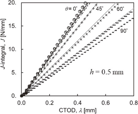
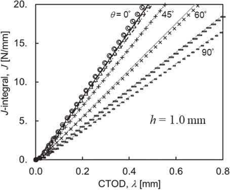
3.3 Numerical results
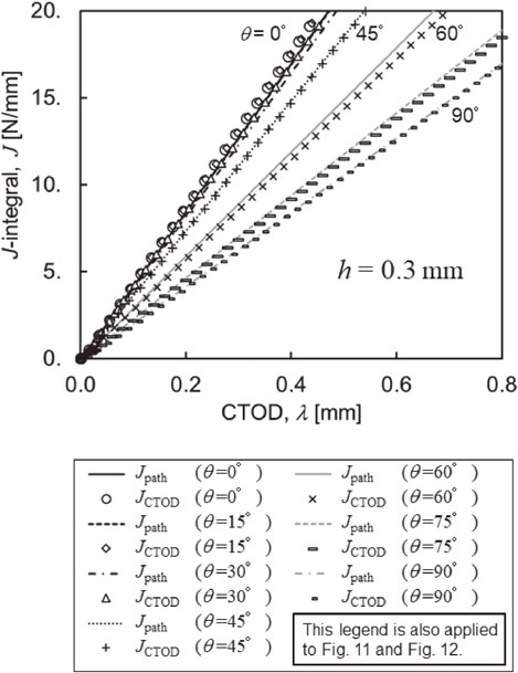
Numerical results for the adhesive layer thickness of h = 0.3, 0.5, and 1.0 mm are shown in Figs. 10–12, respectively. It is necessary to determine four parameters: $m_{n}^{\text{e}}$, $m_{s}^{\text{e}}$, $m_{n}^{\text{p}}$, and $m_{s}^{\text{p}}$. The coefficients related to the elastic region, $m_{n}^{\text{e}}$ and $m_{s}^{\text{e}}$, are determined by integrating eqs. (8) and (9), which results in $m_{n}^{\text{e}} = 1/\sqrt{3} $ and $m_{s}^{\text{e}} = 0.5$. As for the coefficients related to the plastic region, $m_{s}^{\text{p}}$ is assumed to be 1.0 as the Dugdale model uses plane stress and elastic-perfect-plastic material.21) $m_{n}^{\text{p}}$ is assumed to be 1.2, taking into account local deformation at the adhesive end. In the range studied in this paper, the results of Jpath, calculated based on numerical simulation, and JCTOD, calculated based on a simple evaluation formula, almost coincide with each other. Therefore, by using the simple evaluation formula proposed in the paper, the J-integral can be accurately obtained from CTOD, and the validity of the simple evaluation formula is shown. It is noted that there is no significant difference in the results, even if $m_{n}^{\text{p}} = 1.0$, where mode II is dominant, such as in the cases of θ = 75, 90°, although $m_{n}^{\text{p}}$ is effective in a region where θ is small. In addition, when the thickness of the adhesive layer is smaller, local deformation may concentrate more, and it may be necessary to make more than 1.2 corrections, especially for $m_{n}^{\text{p}}$.
4. Mixed-Mode Fracture Tests for GA Steel Adhesive Joints
GA steel sheets are subjected to galvanization heat treatment after galvanizing steel sheets for the purpose of corrosion protection. As a result, various Fe–Zn-based intermetallic compounds are formed at the interface between the steel and the plating layer.22) Therefore, several types of failure mode of adhesive joints can be considered, such as cohesive failure of the adhesive, interface failure of the adhesive and the adherent, fracture of the plating layer, and the mixture of these, which are related to the adhesive strength, loading angle, and adhesive thickness. In this section, the effects of adhesive thickness and loading angles on fracture toughness and failure mode are investigated.
4.1 Specimen
GA steel plates of 2.3 mm thickness were joined by laser welding to two SS400 steel plates 60 mm wide, 40 mm high, and 8 mm thick, as shown in Fig. 1. Teflon sheets, which have the same thickness as the adhesive layer (h = 0.3, 0.5, and 1.0 mm), were used as spacers, and two steel plates were bonded with a thermosetting epoxy resin over a width of 30 mm. After that, heat curing was carried out using an electric furnace.
4.2 Mixed-mode fracture tests
Figure 2 shows the apparatus for mixed-mode fracture tests. The specimens were fixed to a special jig, and the pin position between the jig and the tensile testing machine (Autograph AG-50kNX, Shimadzu) can be changed depending on the loading angle from 0° to 90° in 15° increments. Three experiments were carried out at each loading angle. In addition, fracture surfaces were observed under a microscope (VW6000, KEYENCE), and the ratio of the cohesive fractured surface to the adhesive layer was calculated using image processing software (Image J). In addition, the fractured surface was observed with a scanning electron microscope (TM3030 Plus, Hitachi High-Technologies), and energy dispersive X-ray (EDX) analyses were conducted, and the fracture location and fracture morphology were examined.
4.3 Measurements of CTOD by digital image correlation method
In order to accurately measure the crack tip opening displacement in mixed mode, non-contact measurement was performed using digital image correlation (DIC) software (VIC-2D ver. 2009, Correlated Solutions). Figure 14 shows a schematic view of the crack tip corresponding to Fig. 13. In DIC, the displacement components based on the global coordinate system of points A and B at the crack tip, $\delta _{x}^{A}$, $\delta _{y}^{A}$, $\delta _{x}^{B}$ and $\delta _{y}^{B}$, were measured. At the same time, to find out the angle of the specimen including the crack tip, the coordinate values at point 1, point 2, point 3, and point 4 were also obtained from DIC. Assuming that xi, yi (i = 1, 2, 3, 4) are coordinate values in x and y directions based on the entire coordinate system at point i, respectively, the average angle θsp is calculated using eq. (11). Then, the crack tip opening displacements, λn and λs, required to obtain the J-integral, can be calculated by eq. (12).
| \begin{equation}
\theta_{\text{sp}} = \frac{1}{2}\left\{\tan^{- 1}\left(\frac{y_{2} - y_{1}}{x_{2} - x_{1}} \right) + \tan^{- 1}\left(\frac{y_{4} - y_{3}}{x_{4} - x_{3}} \right) \right\}
\end{equation}
| (11) |
| \begin{equation}
\begin{pmatrix}
\lambda_{n}\\
\lambda_{s}
\end{pmatrix}
=
\begin{pmatrix}
\cos \theta_{\text{sp}} & \sin \theta_{\text{sp}}\\
-{\sin \theta}_{\text{sp}} & \cos \theta_{\text{sp}}
\end{pmatrix}
\left\{
\begin{pmatrix}
\delta_{x}^{\text{B}}\\
\delta_{y}^{B}
\end{pmatrix}
-
\begin{pmatrix}
\delta_{x}^{\text{A}}\\
\delta_{y}^{A}
\end{pmatrix}
\right\}
\end{equation}
| (12) |
5. Results and Discussion
5.1 Mixed-mode fracture tests
Figures 15, 16, and 17 show the relationship between the load and the crack tip opening displacement at each adhesive layer thickness and each loading angle (θ = 0, 30, 60, 90°). Note that λ is obtained from λn and λs by eq. (1). The cross-head displacement, measured by the tensile testing machine, included the looseness of the jig, and it was difficult to measure displacements precisely. However, by using DIC, it was possible to measure the process in which the crack tip opening displacement is almost stably changing with the load. At any thickness of the adhesion layer, the crack tip opening displacement up to the fracture was small under the condition that the loading angle was small, but ductile behavior was observed at θ = 90°, where shear deformation becomes dominant.


Figure 18 shows the relationship between fracture load and loading angle. Error bars indicate the range of maximum and minimum values. The fracture load is greater when the loading angle is larger and the adhesive layer is thinner. This is consistent with the empirical trend. Figure 19 shows the relationship between Jc and the loading angle. Jc was calculated using the simplified formulae of eqs. (8) and (9) by using the crack tip opening displacement λnc and λsc at the fracture. Almost constant Jc was obtained at 0° ≤ θ ≤ 60°, and no significant difference was observed for the adhesion layer thickness. It is believed that brittle fracture occurred in those cases due to local strain concentration. On the other hand, when 75° ≤ θ ≤ 90°, Jc clearly increases with increasing θ. It is considered that this is due to an increase of the plastic dissipation energy in the adhesive before fracture. At the same time, it was found that Jc tends to increase as the adhesive layer becomes thicker at 75° ≤ θ ≤ 90°, and the influence of plastic dissipation becomes larger. These tendencies agree with the tendencies of the crack tip opening displacements up to fracture, which were large when shear deformation becomes dominant in Figs. 15, 16, and 17.

Figure 20 shows the ratio of cohesive fracture to fracture surface. When the loading angle was small, the cohesive fracture of the adhesive was dominant, and when the loading angle became larger, the fracture of the plating layer became dominant. The fracture surface observed with a scanning electron microscope is shown in Fig. 21 for h = 0.3 mm and θ = 0°. In this case, the failure mode is cohesive fracture of the adhesive. Small voids of about several microns can be observed on the fracture surface, which is considered to be the origin of failure. Figure 22 shows the fracture surface for h = 0.3 mm and θ = 75°. In this case, the fractured surface was flat and showed a metallic luster. In addition, as a result of the EDX analysis, it can be seen that the Γ1 phase appears, and it is considered that fracture occurs at the interface between Γ1 phase and δ phase. Figure 23 shows the fracture surface for h = 0.5 mm and θ = 0°. In this case, the failure mode is a cohesive fracture of the adhesive, but there were not so many voids, such as h = 0.3 mm, and the evidence that the adhesive was stretched can be seen. Figure 24 shows the fracture surface for h = 0.5 mm and θ = 75°. Moreover, in this case, the fractured surface was flat and showed a metallic luster, but many surface cracks can be observed. As a result of the EDX analysis, Γ1 phase appears on the fracture surface, and it is believed that Γ1 phase or the interface between Γ1 phase and Γ phase was fractured. It is well known that Fe-rich Fe–Zn intermetallic compounds are brittle and cause peeling of the coating during press working.23) Therefore, when shear load is dominant, it is believed that the joint strength is determined not by the adhesive strength, but by the Fe–Zn intermetallic compound and its interface.

6. Conclusion
In this study, we proposed a simple J-integral evaluation formula for adhesive joints and applied it to mixed-mode fracture tests of adhesive joints using GA steel plates. As a result, the following findings were obtained:
-
(1)
Using the proposed simple evaluation formula, the J-integral in the mixed-mode state can be accurately obtained from the crack tip opening displacement.
-
(2)
Regarding fracture toughness, no significant relationship is observed between the adhesive layer thickness and Jc due to brittle fracture at 0° ≤ θ ≤ 60°. However, at 75° ≤ θ ≤ 90° due to the effect of plastic deformation in the adhesive layer, the larger the loading angle was, the greater the Jc. In addition, the effect of plastic dissipation strongly depends on the adhesive layer thickness.
-
(3)
Regarding the failure mode, cohesive fracture of the adhesive is dominant when the loading angle is small, but when the loading angle is large, the failure is dominant within the Fe–Zn intermetallic compounds. Therefore, it is considered that the joint strength of GA steel plates is determined not only by the adhesive strength, but also by the Fe–Zn-based intermetallic compound and its interface.
REFERENCES
- 1) C. Sato: JSAE Symposium, No. 07-17, (2017) pp. 19–22.
- 2) A.J. Kinloch: Adhesion and Adhesive: Science and Technology, (Chapman and Hall, London, 1987).
- 3) R.D. Adams ed.: Adhesive Bonding: Science, Technology, and Applications, (Woodhead Publishing Limited and CRC Press LCC, 2005).
- 4) ASTM D3433 – 99, “Standard Test Method for Fracture Strength in Cleavage of Adhesives in Bonded Metal Joints”, (2012).
- 5) B.R.K. Blackman, H. Hadavinia, A.J. Kinloch, M. Paraschi and J.G. Williams: Eng. Fract. Mech. 70 (2003) 233–248.
- 6) ASTM D7905/D7905M – 14, “Standard Test Method for Determination of the Mode II Interlaminar Fracture Toughness of Unidirectional Fiber-Reinforced Polymer Matrix Composites”, (2014).
- 7) Q.D. Yang, M.D. Thouless and S.M. Ward: Int. J. Solids Struct. 38 (2001) 3251–3262.
- 8) G. Fernlund and J.K. Spelt: Compos. Sci. Technol. 50 (1994) 441–449.
- 9) T.A. Hafiz, M.M. Abdel Wahab, A.D. Crocombe and P.A. Smith: Eng. Fract. Mech. 77 (2010) 3434–3445.
- 10) M. Omiya and K. Kishimoto: J. Soc. Mat. Sci., Japan 51 (2002) 1367–1372.
- 11) M. Omiya, K. Nakamura, R. Maeda, K. Ogawa, T. Kobayashi, T. Furusawa, E. Yokoi and K. Takada: Proceedings of the 65th JSMS Annual Meetings, (2016) pp. 97–98.
- 12) P. Jousset and M. Rachik: Eng. Fract. Mech. 132 (2014) 48–69.
- 13) I.S. Floros, K.I. Tserpes and T. Löbel: Compos., Part B 78 (2015) 459–468.
- 14) R.K. Joki, F. Grytten, B. Hayman and B.F. Sørensen: Compos. Sci. Technol. 128 (2016) 49–57.
- 15) D.S. Dugdale: J. Mech. Phys. Solids 8 (1960) 100–104.
- 16) G.I. Barenblatt: The Mathematical Theory of Equilibrium Cracks in Brittle Fracture, Advances in Applied Mechanics, Vol. 7, (Academic Press, New York, 1962) pp. 55–129.
- 17) B.A. Bilby, A.H. Cottrell and K.H. Swinden: Proc. R. Soc. London, Ser. A 272 (1963) 304–314.
- 18) T.L. Anderson: Fracture Mechanics Third Edition, (CRC Press, Boca Raton, 2005).
- 19) J.R. Rice: J. Appl. Mech. 35 (1968) 379–386.
- 20) Dassault Systèmes: SIMULIA User Assistance 2018, Abaqus, Analysis, (2018).
- 21) M. Shiratori, T. Miyoshi and H. Matsushita: Suuchi Hakai Rikigaku, (Jikkyo Shuppan, Tokyo, 1980) p. 18, 40.
- 22) S. Ochiai, T. Tomida, T. Nakamura, S. Iwamoto, H. Okuda, M. Tanaka and M. Hojo: Tetsu-to-Hagané 91 (2005) 320–326.
- 23) J. Inoue, S. Miwa and T. Koseki: Tetsu-to-Hagané 100 (2014) 53–59.