1. Introduction
1.1 Solidification of high-entropy alloys
High-entropy alloys (HEAs) have been studied for various properties, including the effect of their high entropy, the stability of their solid solution (FCC and BCC), and their mechanical properties and corrosion behavior.1–3) The CrMnFeCoNi system is a typical example of a high-entropy alloy.4) CrMnFeCoNi alloys solidify dendritically, forming a single FCC solid solution.
Based on scanning electron microscopy (SEM) with energy-dispersive spectroscopy (EDS), the HEAs have shown an interdendritic region that is poor in Fe and rich in Cr and Mn, indicating that solute partition occurs during solidification. CrMnFeCoNi alloys are simply described by a pseudo-binary CrFeCo–MnNi system.5) In this solidified structure, the core of the dendrite arms is rich in Co, Cr, and Fe, while the interdendritic region is rich in Mn and Ni.4) Previous reports4,5) have disagreed in these results, though, because multicomponent alloys exhibit a complicated equilibrium between liquid and solid phases. In addition, uncertainties remain in understanding the dendritic growth of HEAs, such as their preferred growth direction, dendrite arm spacing, and interfacial area. Thus, further study on the fundamental properties of dendritic growth in HEAs is required to quantitatively analyze their solidification.
In the present study, we aim to describe the three-dimensional structure of the growing dendrites, determine the preferred growth direction of the dendrite arms, and measure the solid–liquid interfacial area and average curvature in CrMnFeCoNi alloys by using X-ray imaging with synchrotron radiation. For comparison, the secondary dendrite arm spacing in the solidification structure was examined. By combining time-resolved tomography6) and X-ray diffraction (XRD),7) performed at the SPring-8 synchrotron radiation facility (Hyogo, Japan), the microstructure and crystallographic orientation were observed simultaneously.
1.2 Characterization of dendritic growth
Dendrite arms grow along a preferred crystallographic orientation, as well known. Grain selection during solidification, which determines the solidification structure, is influenced by the preferred growth direction. For example, changing the growth direction of the dendrite arms during solidification produces a casting defect called feathery grains.8) Thus, to understand solidification in the alloys of interest, the preferred growth directions should be measured.
When the kinetic undercooling at the solid–liquid interface is negligibly small, dendrites grow along a preferred crystallographic orientation. The preferred growth direction is determined by the anisotropy of the solid–liquid interfacial energy. The selection of the growth direction has been explained by considering the interface shape modified by anisotropy.9) The interface undercooling, ΔTr, owing to curvature is given by
| \begin{equation}
\Delta T_{r} = \left[ \frac{\gamma_{SL} + \gamma''_{SL}}{(\Delta S_{f}/v_{m})} \right]K
\end{equation}
| (1) |
Here, γ
SL,
$\gamma ''_{SL}$, Δ
Sf,
vm, and
K are the solid–liquid interfacial energy, the second derivative of the interfacial energy (orientation dependence), the entropy of fusion, the molar volume, and the curvature, respectively. As expressed in
eq. (1), the anisotropy of the interfacial energy produces a curved interface at equilibrium. Once the convex interface, where the curvature,
K, is maximum, grows faster, a dendrite arm develops in the preferred direction. However, such anisotropy is not understood systematically, even though understanding anisotropy would improve our understanding of morphological evolution. Thus, measuring the preferred growth direction of the dendrites should give some insights on the anisotropy.
The preferred growth direction of typical FCC crystals (such as Al, Cu, Ni, and γ-Fe) is ⟨100⟩.10) The reported directions10) of FCC and BCC crystals suggest that the anisotropy of the solid–liquid interface is induced by the FCC and BCC structures themselves, promoting the ⟨100⟩ directional growth.
The solid–liquid interfacial energy could be modified by adding solutes and by changing the growth conditions if the anisotropy is weak.11,12) The difference in the solid–liquid interfacial energy is as small as 2% for the Al–4 mass% Cu alloy.13) In Al–Zn alloys, the growth direction of the dendrite continuously changes from ⟨100⟩ to ⟨110⟩ in the {110} plane as the Zn content increases from 5 mass% to 90 mass%.14–17) In addition, based on CT and EBSD, the seaweed-like dendrites were far from random, and their growth direction was still constrained within the {100} plane symmetry.16,17) To the best of our knowledge, though, the preferred growth directions of dendrites in HEAs have not been identified systematically.
1.3 Observation methods
In the last twenty years, in-situ observation techniques using synchrotron radiation X-rays have been developed extensively in third-generation synchrotron radiation facilities. At first, the solidification of metallic alloys with relatively low melting points—such as Sn-, Al-, and Mg-based alloys—were observed in situ by 2D transmission imaging.18–22) Later, this technique was extended to observe solidification in Cu-, Ni-, and Fe-based alloys at temperatures above 1300 K.23–27) Such 2D imaging techniques can observe microstructure evolution during solidification, but cannot quantitatively measure the preferred growth orientation, solid–liquid interfacial area, or curvature of the solid–liquid interface.
Time-resolved tomography (3D plus time, referred to as 4D-CT) can be used to observe the 3D microstructure evolution in metallic alloys. Using this technique, Ludwig et al.28) observed the microstructure of Al–4 mass% Cu alloys (X-ray: pink beam, diameter: 1 mm, cooling rate: −0.1 K/s, rotation: 0.1 rps). 4D-CT has also been used to observe melting and solidification in Al–Mg–Si–Y2O3 alloys,28) and to observe coarsening of dendrite arms in Al–Cu alloys.29) Time-interlaced model-based iterative reconstruction (TIMBIR), which improves temporal resolution, has been used to observe solidification in Al–15 mass% Cu alloys.29) 4D-CT has also been used to demonstrate semi-solid deformation and transgranular liquation cracking in Al–Cu alloys.30–32)
A filtering technique using a phase field model, which improves image quality even at relatively high temporal resolution, has been proposed to evaluate the solid–liquid interfacial area and the average curvature in a Fe–0.45 mass% C–0.6 mass% Mn–2 mass% Si alloy at high temperatures above 1700 K.6) This filtering removed voxel-scale noise and improved the evaluation, allowing 4D-CT to be extended to Fe- and Ni-based alloys with relatively large X-ray absorption coefficients. In addition, XRD has been performed using a 4D-CT setup,7) obtaining the distribution of crystallographic orientations over time by measuring XRD spots on a 2D detector. Thus, in the present study, we combine 4D-CT and XRD to simultaneously observe the evolution of microstructure and crystallographic orientation.
2. Experimental Procedure
Equimolar CrMnFeCoNi alloys were made from Cr (99.9%), Mn (99.9%), Fe (99.99%), Co (99.9%), and Ni (99%) in an arc-melting furnace. Specimens for 4D-CT (0.8 mm in diameter and 5 mm in length) and for thermal analysis (3.7 mm × 3.7 mm × 0.85 mm, ∼90 mg) were obtained from the as-cast buttons.
4D-CT and XRD were performed at the BL20XU imaging beamline of the SPring-8 synchrotron radiation facility (Hyogo, Japan). The X-rays, generated by an undulator light source, were monochromatized using a Si (111) double-crystal monochromator. An X-ray energy of 37.7 keV was selected. A four-jaw slit was used to form the incident beam size. The typical beam size was 5 mm in width and 2 mm in height.
Figure 1 shows the setup for the 4D-CT and XRD measurements. A coordinate system with x–y–z axes are defined in Fig. 1(a). The 4D-CT setup was basically the same as that used in a previous study,6) as was the XRD setup.7) A sample on a rotating stage, a panel-type detector for the XRD images, and a beam monitor for the transmission images were placed along the X-ray beam, as shown in Fig. 1(a). The distance between the sample and the panel-type detector was ∼0.3 m, and the distance between the sample and the beam monitor was ∼0.5 m. The panel-type detector with a pixel size of 100 µm × 100 µm and a pixel matrix of 992 × 672 was used to take XRD images at a frame rate of 30 fps. The beam monitor with a pixel size of 6.5 µm × 6.5 µm took transmission images at a frame rate of 100 fps. The pixel matrix was set to be 850 (width) × 300 (height) to adjust the specimen size. The specimen was rotated at 0.25 rps (360° rotation took 4 s). A stepping motor controller, which controlled the rotation, also generated trigger signals to take transmission and XRD images at every rotation step of 0.9° and 3.0°, respectively.

The specimen in the high-purity alumina pipe (0.8 mm in inner diameter, 2 mm in outer diameter) was placed in a carbon furnace. The rotating specimen was melted and then cooled at a cooling rate of 0.083 K/s in a vacuum atmosphere (∼10−1 to 100 Pa). The temperature gradient at the specimen was serval K/mm. Projected images (transmission images) and XRD images were continuously recorded during cooling.
Convolution back projection (CBP) image reconstruction was performed using 200 projection images over a 180° rotation. To reduce noise in the reconstructed images, the raw reconstructed images were normalized using the images of the liquid phase just before solidification, the normalized images were processed using a Gaussian filter (smoothing/blur filter), and then the smoothed images were used as initial conditions for a filter using a phase field model (referred to as a PF filter).7) Before the PF filter, the solid fraction at every time step was estimated from the distribution of the X-ray absorption coefficient in the smoothed images. This procedure is explained briefly in the next section, and the detailed procedure is described in a previous work.7)
As shown in Fig. 1(b), a diffraction spot position on the panel-type detector and a rotation angle, ω, give the normal vector of the diffraction plane determined by the diffraction angle, 2θ. The setup for XRD was the same as that for three-dimensional XRD microscopy (3DXRD).33,34) Although the beam size of 2 mm in height degraded the spatial resolution in 3DXRD, the diffraction spots still gave the position of the diffracting grain. As shown in Fig. 1(b), the diffraction position was used to confirm the grain position in the specimen.
Specimens solidified a constant cooling rate (0.0033, 0.083, 0.17, 0.33, and 0.67 K/s) were prepared with a differential scanning calorimetry apparatus. The local solidification time was estimated from the cooling curve. The solidification structure was assessed by mapping Mn in SEM/EDS images, and the secondary arm spacing was measured from these Mn maps.
3. Results and Discussion
3.1 Reconstruction of growing dendrites
Figure 2(a) show a snapshot of the transmission image. The transmission intensity at the center of specimen was approximately a tenth smaller than that outside the specimen and crucible. Figure 2(b) shows an example of the projection images used for the reconstruction. The transmission images reflected the microstructure, even though the transmission intensity was low.

Figure 3(a) shows a reconstructed image (slice image) with no image processing. Although dendrite arms appear, it is difficult to track the solid–liquid interface smoothly and to reproduce the 3D dendritic structure. As shown in Fig. 3(b), intense noise remains in the image normalized by the liquid image before solidification. However, the normalization did reduce the gradual change of intensity in the a–b direction. As shown in Fig. 3(c), a Gaussian filter reduced the noise with a relatively short wavelength, although the solid–liquid interface blurred. Even with the Gaussian filter, though, it was still difficult to track the solid–liquid interface.

Using the images with the Gaussian filter, we evaluated the solid fraction as a function of time, as shown in Fig. 4. The distribution of intensities in the reconstructed images, which are proportional to the linear X-ray absorption coefficient, was fitted by two different Gaussian functions: one is the liquid phase and the other is the solid phase. The solid fraction was used as a constraint condition in the PF filter.6)
Here, we will briefly explain PF filtering.6) The average curvature, K, is defined by
| \begin{equation}
\frac{1}{K} = \frac{1}{K_{1}} + \frac{1}{K_{2}}
\end{equation}
| (2) |
where
K1 and
K2 are the principal curvature. When the solid grains of a pure substance are isolated in the liquid phase in isothermal conditions, the average curvature should be the same at any solid–liquid interface point in equilibrium. For alloy dendrites in isothermal conditions, the presence of a non-uniform distribution of solutes could change the average curvature distribution. However, the solute concentration difference in the interdendritic liquid region (10–100 µm) is relatively small. Thus, we propose that the solid–liquid interface was modified so that the average curvature at every interface point was equal.
Because the curvature effect is inherently included in phase field models,35–38) filtering using a phase field model was proposed.6) First, the 3D images with the Gaussian filter were converted into a phase field, ϕ, by eq. (3):
| \begin{equation}
\phi =
\begin{array}{cl}
0 & (I > I_{\textit{Liquid}})\\
\frac{I - I_{\textit{Liquid}}}{I_{\textit{Solid}} - I_{\textit{Liquid}}} & (I_{\textit{Liquid}} > I > I_{\textit{Solid}})\\
1 & (I_{\textit{Solid}} > I)
\end{array}
\end{equation}
| (3) |
Here,
I is the brightness of the reconstructed images, and
ILiquid and
ISolid are the threshold parameters to identify the liquid and the solid phases, respectively.
Second, the phase field was calculated using eqs. (4a)–(4c):
| \begin{align}
\Delta \phi&= -(M\Delta t)\Big[ -6\phi (1-\phi) \frac{\sigma}{r} \\
&\quad + 2\phi (1 - \phi) (1 - 2\phi)W - \varepsilon^{2}\nabla^{2}\phi \Big]
\end{align}
| (4a) |
| \begin{equation}
W = \frac{3\sqrt{2}\sigma}{\delta}
\end{equation}
| (4b) |
| \begin{equation}
\varepsilon^{2} = 3\sqrt{2}\sigma \delta
\end{equation}
| (4c) |
Here, (
MΔ
t) is a parameter of the time step. Notably, this parameter does not influence the calculated results if the parameter is sufficiently small.
W is another parameter that includes the interfacial energy, σ, and interfacial thickness, δ. The interfacial energy was set to be 0.2 J/m
2, and the thickness was two or four times as large as the voxel size of the phase field. This parameter mainly stabilizes the thickness of interface in the phase filed and has only a minor influence on the filtering result if an appropriate value is given. ε
2 is a parameter depending on the interfacial energy, σ, and the thickness, δ. This parameter also has a minor influence, although the iteration number in FP filter depends on the value. In the filtering, a critical parameter is the radius,
r, defined in
eq. (4a). The radius is a driving force for motion of the solid–liquid interface. If an invalid value is given, the solid fraction calculating from the phase field deviates from the value obtained from the reconstruction images.
Given these parameters, the phase field was sequentially calculated by eqs. (4a)–(4c). If the given parameters are appropriate, the solid fraction calculated from the phase field converges to the solid fraction evaluated from the reconstructed images after Gaussian filter. In the PF filter, the appropriate parameter r as a function of time must be explored. As shown in Fig. 3(d), the dendrite arms were clearly reconstructed by the PF filter with the appropriate parameters. Figure 4 shows the solid fraction as a function of solidification time, which was calculated from the phase field. The solid fractions obtained by the reconstructed images and the PF filter agree with each other and follow the square-root law, which is commonly observed in specimens solidified at a constant cooling rate.
Figure 5 shows 3D reconstructed images of the growing dendrites during cooling. Even at the initial stage of solidification, where the solid fraction was less than 0.1, the primary and the secondary dendrite arms appeared in the 3D images, and two dendritic grains appeared. A fragmented dendrite grain, which is a seed of grain 1, moved down from the top due to buoyancy and was stacked. Grain 2 continuously grew from the bottom. In general, the primary and the secondary dendrite arms are developed at the early stage of solidification and then the dendrite meets another dendrite. Namely, the coherent dendrite network is formed. The solid fraction at which this takes place, is defined as the dendrite coherency point fraction. As shown in Fig. 5(b), the coherent dendrite network was developed entirely in the observation region at a solid fraction between 0.1 and 0.2. As shown in Fig. 5(c), the dendrite arms coarsened after the dendrite coherency point. The dendrite coherency point fraction depends on the alloy composition and grain morphology,39) varying from less than 0.1 (for poorly refined Al alloys) to more than 0.5 (for fine-grained Al alloys). Because the two coarse grains grew in the observation, the dendrite coherency point fraction observed in the present study is consistent with a previous study.39)
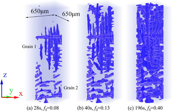
Figure 6(a)–(c) shows XRD images obtained by the panel-type detector during the solidification time of 660–664 s. As shown in Fig. 6(a), a rectangular (111) spot appeared, 1 mm in width and 1.5 mm in height. This spot indicates that the diffraction grain size is nearly 1 mm in width and more than 1 mm in height. Similar rectangular shapes appeared for (200), (220), and (311) diffraction spots. According to the 3D reconstructed images shown in Fig. 5, two dendritic grains appeared in the observation region. The rectangular shapes are consistently explained by the 3D reconstructed images.

Figure 6(d) shows an XRD image obtained by integrating the diffraction images over a 360° rotation. Enough diffraction spots were detected to determine the crystallographic orientations of the grains. As mentioned in the previous section, the XRD setup was the same as that for 3DXRD,33,34) except that the X-ray beam size was larger in the present study. Thus, the positions of the diffraction spots were used to confirm the positions of the diffracting grains. For example, the (220) spot indicated by “L” had a lower diffraction angle than the (220) spot indicated by “U.” Grains 1 and 2 shown in Fig. 5 produced the diffraction spots “U” and “L,” respectively, shown in Fig. 6.
Figure 7(a) shows the intensities of the diffraction spots in a stereo projection. The diffraction spots of (111), (200), (220) and (311) are plotted on the same projection. The gray arrow between the two dashed lines shows the measurable region of the XRD spot in the present setup. Figure 7(b) shows the crystallographic orientations of grains 1 and 2. All of the diffraction spots measured by the panel-type detector were used for this analysis. The setting matrix defined by
| \begin{equation}
\begin{bmatrix}
x\\
y\\
z
\end{bmatrix}
= \mathrm{M}
\begin{bmatrix}
h\\
k\\
l
\end{bmatrix}
\end{equation}
| (5) |
where M is the setting matrix. The matrices of grains 1 and 2 were obtained as follows.
| \begin{equation*}
\begin{bmatrix}
-0.96 & 0.26 & 0.03\\
0.01 & -0.06 & 1.00\\
0.26 & 0.96 & 0.06
\end{bmatrix}
,\
\begin{bmatrix}
-0.24 & 0.19 & 0.95\\
0.73 & -0.62 & 0.30\\
0.64 & 0.77 & 0.01
\end{bmatrix}
.
\end{equation*}
|
The preferred growth direction was determined by combining the 3D reconstructed images and the crystallographic orientations. Figure 8 shows close-up views of grain 1 with the crystallographic orientation on a stereo projection. In Fig. 8(a), the dendrite arms indicated by “R” are perpendicular to the printing surface. The growth direction of the arms is defined as $\boldsymbol{{r}} = ( - 0.01,0.01,1.00)$ in the x–y–z coordinate system. The directions $\boldsymbol{{p}} = (0.97, - 0.24,0.01)$ and $\boldsymbol{{q}} = (0.24,0.95, - 0.01)$ are also parallel to the dendrite arms indicated by “P” and “Q,” respectively. As shown in Fig. 8(c), the directions p, q, and r coincide with the ⟨100⟩ directions of grain 1. The directions $\boldsymbol{{s}} = (0.96, - 0.28,0.00)$, $\boldsymbol{{t}} = ( - 0.03, - 0.12, - 0.99)$, and $\boldsymbol{{u}} = ( - 0.27, - 0.95, - 0.12)$ in Fig. 8(b), which are parallel to the dendrite arms, also coincide with the ⟨100⟩ directions in Fig. 8(c).

Figures 8(d) and (e) shows the 3D reconstructed images and crystallographic orientation of grain 2. The directions $\boldsymbol{{p'}} = (0.69,0.72,0.02)$, $\boldsymbol{{q'}} = ( - 0.26,0.24,0.93)$ and $\boldsymbol{{r'}} = (0.67, - 0.65,0.35)$ are parallel to the dendrite arms. The directions $\boldsymbol{{s'}} = (0.66,0.75,0.02)$, $\boldsymbol{{t'}} = (0.72, - 0.60,0.36)$ and $\boldsymbol{{u'}} = (0.28, - 0.22, - 0.93)$ are also parallel to the dendrite arms. As shown in Fig. 8(f), all the directions coincide with the ⟨100⟩ directions of grain 2. Thus, the preferred growth direction of the dendrites in the CrMnFeCoNi alloy is the ⟨100⟩ directions, which is typical in FCC alloys.10)
The anisotropy of the solid–liquid interfacial energy changes the growth direction from ⟨100⟩ to ⟨110⟩ as the Zn content increases in Al–Zn alloys.14–17) If the five constituent elements are randomly distributed in the FCC structure and in the melt, a random configuration—defined as a type of entropy effect—may reduce the anisotropy arising from atomic bonding. This can reduce the anisotropy of the solid–liquid interfacial energy arising from the bonding. If this assumption is valid, we can attribute the preferred ⟨100⟩ growth direction of the CrMnFeCoNi alloy to the FCC structure itself. Also, the fact that the preferred growth direction of ⟨100⟩ for pure substances with an FCC structure10) seems to agree with this assumption. Further studies from various viewpoints are required to discuss how the inherent structure affects the preferred growth direction. The finding of the present study is that the dendritic growth and the grain selection during solidification in CrMnFeCoNi alloys can be analyzed using solidification models developed for conventional FCC alloys with a ⟨100⟩ preferred growth direction.
3.4 Characterization of the solid–liquid interface
The solid–liquid interfacial area and the average curvature were evaluated from the 3D reconstructed images after the PF filter. Figure 9 shows the specific interfacial area, SV—which is defined as the normalized interfacial area divided by the total volume (solid and liquid phases)—as a function of solid fraction. The interfacial area shows a maximum at a solid fraction of 0.55 and the maximum value was 2.5 × 10⁴ m−1.
The specific interfacial area, AV, which is defined as the normalized interfacial area divided by the solid volume, was estimated to be 14 × 104 m−1 at a solid fraction of 0.2 in an Al–24 mass% Cu alloy solidified at 0.033 K/s.40) The value of AV is converted to be 2.8 × 10⁴ m−1 in SV. In addition, the specific interfacial area, SV, was ∼2.5 × 10⁴ m−1 at a solid fraction of 0.5 in a Mg–15 mass% Sn alloy solidified at 0.2 K/s.41) Thus, the specific interfacial area in the CrMnFeCoNi alloy is on the same order as those in Al–Cu and Mg–Sn alloys.
Figure 9 shows the average curvature as a function of solid fraction ranging from 0.08 to 0.8. The average curvature decreases with increasing solid fraction and becomes zero at a solid fraction of 0.6. The curvature, K, is defined by
| \begin{equation}
K = \frac{dS}{dV_{S}} = \frac{dS_{V}}{df_{S}}
\end{equation}
| (6) |
where
S and
VS are the solid–liquid interfacial area and the solid volume, respectively. Thus, if the average curvature is uniform in the specimen, the solid fraction where the specific interfacial area is maximum (0.55) should match the solid fraction where the average curvature is zero (0.6). However, these two solid fractions are different as shown in
Fig. 9. This difference has two possible reasons: measurement inaccuracy or a non-uniform distribution of average curvature in the dendritic structure.
In addition to the inconsistent in the solid fractions, the solid–liquid interfacial area was not maximum at a solid fraction of 0.5. The dendrite arms with trunk shape are developed at lower solid fractions while the liquid phase tends to be spheroidal droplets isolated by the solid phase. Thus, the solid shape at the low solid fractions quite differs from the liquid shape at the high solid fractions. The asymmetric morphologies can shift the solid fraction where the interfacial area is maximum. For example, the interfacial area in Al–10 mass% Cu alloy at 0.05 K/s was maximum around at a solid fraction of 0.55.42) In a phase field simulation,43) the interfacial area was maximum around at 0.6. These results42,43) suggest that the interfacial area as a function of solid fraction is asymmetric about the solid fraction of 0.5. It should be noted that there are still limited reports on the interfacial area. Further studies are needed to understand the solid-fraction dependence of the interfacial area systematically.
3.5 Secondary dendrite arm spacing
Figure 10 shows the microstructures solidified at cooling rates of 0.033–0.67 K/s. Microsegregation caused by the dendritic growth appeared in the Mn maps from SEM/EDS. Figure 11 shows the secondary dendrite arm spacing, evaluated from the microstructure, and the relationship between the local solidification time and cooling rate. The secondary arm spacing of 40 µm, which was measured from the 3D reconstructed images at a solid fraction of 0.1, is marked in this figure with a red rectangle. This spacing of 40 µm at a low solid fraction is less than half of the spacing observed in the solidification structure. Thus, more than half of the secondary arms disappeared during coarsening.
The relationship between the secondary dendrite arm spacing and the local solidification time is given by10)
| \begin{equation}
\lambda_{\textit{II}} \propto \left[ \frac{\Gamma D_{L}}{m (1-k) C_{0}}t_{f} \right]^{1/3}
\end{equation}
| (7) |
where Γ and
DL are the Gibbs–Thomson coefficient and diffusivity in the liquid phase, respectively.
m,
k, and
C0 are the slope of the liquidus line, the solute partition coefficient, and the average solute concentration, respectively. The secondary arm spacing measured in the present study qualitatively agrees with
eq. (7).
The secondary arm spacings, 40–150 µm, are within the typical range found in metallic alloys. According to eq. (7), the spacing depends on the solid–liquid interfacial energy and diffusivity in the liquid phase. Sluggish diffusion in the solid phase has been noted in CrMnFeCoNi alloys.44,45) If the diffusivity in the liquid phase is measurably lower, the spacing should be smaller. Thus, our results suggest that the physical properties of CrMnFeCoNi alloys, such as their Gibbs–Thomson coefficient and solute diffusivities in the liquid phase, are typical for metallic alloys. Notably, the solidification in CrMnFeCoNi alloys can be discussed using conventional solidification models. However, the solidification path in such alloys should be investigated quantitatively. Critically, our understanding of solidification in HEAs will be improved by measuring the solute partitions at the solidifying front and by simplifying the multi-component solidification for quantitative analysis.


