Development of a Numerical Simulator for 3-D Dynamic Fracture Process Analysis of Rocks Based on Hybrid FEM-DEM Using Extrinsic Cohesive Zone Model

Abstract

The combined finite-discrete element method (FDEM) is one of the promising hybrid methods that has attracted much interest for the numerical simulations of complex fracture processes of rocks. The mainstream FDEM simulators developed to date are based on the intrinsic cohesive zone model (ICZM) in which cohesive elements are inserted into all the boundaries of continuum solid elements at the onset of simulations, and a penalty elastic behavior must be incorporated to model the intact deformation of rocks. However, previous studies have not systematically discussed the effect of the introduction of the penalty elastic behavior on the precision of intact stress wave propagation, and this paper discusses this concern. This paper applies an FDEM based on the extrinsic cohesive zone model (ECZM) as an alternative to the FDEM(ICZM). An advantage of the FDEM(ECZM) is first presented through a three-dimensional (3D) numerical modeling of a dynamic tension test. In addition, the effect of considering the anisotropy of wave propagation in granite, which has been neglected in all the previous works using the FDEM, is investigated through the 3D FDEM(ECZM) simulation of a dynamic Brazilian test using a split-Hopkinson pressure bar apparatus. Through the presented numerical simulations, we can conclude that the FDEM(ECZM) is a useful alternative to FDEM(ICZM) for numerical simulations of complex dynamic fracture processes of rocks.

 

This Paper was Originally Published in Japanese in J. Soc. Mater. Sci., Japan 69 (2020) 228–235.

1. Introduction

Various computational methods have been proposed for reasonably accurate analyses of the dynamic fracturing of rocks.¹⁾ However, no method is the best because each computational method has its own characteristics. The application of the hybrid method, which incorporates the advantages of each method to overcome their disadvantages, has attracted much interest.¹⁾ The combined finite-discrete element method (FDEM) was proposed by Munjiza²⁾ as one of the promising hybrid methods, and it has been applied to analyses of the dynamic fracturing of rocks.^3–6) In the framework of the explicit finite element method (FEM), the FDEM can model (i) “continuous deformation processes”, (ii) “transition from continuum to discontinuum (initiation of microcracks, their propagation and formation of macro fracture)”, and (iii) “very complex contact interactions between material surfaces including those of newly formed macro fractures”. The items (i)–(iii) are modeled by “continuum deformation of solid elements,” “relative opening and sliding of initially zero-thickness cohesive elements inserted between the solid elements,” and “potential-based contact force theory,”²⁾ respectively. For example, several previous studies^3–6) applied the two-dimensional (2D) and three-dimensional (3D) FDEM to model the dynamic Brazilian tensile strength (BTS) test based on the split-Hopkinson pressure bar (SHPB) apparatus. These studies indicated that FDEM is applicable to modeling resultant fracture patterns and the strain-rate dependency of the BTS. However, the majority of FDEM codes, including those in the above studies, have been implemented based on the intrinsic cohesive zone model (ICZM).⁷⁾ As explained later, introducing the penalty behavior of initially-zero thickness cohesive elements is indispensable with the ICZM. Accordingly, a compromise in the precision of simulated stress wave propagation in intact rocks may occur. However, no previous study related to FDEM has systematically discussed this concern. Furthermore, in terms of the stress wave propagation, granite has been known to have an anisotropy of strength according to the ease of opening along the “rift”, “grain”, and “hardway”. The first and second weakest planes are the rift and grain, respectively. The hardway is perpendicular to both the rift and grain.⁸⁾ Generally, intact granite exhibits significant anisotropy in its wave velocity. However, although previous studies modeled granite using the FDEM, the velocity anisotropy was not considered.

This study investigated the application of 3D FDEM based on an extrinsic cohesive zone model (ECZM)⁷⁾ as an alternative to the FDEM(ICZM). The simulation results of a dynamic tension test of a rock using 3D FDEM(ICZM) and FDEM(ECZM) were compared. Subsequently, a 3D FDEM(ECZM) simulation of an SHPB-based dynamic BTS test considering the anisotropy of wave velocity in the intact granite was conducted.

2. Overview of 3D FDEM

This section briefly reviews only the important aspects of 3D FDEM as the full details of the fundamental theory of the FDEM(ICZM) simulator used in this study are provided in the literature,^9,10) and the FDEM(ICZM) and FDEM(ECZM) are similar except for the treatment of the initially zero-thickness cohesive elements. Unless either the ICZM or ECZM is specified, the treatment between the FDEM(ICZM) and FDEM(ECZM) is exactly the same in the following explanation.

In 3D FDEM, the stress wave propagation of intact rocks due to dynamic loading is modeled using the dynamic elastic deformation of 4-noded tetrahedral elements (TET4s) (Fig. 1).¹⁰⁾ The input parameters for each TET4 are the elasticity tensor and mass density.

Fig. 1

Schematic illustration of a CE6 connecting two TET4s by normal and shear cohesive tractions (σ^coh, τ^coh).

The initiation and propagation of microcracks in a 3D FDEM are modeled by the relative opening and sliding of the initially zero-thickness 6-noded cohesive elements (CE6s), which are inserted between TET4s corresponding to a rock model (Fig. 1). For the constitutive behavior of the CE6s, a combined single and smeared crack concept based on the cohesive zone model (CZM)¹¹⁾ is used. In this approach, depending on the amount of the relative opening, closing, or sliding of the CE6s, the cohesive tractions, σ^coh and τ^coh, acting normal and parallel to the two surfaces of the CE6s, respectively, are computed. Terms σ^coh and τ^coh are determined based on the tensile and shear softening laws in which the Mohr-Coulomb shear strength model with tension-cutoff is utilized.¹⁰⁾ The mixed mode I-II crack growth characterized by the simultaneous crack opening and sliding is also considered according to the literature.¹⁰⁾ Because σ^coh and τ^coh exhibit a significant spatial gradient in a CE6, the 7-point Gaussian integration scheme is used for the conversion of σ^coh and τ^coh to the equivalent nodal force. CE6s can be inserted by considering the ICZM and ECZM.⁷⁾ The difference between the ICZM and ECZM is explained using the tensile softening model in a CE6 as an example (Fig. 2). In Fig. 2, the horizontal axis “o” (positive value: opening) indicates the amount of relative opening between the two faces of the CE6, i.e., the opening of microcracks. The vertical axis indicates the normal cohesive traction σ^coh (positive value: tension). σ^coh is applied to the two faces of the CE6 in a manner that it prevents the CE6 from opening. For the ICZM, CE6s are inserted between all the boundaries of TET4s at the onset of the simulation. Therefore, the penalty elastic behavior corresponding to the region 0 ≦ o ≦ o_p is indispensable; otherwise, the stress propagation in the intact rocks cannot be modeled at all. The term o_p is given as o_p = 2hT_s/P_coh, in which h, T_s, and P_coh are minimum edge length, microscopic tensile strength, and cohesive penalty of the CE6, respectively.^9–11) Because the CE6 based on the CZM is originally introduced only to model the post-peak regime characterized by the material softening, the condition of P_coh → ∞ (i.e., o_p → 0) is required.¹¹⁾ However, the critical timestep, Δt, requires to be infinitesimal to ensure the stability of the simulation under P_coh → ∞. Because the FDEM is based on the explicit FEM, this is impossible. Therefore, a finite value must be used for P_coh, and the bulk wave velocity of the rocks simulated from the ICZM-based method is always expected to become generally smaller than that theoretically estimated from elasticity tensor and mass density assigned to the TET4s. As a compromise, in the previous studies using the FDEM(ICZM),^3,12) P_coh was set to, for example, 1–10 times the value of Young’s modulus used for solid elements (3-noded triangle elements in 2D; TET4s in 3D). However, this approach of setting P_coh was seemingly proposed primarily for the application to problems under quasi-static loading, while the effect of P_coh on the stress wave propagation in the intact rocks, which is the essential function in rock dynamic problems, was not extensively discussed. This aspect is discussed in Section 3.

Fig. 2

Difference between (a) ICZM and (b) ECZM in the scenario of opening mode in a CE6.

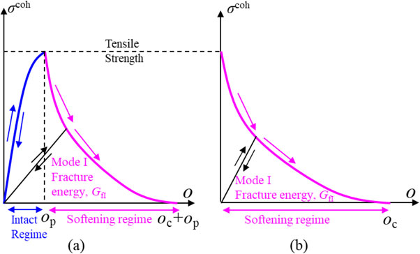
In contrast, the ECZM does not insert the CE6s at the onset of the simulation. Instead, by monitoring the normal and shear stresses acting on each boundary of the TET4s, a CE6 is adaptively inserted to the corresponding boundary when either normal stress or shear stress attains the given microscopic strength to the boundary. Here, a cumbersome modification of the element-node connectivity is required. This study adopted the adaptive remeshing algorithm originally proposed for the insertion of 12-noded cohesive elements between 10-noded tetrahedral elements,¹³⁾ and the algorithm was modified to enable the CE6s to be adaptively inserted between TET4s. Different node splitting techniques were used depending on the location of the CE6 insertion. In each scenario, the nodes to be split were located within the rock mesh (Fig. 3(a)), on a surface of the rock mesh (Fig. 3(b)) and on an edge of the rock mesh (Fig. 3(c)). The scenario shown in Fig. 3(d) corresponded to the special scenario of Fig. 3(c), in which all the three nodes to be split were on different edges of the rock mesh. With the remeshing algorithm in the ECZM, considering the penalty elastic behavior as in the ICZM (Fig. 2(a)) was no longer necessary, and the CE6 in the ECZM could only model the material softening (Fig. 2(b)). In this scenario, the 3D FDEM(ECZM) before the insertion of the CE6s was equivalent to the pure explicit FEM, which can consider large displacement and rotation using only continuum solid elements (TET4s).¹⁰⁾ Thus, the precision of the stress wave propagation in intact rocks using the FDEM(ECZM) is better than using the FDEM(ICZM). The common input parameters for a CE6 both in the ICZM and ECZM are the microscopic tensile strength, cohesion, and internal friction angle along with mode I and II fracture energies. Generally, experimentally evaluating these microscopic parameters is difficult; thus, the calibration procedure by Tatone et al.¹²⁾ was applied to determine these parameters in a manner that the bulk or macroscopic behavior of rocks observed in the experiment could be captured adequately. In the FDEM(ICZM), P_coh must be additionally specified. The stress wave propagation under P_coh → ∞ in the ICZM must converge to that in the ECZM, i.e., pure dynamic FEM. Therefore, the precision in the stress wave propagation of the intact rocks obtained by the ECZM should generally be higher than the ICZM.

Fig. 3

Adaptive remeshing scheme using the node splitting technique implemented for 3D FDEM(ECZM).

To model very complex contact mechanics between solid surfaces including newly formed macroscopic fractures (i.e., the faces of broken CE6s), the 3D FDEM uses the potential-based penalty method proposed by Munjiza²⁾ to compute repulsive and frictional forces due to contact. With this method, one of the two contacting discrete bodies is called a “contactor” while the other is called a “target”. In typical 3D FDEM, the contactor and target are subdivided into multiple TET4s. Subsequently, the computation of the contact force between the overlapping contactor and target is resolved into those between TET4s included in the contactor and target. When a TET4 in the contactor (contactor TET4) and a TET4 in the target (target TET4) are overlapped, the exact shape and area of the contact plane are evaluated. Subsequently, the contact repulsive force proportional to the contact area is computed and applied normal to the contact surface with the proportional factor, P_DEM. In addition, the contact friction between the contactor and target TET4s is modeled based on Coulomb’s friction law.^9,10) For an efficient contact detection algorithm, the non-binary-search algorithm²⁾ is used, and it exhibits the computational complexity O(N), with N being the number of TET4s subjected to the contact detection. For contact calculation, the input parameters are P_DEM and the friction coefficient.

After computing the equivalent nodal forces corresponding to the above modeling aspects of the 3D FDEM, the nodal accelerations, velocities, and positions were explicitly updated using the central difference scheme.^9,10) The selection of stable time step Δt must satisfy the Courant condition at least, which results in a very small Δt. The 3D FDEM(ICZM) and FDEM(ECZM) were implemented using the Fortran programming language based on a sequential computation.

3. Comparison between FDEM(ICZM) and FDEM(ECZM)

This section describes the analysis of the dynamic fracture process of a dynamic tension test of a rock conducted using the 3D FDEM(ICZM) and FDEM(ECZM), and the differences between the obtained results are discussed.

3.1 Overview of dynamic tension test and numerical model

The dynamic tension test of a rock using a single Hopkinson pressure bar was set as the target problem, which used a longer rock specimen than those used in the dynamic BTS and dynamic compression tests.¹⁴⁾ In the test, the spalling phenomenon due to the Hopkinson effect¹⁵⁾ was used and the stress wave propagation in the intact rocks had a more important function than other dynamic tests in terms of the numerical modeling. The test was called a “spalling test” for simplicity. A Geochang granite obtained from Korea was used. In the spalling test conducted in this study (Fig. 4), a metal projectile called a striker bar was accelerated using a gas gun, and the striker was hit to one end of a long cylindrical metal bar called an incident bar (IB). Subsequently, an approximately one-dimensional (1D) compressive stress wave, σ_inci, propagated toward the other end of the IB on which the cylindrical rock specimen (diameter = 38 mm, length = 180 mm) was set. At the interface between the IB and the rock specimen, a portion of the σ_inci was reflected as a tensile stress wave, σ_refl, while the remaining portion was transmitted into the rock specimen as a compressive stress wave, σ_trans. When the σ_trans reached the free end of the rock specimen, the σ_trans was reflected as a tensile stress wave and propagated back to the IB side. Due to this tensile stress, one or more macroscopic fracture planes that were approximately normal to the axial direction of the rock specimen were formed by the spalling phenomena at a certain distance from the free end. Figure 4 shows the spalling process observed using high-speed imaging (HSI). While two macroscopic fracture planes were observed in the resultant rock fracture pattern, the formation of the left macroscopic fracture was only observed during the HIS observation, which indicated that the right one formed after the left one. The left macroscopic fracture plane was defined as the “first observed macro fracture”. In addition, the free surface particle velocity (FSPV) at the free end of the rock specimen (x = 180 mm in Fig. 4) was also monitored using a laser displacement sensor (see also Fig. 7(a) explained later). The results of the 3D FDEM(ICZM) and FDEM(ECZM) were compared in terms of these experimental proofs.

Fig. 4

Overview of spalling test including high-speed camera images and a photo of fractured specimen.

Figure 5 shows the 3D FDEM model for the spalling test. Although the FDEM can model the detailed contact process,²⁾ a significant amount of computation is required.^9,10) Because the main aim of this study was the comparison of the ICZM and ECZM, the striker bar and IB were not explicitly modeled to reduce the computational amount. Thus, we considered that the 1D theory of stress wave propagation across the different elastic media was useful for modeling the contact between the IB and rock specimen in the spalling test. In this scenario, the ratio of σ_inci in the IB to σ_trans in the rock specimen can be given as follows:¹⁵⁾   

\begin{equation} \frac{\sigma_{\text{trans}}}{\sigma_{\text{inci}}} = \frac{2\rho_{1}C_{1}A_{1}}{\rho_{0}C_{0}A_{0} + \rho_{1}C_{1}A_{1}} \end{equation} (1)

where A₀, ρ₀, and C₀ are the cross-sectional area, mass density, and longitudinal wave velocity of the IB, respectively; and A₁, ρ₁, and C₁ are those of the rock specimen. In this experiment, the value of the left-hand side of eq. (1) was 0.4. In addition, σ_inci in the IB was obtained from the strain wave profile measured on the strain gauge attached on the IB (Fig. 4) multiplied by the Young’s modulus of the IB. Subsequently, the profile of σ_trans in the rock specimen with respect to time, t, was evaluated using 0.4 × σ_inci, according to eq. (1). The pressure function, P(t), which was equivalent to the profile of σ_trans, was applied to the one end of the numerical rock model (x = 0) (Fig. 5). Following this procedure can approximately model the contact interaction between the IB and rock specimen. We did not consider the anisotropy of the target granite to focus only on the difference between the ICZM and ECZM. Thus, the granite in the intact regime was assumed to behave as a homogeneous isotropic elastic body. Considering the laboratory tests, Young’s modulus (E), Poisson’s ratio (ν), and mass density (ρ) of the granite were set to 40.6 GPa, 0.2, and 2641.0 kg/m³, respectively. Based on the mechanical properties of the granite under quasi-static loading and the calibration procedure by Tatone et al.,¹²⁾ the microscopic tensile strength, cohesion, and internal friction angle of the granite were set to 15.0 MPa, 36.7 MPa, and 50°, respectively. Both the mode I and II fracture energies of the rock were assumed to be 400 J/m². Because P_coh must be set in the ICZM, P_coh = 1E, 5E, 10E, and 50E were simulated considering the previous studies.^{3–6,9–12)} Δt = 10 ns was used for all the FDEM simulations. With this value of Δt, the FDEM(ECZM) exhibited no numerical instability while the ICZM could operate without instability as long as P_coh ≦ 50E. Thus, a Δt less than 10 ns was required if the FDEM(ICZM) simulation with such as P_coh = 100E and 200E were to be conducted.

Fig. 5

Numerical model and boundary condition for 3D FDEM simulation of the dynamic spalling test.

3.2 Results

To indicate the difference between the ICZM and ECZM, Fig. 6 shows the propagation of σ_xx (cold color: compression; warm color: tension) along the x direction at t = 20 µs, in which only the region near the pressurized face (x = 0) is displayed. All the scenarios indicated that the wavefront of the compressive stress wave traveled a certain distance from x = 0. With the ECZM, no CE6 was inserted and this result was similar to the elastodynamic FEM simulation with E = 40.6 GPa and ν = 0.2 having the highest precision among all the scenarios. In contrast, the result of the ICZM(P_coh = 1E) exhibited a traveling distance of the stress wave that was approximately 50% shorter than with ECZM, i.e., the P-wave velocity was significantly underestimated. This was evidentially caused by the very small P_coh with a significant effect of the penalty elastic behavior (0 ≦ o ≦ o_p in Fig. 2(a)) on the increase of the bulk compliance of the rock. Moreover, the stress distribution in the ICZM(P_coh = 1E) was significantly noisy compared with the ECZM. With a larger P_coh in the ICZM, the bulk wave velocity became comparable to the ECZM with less noise in the stress distribution. However, even the ICZM(P_coh = 50E) exhibited a slightly slower P-wave velocity than the ECZM. Thus, a larger P_coh with a smaller Δt must be used considering that the stable simulation of the FDEM(ICZM) with Δt = 10 ns could only be ensured for P_coh ≦ 50E. This resulted in a further increase in computational time in the ICZM. Because the 3D FDEM simulation required a large amount of computation,¹⁰⁾ the FDEM(ECZM) was seemingly superior in terms of computational time and the precision of modeling stress waves in intact rocks.

Fig. 6

Comparison of intact stress wave propagation obtained by 3D FDEM based on ICZM and ECZM at t = 20 µs.

Figures 7(a) and (b) show the profiles of the FSPV and resultant fracture patterns obtained from the experiment and 3D FDEM simulations. In Fig. 7(b), the fracture planes enclosed by the red ovals were the first observed macro fracture planes defined above, which were determined by the HSI and FDEM simulations. These results indicated that the ECZM simulation could adequately capture the profile of the FSPV, fracture pattern, and position of the first observed macro fracture. The ICZM(P_coh = 1E) indicated that the arrival of the stress wave, identified by the time of the commencement of the FSPV rising in Fig. 7(a), was significantly delayed than in other scenarios. Moreover, the peak value of the FSPV and location of the first observed macro fracture were completely different from the experiment. Considering the results shown in Figs. 6 (i.e., noisy and slower stress wave propagation) and 7 (i.e., higher peak value of the FSPV), the results of the FDEM(ICZM) with P_coh = 5E∼10E were far from satisfactory compared with the experiment and FDEM(ECZM). However, the ICZM (P_coh = 50E) exhibited a similar result to the experiment and ECZM.

Fig. 7

Comparison between the experimental results and those obtained from 3D FDEM based on ICZM and ECZM.

4. 3D FDEM(ECZM) Considering the Anisotropy of Granite

This section discusses the investigation on the effect of the anisotropy of granite on the FDEM result, which was neglected in previous studies.^3–6) Only the 3D FDEM(ECZM) was used because of the superiority in modeling the stress wave propagation of intact rocks, and the granite was modeled as an orthotropic elastic body. This required proper setting of the elasticity tensor in the constitutive equation for the TET4s, and the new self-consistent scheme (NSCS)¹⁶⁾ was adopted. The NSCS modeled the orthotropic elasticity of the granite considering the distribution of pre-existing microcracks.¹⁷⁾ We considered that the orientations of the microcracks in the granite could be categorized into two mutually orthogonal groups in addition to a group with random orientation. By successively adding penny-shaped microcracks into an intact elastic body, the effective elasticity tensor for the granite was computed by integrating the change of bulk stiffness.¹⁶⁾ In addition to modeling the anisotropy of the elasticity tensor, 3D FDEM(ECZM) may also consider the anisotropy of the microscopic strength. However, previous studies indicated that dynamic fracture toughness of granite exhibited significantly minor anisotropy in the scenarios of high loading rate.¹⁸⁾ Hence, more experimental evidence must be accumulated to model and investigate the strength anisotropy. Thus, only the orthotropic elasticity was considered in the 3D FDEM(ECZM) simulation described below.

4.1 Overview of SHPB-based dynamic BTS test and numerical model

The previously reported SHPB-based dynamic BTS test of Barre granite³⁾ was simulated using 3D FDEM(ECZM). Similar to the spalling test, this test used the gas gun and striker to generate the stress wave in the IB. The SHPB also used a transmission bar (TB) in addition to the IB to dynamically load the rock disc.^3,14)

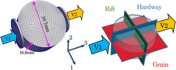
Figure 8 shows the 3D numerical model for the SHPB-based dynamic BTS test of the Barre granite. Generally, the anisotropy of granite becomes less apparent when pre-existing cracks are closed under high hydrostatic pressure. If all pre-existing cracks are closed, the anisotropy disappears.¹⁶⁾ Based on this evidence, the effective elasticity tensor of Barre granite was computed using NSCS in which the above-described three groups of microcracks were successively added to the elastic body with E = 80 GPa and ν = 0.25.¹⁶⁾ Hereafter, the directions perpendicular to the hardway, grain, and rift planes were simply called axes 1, 2, and 3, respectively. The measured P-wave velocities in intact Barre granite along axes 1–3 were 4.63, 3.94, and 3.67 km/s, respectively.¹⁹⁾ Table 1 shows the effective elasticity tensor obtained from the NSCS.

Fig. 8

Numerical model for SHPB-based dynamic Brazilian test.

Table 1 Effective elasticity tensor estimated for Barre granite.

Following Mahabadi et al.,³⁾ the rigid thin disc models were used to model the portions of the IB and TB near the rock specimen and experimentally evaluated velocities V₁(t) and V₂(t) (see Fig. 8(a) in the Ref. 3)) were applied to the IB and TB, respectively. Considering the experimental condition, the dynamic loading direction using the IB and TB was set along axis 3 of the orthotropic elastic rock model (Fig. 8). This simulation is termed “BD-Ani” in the following discussion. For comparison, another simulation considering the isotropic body (this scenario is termed “BD-Iso”) was also conducted by assuming that v = 0.16³⁾ and the value of E was set in a manner that the theoretical P-wave velocity in the isotropic model matched with that along axis 3. Except for the elasticity tensor, all the other input parameters for the BD-Ani and BD-Iso were the same as in the previous study.³⁾

4.2 Results

Figures 9 and 10 show the time-history of the dynamic indirect tensile stress and resultant fracture pattern, respectively, for BD-Ani and BD-Iso. In addition, Fig. 9 shows the experimental result.³⁾ In Fig. 10, the resultant fracture pattern is depicted using the simulation result 58 µs after the attainment of the peak shown in Fig. 9. For BD-Ani, Table 1 implies that the rock model rendered the highest and lowest rigidities along axes 3 and 1, respectively. Because the elasticity tensor for BD-Iso was set in a manner such that the P-wave velocity became the same as that along axis 3 in BD-Ani, the stiffnesses along axis 3 both in BD-Ani and BD-Iso were the same while the BD-Iso along axes 1 and 2 rendered lower stiffnesses than those in BD-Ani.

Fig. 9

Time-history of dynamic indirect tensile stress. Note that the experimental data is obtained from Fig. 9 in Ref. 3).

Fig. 10

Resultant fracture patterns on the surface.

Figure 9 indicates that the peak value of the indirect tensile stress (i.e., dynamic BTS) in BD-Iso was slightly higher than that in BD-Ani although both scenarios exhibited good agreement with the experiment. The comparison of the resultant fracture patterns for BD-Ani and BD-Iso in Fig. 10 indicates significantly minor differences in terms of the central splitting fracture and crushed zone formed near the IB and TB. Additionally, BD-Iso depicts the generation of the macroscopic fractures enclosed by the dotted ovals, which were not observed in BD-Ani. However, because this type of macroscopic fracture is sometimes observed in the dynamic BTS,³⁾ the fracture patterns of the BD-Iso may be reasonable. To discuss the cause of the difference in the dynamic BTS between the two simulations, Fig. 11 shows the spatial distribution of the Cauchy stress tensor, σ₁₁, on the clipped plane, which passed through the center of the rock model and was perpendicular to axis 2. The result corresponded to t = 68 µs and no CE6 had been inserted at this moment, i.e., the regime was intact. Term σ₁₁ in both simulations exhibited qualitatively the same tendency while the BD-Ani exhibited a locally higher tensile stress value than BD-Iso in the central region. With this difference, a more local initiation and propagation of microcracks could be expected in the BD-Ani, resulting in the reduction of the dynamic BTS of the bulk rock. However, we may conclude that the detailed consideration of the orthotropic elasticity in granite resulted in minimal differences compared with the isotropic elasticity model in terms of the time-history of the dynamic indirect tensile stress and resultant fracture pattern in the target rock size. This indicated that the proper calibration of the isotropic elasticity tensor may still achieve satisfactory results.

Fig. 11

Spatial distributions of σ₁₁ on the clipped plane.

5. Discussion

Based on the above results, this section discusses the advantages and disadvantages of the FDEM(ICZM) and FDEM(ECZM). As mentioned above, the primary stream of previous studies developing and applying the FDEM applied the 2D or 3D FDEM(ICZM).^{2–6,9–12)} However, as shown in Section 3, the value of P_coh for the CE6s must be sufficiently large; otherwise, the precision of the stress wave propagation in the intact rocks is significantly compromised. Meanwhile, a larger P_coh increases the generation of the high-frequency noise that may trigger the instability of the FDEM simulation.¹⁰⁾ Therefore, in addition to the application of artificial damping to suppress the high-frequency noises, a relatively smaller value of Δt should be used in the FDEM(ICZM) compared with the Δt satisfying the Courant condition in the ordinary explicit FEM. These characteristics of the FDEM(ICZM) should also apply to such as the coupled FEM-DEM¹⁾ in which the processes (i)–(iii) mentioned in Section 1 are modeled by introducing elastic springs between the deformable elastic zones from the onset of the simulation. However, the results in this study clearly indicate that the reduction in P_coh in the FDEM(ICZM) or elastic springs in the coupled FEM-DEM must be avoided if the purpose is to use a larger Δt to shorten the simulation time. Otherwise, the velocity and precision of the stress wave propagation in the intact rocks exhibit a significant deviation from the theoretical behavior expected from the input elastic parameters. Thus, when either the FDEM(ICZM) or coupled FEM-DEM is applied to analyses of the dynamic fracture processes of rocks, the detailed calibration of the stress wave propagation in the intact rocks is indispensable, while the previous studies^3,6) did not show such results.

In contrast, the CE6 in the FDEM(ECZM) can only address the material softening (Fig. 2(b)), and the use of the penalty elastic behavior in the CE6 can be avoided. Thus, the precision of the FDEM(ECZM) in the intact deformation regime before the insertion of the CE6s is exactly the same as for the dynamic FEM, which is the most important concern in this paper. In the analysis of the dynamic fracture process, the stress wave propagation in the intact regime is the most important phase as the initiation and propagation of the microcracks are caused by the stress wave. In the CZM, the CE6 is originally intended to model the post-peak regime, and the penalty elastic behavior in the ICZM must not affect the bulk elastic behavior.¹⁰⁾ Thus, the CE6 must be distinguished from the joint element that is used to model physical discontinuity such as joints and faults in the rocks. For example, if a rock model consists of CE6s with an improperly set P_coh and joint elements, the CE6 part can decrease the accuracy of the simulation and adversely affect the behavior of joint elements, whereas the ECZM does not suffer from these challenges.

However, the ECZM has significant disadvantages. An example is that the parallel computation of the remeshing algorithm is extremely cumbersome, which makes analyzing the dynamic fracture process of significantly larger scale rock masses using the FDEM(ECZM) challenging. In this sense, the implementation of the parallel computation into the FDEM(ICZM) is much easier.^9,10) Therefore, the authors consider that the FDEM(ICZM) is still useful as long as a sufficiently large P_coh is applied and numerical instability is carefully monitored.

6. Conclusion

The development and application of the 3D FDEM(ECZM) were investigated. The FDEM(ECZM) was shown as able to simulate the stress wave propagation in intact rocks with a higher precision than the FDEM(ICZM), which has been the mainstream tool in the FDEM community. The drawbacks of the FDEM(ICZM) are clarified in the paper. In particular, for the same Δt, the precision of the stress wave propagation in intact rocks in the FDEM(ICZM) is compromised because of the penalty elastic behavior of CE6s controlled by P_coh; thus, a Δt smaller than that of the FDEM(ECZM) must be used for a higher precision. Therefore, the FDEM(ECZM) was suggested to have the advantage in terms of modeling “continuous deformation considering larger displacement and rotation,” “initiation and propagation of microcracks,” and “contact interaction between material surfaces” with higher precision.

Using the advantage of the ECZM, the analysis of dynamic fracture processes considering the orthotropic elasticity of the granite was conducted. The obtained results exhibited good agreement with a previous study.³⁾ Through a comparison of the scenarios of isotropic and anisotropic wave velocity, the obtained results exhibited some differences including resultant fracture pattern. However, as this study did not model the anisotropy of the microscopic strength because of lack of experimental evidence, our future task includes conducting dynamic tests for granite to accumulate more data of dynamic strength and fracture toughness along the principal directions of the stress wave propagation.

REFERENCES

• 1)   M.  Mohammadnejad,  H.  Liu,  A.  Chan,  S.  Dehkhoda and  D.  Fukuda: Geosys. Eng. (2018) 1–24.
• 2)  A. Munjiza: The Combined Finite-discrete Element Method, (John Wiley & Sons, Hoboken, 2004).
• 3)   O.K.  Mahabadi,  B.E.  Cottrell and  G.  Grasselli: Rock Mech. Rock Eng. 43 (2010) 707–716.
• 4)   D.  Osthus,  H.C.  Godinez,  E.  Rougier and  G.  Srinivasan: Int. J. Rock Mech. Min. Sci. 106 (2018) 278–288.
• 5)   H.C.  Godinez Vazquez,  E.  Rougier,  D.A.  Osthus,  Z.  Lei,  E.E.  Knight and  G.  Srinivasan: Int. J. Numer. Anal. Methods Geomech. 43 (2019) 30–44.
• 6)   E.  Rougier,  E.E.  Knight,  S.T.  Broome,  A.J.  Sussman and  A.  Munjiza: Int. J. Rock Mech. Min. Sci. 70 (2014) 101–108.
• 7)   Z.  Zhang,  G.  Paulino and  W.  Celes: Int. J. Numer. Methods Eng. 72 (2007) 893–923.
• 8)   Y.  Nara,  H.  Kato,  T.  Yoneda and  K.  Kaneko: Int. J. Rock Mech. Min. Sci. 48 (2011) 316–335.
• 9)   D.  Fukuda,  M.  Mohammadnejad,  H.Y.  Liu,  S.  Dehkhoda,  A.  Chan,  S.H.  Cho,  G.J.  Min,  H.  Han,  J.  Kodama and  Y.  Fujii: Int. J. Numer. Anal. Methods Geomech. 43 (2019) 1797–1824.
• 10)   D.  Fukuda,  M.  Mohammadnejad,  H.Y.  Liu,  Q.B.  Zhang,  J.  Zhao,  S.  Dehkhoda,  A.  Chan,  J.  Kodama and  Y.  Fujii: Rock Mech. Rock Eng. 53 (2020) 1079–1112.
• 11)   A.  Munjiza,  K.R.F.  Andrews and  J.K.  White: Int. J. Numer. Methods Eng. 44 (1999) 41–57.
• 12)   B.S.A.  Tatone and  G.  Grasselli: Int. J. Rock Mech. Min. Sci. 75 (2015) 56–72.
• 13)   A.  Pandolfi and  M.  Ortiz: Eng. Comput. 18 (2002) 148–159.
• 14)   Q.B.  Zhang and  J.  Zhao: Int. J. Rock Mech. Min. Sci. 60 (2013) 423–439.
• 15)  Z.X. Zhang: Rock Fracture and Blasting Theory and Applications, (Butterworth-Heinemann, Oxford, 2016).
• 16)   Y.  Nara and  K.  Kaneko: Int. J. Rock Mech. Min. Sci. 43 (2006) 437–453.
• 17)   O.  Sano: J. Soc. Mater. Sci. 37 (1988) 159–165 (Japanese manuscript with English abstract/figure captions/table captions).
• 18)   F.  Dai and  K.W.  Xia: Int. J. Rock Mech. Min. Sci. 60 (2013) 57–65.
• 19)   M.J.  Iqbal and  B.  Mohanty: Rock Mech. Rock Eng. 40 (2007) 453–475.