Damage Model Determination for Predicting Creep Rupture Time of 2 1/4Cr–1Mo Steel Weld Joints

Abstract

In a creep damage analysis for a weld joint (WJ) using a damage model, it is important to select a damage model that properly reflects complex conditions of stress generated in the interface between the base metal and the heat-affected zone (HAZ). For 2 1/4Cr–1Mo steel, we examined what type of scalar stress is appropriate to properly reflects the conditions of stress generated around the HAZ for accurately predicting creep rupture time, in the framework of the time exhaustion rule, which evaluates damage as a function of stress. For a specimen of a round rod WJ through which an HAZ penetrates obliquely, we compared actual tests and finite element method (FEM) analysis, in temperature-stress ranges from 120 to 160 MPa at 823 K, and from 80 to 100 MPa at 873 K. Using FEM calculations, we evaluated the rupture time based on the time exhaustion rule, considering three types of scalar stress: the maximum principal stress, the equivalent stress, and the Huddleston stress. Comparing with the tests, we found that the scalar stress that gives an appropriate rupture time is the Huddleston stress. In this stress, the damage accumulation due to the creep deformation in the base metal (BM)-HAZ interface and the cavity formation due to the hydrostatic pressure are taken into account. Analyses of the stress distribution inside and outside of the HAZ and in the BM-HAZ interface indicated that, for the 2 1/4Cr–1Mo steel, the cavity formation due to the tensile hydrostatic pressure is also important when we evaluate damage. We optimized a parameter b, which regulates the balance in the Huddleston stress, so that the observed results are reproduced with the determination coefficient of R² = 0.948, and we obtained the value of b as b = 0.34.

(a) Distributions of three principle stresses σ₁, σ₂, and σ₃, equivalent stress σ_eq, and Huddleston stress σ_Hud along the central axis of the FEM model; (b) Prediction performance of the time exhaustion rule model using Huddleston stress with the optimized parameter of b = 0.34.

1. Introduction

It is known that WJs of heat-resistant steel, such as 2 1/4Cr–1Mo steel, ruptures due to Type IV fracture of the fine-grained heat-affected zone (HAZ) where grain refining occurs.^1–3) Creep tests using a simulated HAZ specimen where the thermal history during the welding time was reproduced showed that the rupture time of the simulated HAZ where grain refining occurs becomes significantly shorter than the rupture time of the base metal (BM).^1,4,5) However, it is known that the rupture time of the WJ is longer than the rupture time of the simulated HAZ, and the rupture time ratio adopts the following order: the simulation HAZ < the WJ < the BM.^6,7) Intuitively, we can understand that this is because the HAZ is sandwiched between the BM and the weld metal (WM), and the creep deformation is constrained. In contrast, it is considered that, in addition to the creep deformation, the cavity formation at a high temperature under tensile stress also has an influence on the creep damage, and it is not necessarily obvious whether constraining deformation can suppress damage or not. Both the constraint of the creep deformation and the cavity formation under stress are strongly influenced by the multiaxiality generated in the HAZ. Hence, to quantitatively predict the rupture time of a WJ, it is necessary to evaluate a stress tensor during a creep test, combining models of creep deformation and damage.

To solve this numerically, it is effective to perform calculation using the finite element method (FEM). That is, we can calculate time evolutions of creep deformation and damage in the HAZ and its vicinity, based on constitutive equations of creep deformation and creep damage. What we need to focus on is how creep damage is related to stress. In particular, we need to appropriately treat the three-dimensionality of stress, in other words, multiaxiality.

The creep damage accumulated on a material is a scalar quantity itself, and it is necessary to have a framework that connects a stress tensor, which represents the multiaxiality of stress, and the creep damage, which is a scalar. The time exhaustion rule (TER) is known as the simplest framework for this, in which damage is expressed as a function of scalar stress.⁸⁾ In this framework, we evaluate a stress tensor by converting to a scalar stress. There have been several examinations of determining an appropriate scalar stress to express damage accumulation.^9–11) Huddleston⁹⁾ examined SUS304 and proposed the Huddleston stress, which is a modification of the equivalent stress, by taking the hydrostatic pressure component into account. In addition, Watanabe et al.¹⁰⁾ examined the damage distribution in a WJ creep specimen using Gr.91 steel, and they pointed out that the damage accumulation distribution in the welded part with Type IV fracture is consistent with the distribution of the Huddleston stress in an FEM model that simulates the shape of the HAZ in the specimen. Moreover, Koiwa et al.¹¹⁾ performed an FEM analysis of a WJ using several damage models that includes the TER for Gr.91 steel; they reported that, within the framework of TER, the scalar stress that best reproduces the rupture time of actual WJ is the equivalent stress. The most appropriate stress to make a prediction of the rupture time of WJ varies depending on the material and test conditions.

In this study, we focus on 2 1/4Cr–1Mo low alloy steels which are used in large-diameter steam piping in power stations. The establishment of a technology to predict the rupture time of a WJ, which is indispensable to manufacture piping, will enable us to optimize the welding process conditions numerically. In the materials integration project of the Cabinet Office SIP, optimization of the welding conditions is addressed.¹²⁾ Aiming at the establishment of a technology to predict the rupture time of a WJ made from the abovementioned material, we investigate to what extent we can make a prediction under the framework of the TER. In particular, under the TER, we examine the scalar stress that is appropriate to make an accurate prediction of the rupture time of a WJ. Performing actual creep tests for the BM and simulated HAZ, we determined creep parameters. We also performed creep tests for a WJ. Making an FEM model that simulates the WJ specimen, we performed a damage calculation by means of the FEM. Considering the obtained result, we examined the scalar stress that is appropriate for a damage calculation in the framework of the TER. Furthermore, we discussed the stress distribution around the HAZ, and we examined the value of the parameter b for the Huddleston stress.

2. Materials and Method

2.1 Target material, creep rupture test, and FEM analysis method

For 2 1/4Cr–1Mo steel, we prepared round rod specimens of the BM, a simulated HAZ, and a WJ, using the following procedures, and we performed creep tests with a constant load at a constant temperature.

Table 1 shows the composition of sample materials of the base material, the simulated HAZ, and the WJ. The sample material is ASME SA387M Grade 22 Class 2, which is a standard steel for 2 1/4Cr–1Mo steel. For the simulated HAZ, to simulate grain refining of prior austenite grains due to the heat affection during the welding time, as a reproduction heat treatment, we increased the temperature in a vacuum atmosphere at a rate of 50 K/s, up to 1198 K, held the temperature for 15 s, cooled at a rate of 15 K/s down to 673 K using Argon gas flows. In addition, we performed post-weld heat treatment (PWHT) (993 K–0 K, +10 K; 2 h–0 h, +0.2 h).

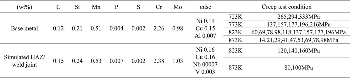
Table 1 Chemical composition for specimens, creep test conditions for base metal, HAZ, and weld joint of 2 1/4Cr–1Mo steel.

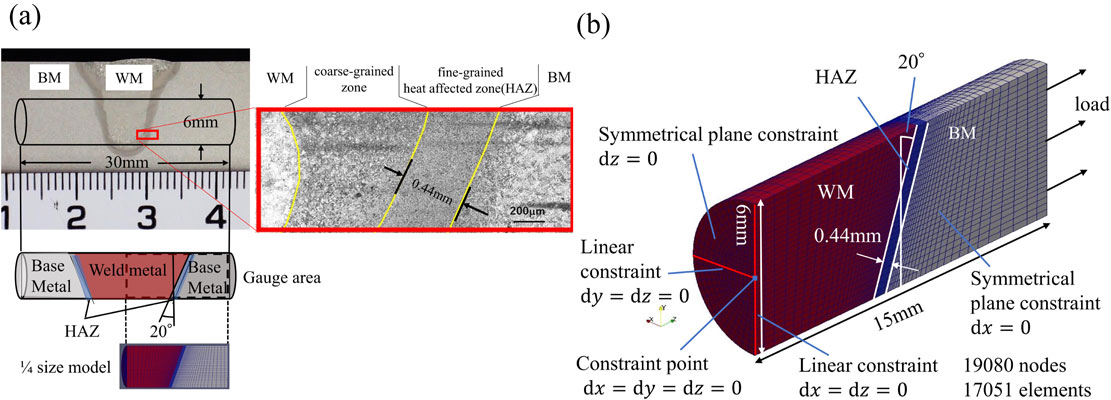
For a round rod specimen of the BM with a flange, we set the diameter of the gauge part to be 10 mm and the gauge length to be 50 mm, when we expect that the creep rupture time is relatively short. When we expect that the test time is long, we set the gauge length to 150 mm because the creep strain is expected to be extremely small. For the simulated HAZ and the WJ material, we set the gauge length and the diameter to be 30 and 6 mm, respectively, as a size compliant to JIS Z 2271, and for the simulated HAZ, we added a flange to measure its elongation. We prepared the WJ by means of Gas Tungsten Arc Weld and performed PWHT under the same conditions as for the simulated HAZ. We took a specimen from the WJ so that the WM part is located at the center of the gauge part. Figure 1(a) shows the shape of a prepared WJ and the location of a creep specimen taken from.

Fig. 1

(a) Photograph of the cross section of the weld, FEM model of uniaxial weld joint. (b) Boundary condition and element property for the FEM model.

We conducted the creep tests using a constant-load creep testing machine under the conditions shown in Table 1 for the BM, the simulated HAZ, and the WJ. We obtained the creep strain and the rupture time for the BM and the simulated HAZ, and the rupture time for the WJ besides the crept specimen. For the BM and the simulated HAZ, we divided the obtained elongation by the gauge length at the test start time, and we regarded that as the strain.

To numerically reproduce the creep test of the WJ by means of FEM, we produced a semi-cylindrical FEM model in which the symmetrical planes are set with the center plane perpendicular to the tensile direction and the plane cut along the center line parallel to the tensile direction, at the gauge part of the specimen. Figure 1(b) shows the constraint conditions, the load conditions, and the assignment of material properties to each element, for the FEM model that simulates the WJ specimen. Shape of the HAZ is obtained from the optical microscope observation of the etched welded cross section. There are two areas of the HAZ between the WM and the BM. Both zones are inclined at an angle of about 20° and the thickness of fine-grained zone within the HAZ was 0.44 mm. Considering this, we set the HAZ that penetrates the center of the FEM model obliquely. We generated grids composed of quadrilateral elements in the end of the tensile direction in the model, and projecting those shapes to the entire body, we assigned grids of hexahedral elements in the entire body. To make the grid spacing sufficiently fine in the HAZ and its vicinity, where we expect that the stress condition is inhomogeneous, we placed five elements in the longitudinal direction in the HAZ. In addition, in the regions in the BM and the WM that adjoin one of the two sides of the HAZ, we set the regions with their thicknesses the same as that of the HAZ, and we placed five elements in each region in the tensile direction. To suppress the total element number in the entire region, we make the grid spacing larger towards the end of the specimen. The number of nodes and elements in the produced FEM model is 19,080 and 17,051 respectively.

The creep parameters and the elastic constants given in each region are as follows: For the BM and HAZ, we used the material properties obtained from the tests of the BM and the simulated HAZ respectively. Although the material properties of the WM are unknown, we assumed that it has the same or similar degree of deformation as the BM, and decided to use the same material properties as those of the BM. In addition to the calculation for the WJ, for comparison, we performed calculations to simulate the creep tests of the BM and the simulated HAZ, assigning the properties of the BM or the HAZ to the entire FEM model.

2.2 Damage rule and creep constitutive equation

As a damage model, we use the time exhaustion rule (TER).⁸⁾ As an index that represents damage, we consider the amount of damage D_c for a certain element. This value is zero at the start of the test, and it gradually increases and becomes unity at the time of rupture. In the calculation of the FEM model, we determine that rupture occurs when the amount of damage becomes unity at a certain element. In addition, we call that element the rupture initiation element.

In the TER, we assume the increment of damage accumulated dD in an infinitesimal time interval dt as   

\begin{equation} \text{d}D = \frac{\text{d}t}{\mathit{Tr}(\sigma,T)}, \end{equation} (1)

where Tr(σ, T) is the rupture time at certain temperature T and stress σ. Generally speaking, the larger σ and the higher T, the shorter the rupture time becomes. The damage D_c(t₁) until a certain test time t₁ is given by integrating this with respect to time t as   

\begin{equation} D_{c}(t_{1}) = \int_{0}^{t_{1}}\frac{\text{d}t}{\mathit{Tr}(\sigma,T)}. \end{equation} (2)

In this study, we use a thermal activation power law for Tr(σ, T) as   

\begin{equation} \mathit{Tr}(\sigma,T) = A_{\text{TER}}\exp \left(\frac{Q_{\text{TER}}}{RT}\right)\sigma^{n_{\text{TER}}}, \end{equation} (3)

where Q_TER is the apparent activation energy of the rupture, n_TER is the stress index, A_TER is a constant, and R is the gas constant. We need to obtain these variables for each of the BM and the simulated HAZ. We linearize eq. (3) as:   

\begin{equation} \log (T_{r}(\sigma,T)) = \log (A_{\text{TER}}) + \frac{Q_{\text{TER}}}{RT} + n_{\text{TER}}\log(\sigma). \end{equation} (4)

Using the uniaxial creep test results of the BM and the simulated HAZ, we obtained Q_TER, n_TER, and A_TER for the BM and the simulated HAZ from the linear regression using logarithmic variables of temperature and stress.

An important issue is to set the scalar stress, on which the rupture time in the model depends. In a uniaxial creep test for a homogeneous material, the scalar stress is the test stress itself, but if we consider a material whose shape is as complex as a WJ and in which stress has multiaxiality, we need to appropriately set the scalar stress on which the rupture time depends. In this study, we examine three types of scalar stress: the maximum principal stress σ_maxp, the equivalent stress σ_eq, and the Huddleston stress⁹⁾ σ_Hud. If we denote the three orthogonal components of the diagonalized stress tensor, namely three components of the principle stresses, σ₁, σ₂, and σ₃ in descending order, these three types of scalar stresses are given as follows:   

\begin{equation} \sigma_{\text{maxp}} = \sigma_{1}, \end{equation} (5)

  

\begin{equation} \sigma_{\text{eq}} = \sqrt{((\sigma_{1} - \sigma_{2})^{2} + (\sigma_{2} - \sigma_{3})^{2} + (\sigma_{3} - \sigma_{1})^{2})/2}, \end{equation} (6)

  

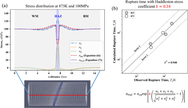
\begin{equation} \sigma_{\text{Hud}} = \sigma_{\text{eq}}\exp \left[b\left(\frac{\sigma_{1} + \sigma_{2} + \sigma_{3}}{\sqrt{\sigma_{1}^{2} + \sigma_{2}^{2} + \sigma_{3}^{2}}} - 1 \right) \right]. \end{equation} (7)

In a uniaxial creep test of a homogeneous material, in which stress does not have multiaxiality, all three stresses agree with each other.

For a coefficient b in the Huddleston stress, Huddleston proposed a recommended value as b = 0.24;⁹⁾ we also used the value in this study. However, we will examine a more appropriate value of the coefficient b in the discussion section.

As a creep constitutive equation, we used the Norton-Arrhenius type.¹³⁾ That is, we express the creep rate $\dot{\varepsilon }_{m}$ as a function of the equivalent stress σ_eq and the test temperature T as follows:   

\begin{equation} \dot{\varepsilon}_{m}(\sigma_{\text{eq}},T) = A_{\varepsilon}\exp \left(-\frac{Q_{\varepsilon}}{RT} \right)\sigma_{\text{eq}}^{n_{\varepsilon}}, \end{equation} (8)

where Q_ε is the apparent activation energy for the minimum creep rate, n_ε is the stress index, and the parameter A_ε is the material constant. In the same way as in eq. (3), we linearize eq. (8) as   

\begin{equation} \log(\dot{\varepsilon}_{m}(\sigma_{\text{eq}},T)) = \log (A_{\varepsilon}) - \frac{Q_{\varepsilon}}{RT} + n_{\varepsilon}\log (\sigma_{\text{eq}}), \end{equation} (9)

and we obtained Q_ε, n_ε, and A_ε using the linear regression for the uniaxial creep test results of the BM and the simulated HAZ.

3. Results

3.1 Creep test results, and determination of the material parameters of the BM and the simulated HAZ

Figure 2(a) and (c) are log-log plots of the minimum creep rate against the test stress for the BM and the simulated HAZ, respectively. We derived the minimum creep rate from the curve of the creep strain against time as the gradient of the region that can be approximated to be a linear line in the secondary creep stage. Figure 2(b) and (d) show log-log plots of the test stress against the rupture time for the BM and the simulated HAZ, respectively.

Fig. 2

Minimum creep rate versus testing stress ((a), (c)) and testing stress versus rupture times ((b), (d)) of uniaxial tests for base metal and HAZ, respectively. Gray lines for (a), (b) are regression lines using eq. (3) and eq. (9). The boundary of two regions is shown by a dashed gray line. Solid lines for (c), (d) are regression lines using eq. (3) and eq. (9). The gradient of inserted triangles corresponds to the stress exponent and the length of arrows between two regression lines of different temperatures corresponds to the apparent activation energy.

The dependence of the minimum creep rate on stress (each gradient of the test points for the same temperature in Fig. 2(a)) changes in the region between 100 and 120 MPa. Across this stress condition, within each region, the gradient of the minimum creep rate can be considered common regardless of temperature. Similarly, in the plot of the rupture time in Fig. 2(b), even though it is not so obvious, we can recognize the change of the gradient around 100 MPa. Since there is an inverse proportional relation between the minimum creep rate and the rupture time (Monkman-Grant law), it is reasonable to consider that both the minimum creep rate and the rupture time have the same stress level at which the stress dependence changes. Based on the multi-region analysis proposed by Maruyama et al.,¹⁴⁾ we divided the test region into the low-stress side and the high-stress side and applied a linear approximation to the rupture time and the minimum creep rate in each region. In Fig. 2(a) and (b), gray lines are regression lines of the low-stress side and the high-stress side. The thick light-gray dashed line normal to the stress axis is the region boundary, i.e., the line of 108 MPa, which is the crossing point of the two regression lines of the minimum creep rates at 823 K.

For the creep test results of the simulated HAZ (Fig. 2(c) and (d)), we have conducted creep tests of only five test conditions, it is difficult to discuss the multi region analysis. We assume there is only one region, and obtained parameters for each of the minimum creep rate and stress using linear regression. The gray solid lines are the regression lines. For both the BM and the simulated HAZ, the gradient of each regression line represents the stress index, and the interval in the regression line in the direction normal to the stress axis for each temperature corresponds to the temperature dependence.

To obtain Young’s modulus, for the BM, we used the elongation data obtained from the loading data at preparation of creep tests for the specimen heated to the test temperature. We used the values obtained by linear regression based on Hooke’s law, considering the data in the all stress condition at each temperature to be one sample. For determining the Young’s modulus of the HAZ, we used the elastic deformation part of each stress-strain curve obtained by tensile tests with the simulated HAZ specimens at 823 K and 873 K. For the Poisson ratio, we used the value at 293 K (20°C) of 2 1/4Cr–1Mo steel with stress relief treatment, described in a report.¹⁵⁾ Table 2 shows the creep and elastic parameters used in the FEM calculation.

Table 2 Creep and elastic parameters and test conditions under which they are applied in FEM calculation.

Figure 3(a) shows the log-log plot of the test stress against the observed rupture time for WJ specimens, with points marked by crosses. In the plot, for comparison, we plotted the rupture times of the simulated HAZ and those of the BM at 823 K in the range between 117 and 157 MPa, and at 873 K in the range between 78 and 98 MPa, by triangles and circles, respectively. As mentioned in the introduction, the rupture time of the WJ is located between the simulated HAZ and the BM.^6,7) In addition, in both temperature conditions, it seems that the stress index, gradient of the WJ rupture time against the stress, is closer to that for the simulated HAZ than that for the BM.

Fig. 3

Observed rupture time for weld joints, and those for base metal and HAZ around weld joint test conditions. (b) Photographs of ruptured specimen under the test conditions of 873 K and 100 MPa.

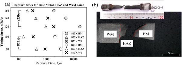
Figure 3(b) displays a photograph of a crept specimen at 873 K and 100 MPa. The rupture elongation and the reduction of area are large; therefore, it is difficult to analyze the fracture initiation position and crack propagation in detail, but we can recognize that the fracture initiated in the HAZ on the side of the BM, and the crack propagated along the BM-HAZ interface. Considering the fact that the stress index of the rupture time is close to that for the simulated HAZ, and also from the result of the rupture specimen observation, we can say that the type of the fracture of the WJ is of Type IV in every test condition. This tendency is consistent with existing reports.^4,6)

3.2 FEM calculation result

We performed FEM calculations for five test conditions that are the same as the WJ creep tests (see Table 1). When we use the parameters, the test stress at 823 K is on the high-stress side between 120 and 160 MPa, and the test stress at 873 K is on the low-stress side between 80 and 100 MPa; as shown in Table 2, we used parameters appropriate for each region. We performed FEM calculations by an in-house finite element analysis code,^10,16) developed by NIMS (National Institute for Materials Science) to perform damage analysis, using a supercomputer in NIMS and the Materials Integration System.^17,18)

Figure 4(a) shows the results of the rupture time of WJ tests by the FEM calculations. The thick dashed lines and the thin dotted lines represents the calculation results where we gave the properties of the BM and the simulated HAZ to all the elements. We confirmed that the simulations reproduced the creep test results to the same degree as the regression lines of the rupture time of BM and the simulated HAZ as shown in Fig. 2, respectively. Crosses show the creep test results, and diamonds, stars, and circles show the FEM calculation results, each of which uses the maximum principal stress, the equivalent stress, and the Huddleston stress as the scalar stress in the TER.

Fig. 4

(a) Observed and calculated rupture times of FEM damage analysis. Cross symbol is for the observed, and circle, star, and diamond symbols are for Huddleston, equivalent, and maximum principle stresses, respectively. Dashed and dotted lines are calculated rupture times of uniaxial tests for base metal and HAZ, respectively, simulated by FEM. (b) Observed and calculated rupture times for weld joint. Gray solid line represents 1:1 and gray dashed lines represent factor 2.

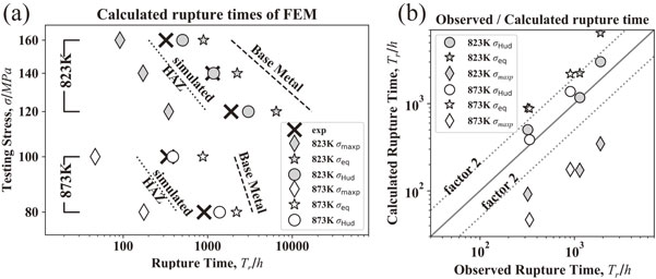
As mentioned in Sec. 3.1, the rupture time of the WJ tends to be longer than that of the simulated HAZ and shorter than that of the BM. In the FEM calculations, the equivalent stress and the Huddleston stress reproduced this qualitative tendency. The values of expected rupture time under the Huddleston stress are closest to the results of the creep tests. Figure 4(b) shows the comparison between these calculation results and the observed rupture time. The symbols are the same as in Fig. 4(a). The two dotted lines are where the ratio of the calculated rupture time to the observed rupture time becomes 2 and 0.5, respectively. All of the calculated rupture time under the Huddleston stress are within this range. Table 3 shows the rupture time in each test condition, the rupture time calculated in each scalar stress, and the ratio for each of them. The ratio is between 1.0 and 1.6 for the Huddleston stress, 1.9 and 3.4 for the equivalent stress, and between 0.1 and 0.3 for the maximum principal stress. As shown above, we found that the scalar stress that best reproduces the observed rupture times is the Huddleston stress. However, even using the Huddleston stress, the calculated rupture time is 1.6 times longer at the maximum, and we should be aware that the prediction is on the dangerous side.

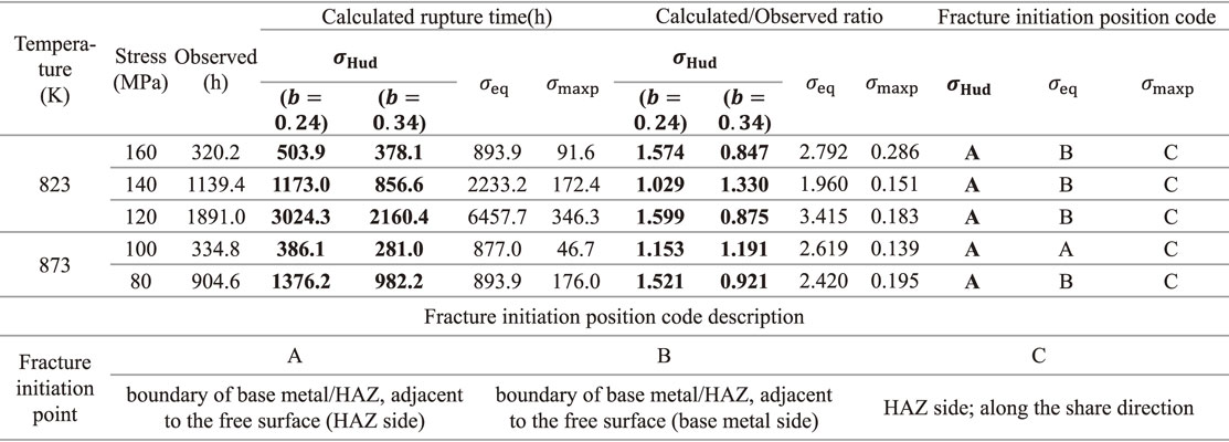
Table 3 Observed and calculated rupture times, with the original and optimized value of parameter b in the Huddleston stress, b = 0.24 and b = 0.34 respectively, and locations of fracture initiation position at the calculation for each test condition.

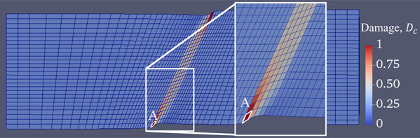
As a typical case, in Fig. 5, for the vicinity of the HAZ in the FEM model with conditions of 823 K and 120 MPa, we show a heat map for the damage D_c immediately after the rupture, evaluated with the three types of scalar stress and the rupture initiation elements in each scalar stress. To clarify the HAZ region, we show only nodes using points in the BM and the WM in the FEM model. We show the amount of damage from the minimum to the maximum using blue to red, respectively and the rupture initiation elements, that is, the elements where D_c = 1 are highlighted with pink borders. Since we gave the same material properties to the BM and the WM, and we placed the HAZ at the center of the model, the result of the heat map shows point symmetry around the HAZ. When we evaluate the damage with the maximum principal stress, the rupture time is short, there are several elements where D_c = 1 at the same time during a time step of the calculation.

Fig. 5

Comparison of rupture initiation element of FEM calculation. The HAZ region is shown as a solid surface with edges, while base metal and weld metal regions are shown in points. The rupture initiation element is shown with a pink edge. Heat map shows the accumulation of damage just after the rupture for each stress.

The rupture initiation elements under the Huddleston stress are located around the free surface adjoining the interface between the BM and the HAZ, on the side where the angle between the HAZ and the BM is an acute angle (the acute angle side). The damage accumulation is large around the rupture initiation elements, in the HAZ around the free surface, and the damage accumulation along the HAZ becomes smaller toward the inside of the model. In contrast, on the side where the HAZ adjoins the WM with an obtuse angle, the damage accumulation is extremely small. In addition, in the BM side next to the rupture initiation elements, there is not much damage accumulation. Similarly, in the case of the equivalent stress, the rupture initiation elements are located around the free surface in the BM-HAZ interface on the acute angle side of the HAZ, but most of the cases of rupture occurred on the BM side. The distribution of damage inside the HAZ is similar to that for the Huddleston stress, but the damage accumulation is large on the BM side around the rupture initiation elements. In contrast, in the case of the maximum principal stress, being clearly different from the cases of the Huddleston stress and the equivalent stress. Damage is accumulated along the line in the shearing direction that has an angle of 45° from the HAZ center, and the rupture initiation elements are located in the center of that region.

In Table 3, we summarize the rough locations of the fracture initiation position where is the location of rupture initiation elements in each of the stress and test conditions. The tendency of rupture locations as shown in Fig. 5 is almost the same in all of the test conditions, but in the case of the equivalent stress, we also observed a situation in which the rupture initiation elements are in the BM (and in the WM) rather than in the HAZ. However, even in this case, the rupture initiation elements adjoin the BM-HAZ interface (see Fig. 5 for the equivalent stress). In this way, in all of the test conditions in all of the three types of scalar stress, the following factors are common: the fracture initiation position is in the BM-HAZ interface, and the region where damage accumulation is high is along the HAZ. That is to say, in the FEM analysis of WJs in this study, we reproduced Type IV fracture regardless of the choice of stress.

4. Discussion

In the framework of the TER, we obtained a result that the rupture time evaluation using the Huddleston stress best reproduces the actual creep damage behavior.

The Huddleston stress is defined as the stress where the equivalent stress is multiplied by a coefficient derived from the three components of the principal stress, $H = \exp (b((\sigma _{1} + \sigma _{2} + \sigma _{3})/\sqrt{\sigma _{1}^{2} + \sigma _{2}^{2} + \sigma _{3}^{2}} - 1))$ (cf. eq. (7)). The parameter b in the exponent is a parameter to adjust the contribution of the hydrostatic pressure component (= (σ₁ + σ₂ + σ₃)/3).⁹⁾ When this hydrostatic pressure component represents tensile (a positive value, in this study), it is considered to promote the cavity formation, and when b is large, this means that we evaluate larger damage accumulation due to the cavity formation. In fact, when all of the three components of the principal stress are positive (tensile direction), the exponent is always larger than unity, and the Huddleston stress is inevitably larger than the equivalent stress. In this study, the equivalent stress controls the creep deformation (eq. (8)). We can understand that the damage evaluation using the Huddleston stress is designed so that the damage accumulation due to the creep deformation and the effect of the cavity formation^19,20) due to the hydrostatic pressure are superimposed together. In present section we will discuss how the shape of the HAZ and the stress distribution in the HAZ exert influences for the Huddleston stress. In the following discussion, to use the same elements where we evaluate stress, we use a test condition of 873 K and 100 MPa, where the rupture initiation elements are in the HAZ regardless of the type of stress. And for the stress analysis, we use the result at the rupture time under the Huddleston stress.

Figure 6 shows the three components of the principal stress tensor and the equivalent stress and the Huddleston stress calculated using those principle stresses along the center line of the FEM model (see the inset), immediately after the rupture time. To diagonalize a stress tensor, we used a function, numpy.linalg.eig of numpy 1.18.1 over Python 3.7.6. The stress distribution around the HAZ was significantly different between σ₁ and σ₂, σ₃. The maximum principal stress (σ_maxp = σ₁) is close to the testing stress 100 MPa in the end of the specimen near the uniaxial tensile condition, and it decreases once and then increases a little towards the HAZ; it apparently increases to a larger value of about 120 MPa in the HAZ. The stress in the HAZ becomes large because the cross section of the HAZ shrinks due to the elastic and creep deformations. In contrast, the values of σ₂ and σ₃ were almost zero in the end of the specimen, and they had negative values (compression direction) upon approaching the HAZ. Then, in the HAZ, they changed to very large positive values and σ₂ and σ₃ were about 73 and 51 MPa, respectively. We can understand that these peculiar distributions of σ₂ and σ₃ across the HAZ are due to the difference of the deformation behavior between the HAZ and the BM. HAZ has a smaller Young’s modulus compared to the BM, which makes the elastic deformation larger, and in addition, the rate of the creep deformation becomes larger. Therefore, the HAZ is significantly deformed and the cross section becomes smaller. Because of this, to keep strain compatibility at the BM-HAZ interface, the internal stress is generated in the direction to suppress the cross-sectional contraction on the HAZ side, and in the direction to facilitate the cross-sectional contraction on the BM side. We can interpret that the large intermediate and minimum principal stresses are generated in the HAZ due to the constraint from the BM.

Fig. 6

Distributions of three principle stresses σ₁, σ₂, and σ₃, equivalent stress σ_eq, and Huddleston stress σ_Hud along the central axis (Z order) of the FEM model shown in the inset, just after the rupture, under the testing conditions of 873 K and 100 MPa.

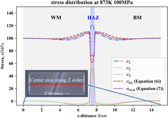
In this way, because of the multiaxiality of the stress generated due to the difference in the deformation behavior between the HAZ and the BM, the equivalent stress in the HAZ eventually becomes small, at about 62 MPa, which is much smaller than the testing stress, 100 MPa. On the other hand, the coefficient H for the Huddleston stress becomes 1.16 due to a positive hydrostatic pressure component so the Huddleston stress becomes around 72 MPa, which is larger than the equivalent stress; however, it is still lower than the testing stress. As seen in the above analysis, we can qualitatively explain the result that the rupture time of the WJ becomes longer than that of the simulated HAZ, if we consider that the accumulation of damage of the WJ is delayed due to that the deformation of HAZ in the WJ is subjected to the constraint from the BM, which makes the rate of the creep deformation smaller than that in the case of the simulated HAZ.

Let us further examine in detail the inhomogeneous deformation behavior in the HAZ. Figure 7 shows the displacement in the model, by magnifying the displacement 10 times larger. First, we find that, with respect to the tensile direction of the specimen, the HAZ shows shear deformation in the same direction as the inclination of the HAZ. When the HAZ is inclined, shear deformation can generate displacement in the direction of the load, without being affected by the deformation constraint from the BM. In an actual creep test, the HAZ exhibited a large shear deformation (Fig. 3(b)). The inset shows a magnified view in the vicinity of the free surface in the HAZ end including a rupture initiation element (element A). The shear deformation is largest at element A, which is on the acute angle side of the free surface, which can be connected to the fact that the damage accumulates at the highest rate.

Fig. 7

Displacement of the model at the rupture time with Huddleston stress under the test conditions of 873 K and 100 MPa. Projected heat map shows the distribution of damage by Huddleston stress. Outlined cells are the rupture initiation element (A) within the HAZ. The inset is the enlarged view of the white rectangle region around HAZ.

That is, basically, the damage accumulates rapidly where the creep deformation occurs easily. However, quantitatively compared with the observed rupture time, when we evaluated damage using the equivalent stress that regulates the creep deformation, the rupture time calculated became quite long, and the prediction was on the dangerous side. As already mentioned, with regard to the rupture time, the Huddleston stress gives better reproducibility of the tests. Considering the fact that the Huddleston stress is obtained by multiplying the equivalent stress by the coefficient H including the hydrostatic pressure, we need to consider not only the damage accumulation due to the creep deformation, but also the effect that the cavity formation due to a positive hydrostatic pressure accelerates the damage accumulation.

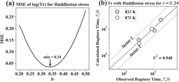
Based on what has been mentioned above, we examine how much we need to take the hydrostatic pressure component into account for 2 1/4Cr–1Mo steel, which we have been studying in this research. Parameter b in the coefficient H is important, and this value is an index that represents how much we take the hydrostatic pressure component into account. Here, we will obtain the optimum value of the parameter b that reproduces the rupture times obtained in the tests in all of the test conditions as much as possible. For the log(Tr_Hud(b)), which is the logarithm of the rupture time Tr_Hud(b) evaluated using the Huddleston stress, and the logarithm of observed rupture time, log(Tr_obs), we evaluated the mean squared error (MSE), which is the sum of the square of the error throughout all five testing conditions, that is,   

\begin{equation} \mathit{MSE}(b) = \frac{\displaystyle\sum (\log (\mathit{Tr}_{\text{obs}}) - \log (\mathit{Tr}_{\text{Hud}}(b)))^{2}}{5}, \end{equation} (10)

to be an error function, and we aimed to minimize this. To derive this precisely, we need to perform the FEM analysis by varying b at small intervals, but since the FEM calculation takes a long time, we obtained MSE(b) by reusing the calculated results (for details, see Appendix). In Fig. 8(a), we plot MSE(b) against the value of b from 0.20 to 0.50. In this range, MSE(b) has a unimodal downward-convex curve, and the value of b that gives the minimum value is b = 0.34, considering the significant figures to be two decimal places. Using this new value of b, we performed the FEM analysis again, and, we show the results of the damage evaluated using Huddleston stress to compare the tests in Table 3 and Fig. 8(b). We see that the calculation results reproduced the creep test results extremely well. The determination coefficient that represents the degree of replication between the observed and the calculated rupture time is R² = 0.804 for b = 0.24, while it is R² = 0.948 for b = 0.34, from which we find that improving b makes the reproducibility better. The ratio of the calculated rupture time to the test one is 1.33 at maximum, which is sufficiently smaller than the previous calculating result.

Fig. 8

(a) MSE between observed rupture time and calculated rupture time with Huddleston stress versus b from 0.20 to 0.50. The value of b that gives the minimum of MSE is 0.34. (b) Calculated rupture times by FEM with Huddleston stress, with b = 0.34.

We found that for 2 1/4Cr–1Mo steel, b = 0.34, which is larger than the value in an existing study,⁹⁾ is appropriate. Note that, in this study, we regarded b as a value that does not depend on the test temperature and stress, but we should be aware that this is just an approximation. The cavity formation due to the hydrostatic pressure is controlled by a diffusion phenomenon;²¹⁾ therefore, we can consider that b depends on the test temperature and the test stress. We expect that considering this enables us to make a more accurate prediction.

5. Conclusions

To establish a technology to predict the rupture time of a WJ made from heat-resistant 2 1/4Cr–1Mo steel that has a complex stress distribution near the HAZ, we have examined a damage model that has high test reproducibility. We have obtained material properties from creep tests of the BM and the simulated HAZ, and obtained the rupture time and the fracture type from creep tests of round rod WJs. From these results, deriving the material properties of the BM and the simulated HAZ, we have performed high-accuracy creep test simulations using an FEM model that simulates a WJ creep specimen. Comparing the tests and the calculation results, we have examined the scalar stress that is appropriate under the framework of the TER. As a result, we obtained the following conclusions.

• (1)    The fracture type of the creep tests has been determined to be Type IV that begins on the BM side of the HAZ and proceeds along the BM-HAZ interface. In contrast, the location at which rupture is initiated in the calculations is as follows: For the Huddleston stress and the equivalent stress, this location is around the free surface in the BM-HAZ interface on the side where the HAZ is inclined at an acute angle. For the maximum principal stress, it is the region in the shear direction with an angle of 45° from the HAZ center. In both cases, the locations where rupture is initiated are in the BM-HAZ interface, and the regions where damage accumulates are along the HAZ. Therefore, in all types of scalar stress, Type IV fracture has been reproduced.
• (2)    The rupture time ratio obtained in the creep tests is in the following order: simulated HAZ < the WJ < the BM, and the scalar stresses in the calculations that satisfy this relation are the equivalent stress and the Huddleston stress. Among them, the scalar stress that gives the rupture time closest to the result of the WJ creep test is the Huddleston stress.
• (3)    From the analysis of the stress tensor, we can understand that the rupture time of the WJ is longer than that of the simulated HAZ because a positive hydrostatic pressure component is generated in the HAZ due to the deformation constraint by the BM and the WM. The damage accumulates where the large shear deformation occurs within the HAZ, i.e. at the free surface.
• (4)    The equivalent stress that regulates the creep deformation gives a prediction on the dangerous side. Since the Huddleston stress in which the damage acceleration due to the hydrostatic pressure in the tensile direction is taken into consideration gives results closer to the observed rupture time, we can conclude that we need to consider the cavity formation due to the hydrostatic pressure in the tensile direction as a factor that accelerates damage.
• (5)    For the steel and the test conditions in this study, the rupture time is determined by the balance between two factors: the creep deformation and the cavity formation due to the tensile hydrostatic pressure. Based on this conclusion, we have optimized the parameter b that adjusts the contribution of the hydrostatic pressure component for the Huddleston stress to best reproduce the test values. By setting b = 0.34, which is larger than the value in an existing report, the coefficient of determination for the creep test results has been greatly improved to R² = 0.948, and the reproducibility of tests has been enhanced.

Acknowledgment

This work was supported by the Council for Science, Technology and Innovation (CSTI), Cross-ministerial Strategic Innovation Promotion Program (SIP), “Materials Integration for Revolutionary Design System of Structural Materials” (funding agency: JST).

REFERENCES

• 1)   J.A.  Francis,  W.  Mazur and  H.K.D.H.  Bhadeshia: Mater. Sci. Technol. 22 (2006) 1387–1395.
• 2)   P.K.  Liaw,  M.G.  Burke,  A.  Saxena and  J.D.  Landes: Metall. Trans. A 22 (1991) 455–468.
• 3)   F.  Kawashima,  T.  Tokuyoshi,  T  Igari,  A.  Shibashi and  N.  Tada: J. Soc. Mater. Sci. Japan 52 (2003) 631–638.
• 4)   Y.  Li,  H.  Hongo,  M.  Tabuchi,  Y.  Takahashi and  Y.  Monma: Int. J. Press. Vessels Piping 86 (2009) 585–592.
• 5)   K.  Laha,  K.S.  Chandravathi,  K.B.S.  Rao,  S.L.  Mannan and  D.H.  Sastry: Int. J. Press. Vessels Piping 77 (2000) 761–769.
• 6)   T.  Ogata and  M.  Yaguchi: J. Soc. Mater. Sci. Japan 47 (1998) 253–259.
• 7)   F.  Abe and  M.  Tabuchi: Sci. Technol. Weld. Joining 9 (2004) 22–30.
• 8)   M.W.  Spindler: Mater. Sci. Technol. 23 (2007) 1461–1470.
• 9)   R.L.  Huddleston: J. Press. Vessel Technol. 107 (1985) 421–429.
• 10)   T.  Watanabe,  M.  Tabuchi,  M.  Yamazaki,  H.  Hongo and  T.  Tanabe: Int. J. Press. Vessels Piping 83 (2006) 63–71.
• 11)   K.  Koiwa,  M.  Tabuchi,  M.  Demura,  M.  Yamazaki and  M.  Watanabe: Mater. Trans. 60 (2019) 213–221.
• 12)   M.  Demura and  T.  Koseki: Mater. Trans. 61 (2020) 2041–2046.
• 13)  M.E. Kassner: Fundamentals of Creep in Metals and Alloys, 3.ed., (Butterworth-Heinemann, Oxford, 2015).
• 14)   K.  Maruyama,  J.  Nakamura,  N.  Sekido and  K.  Yoshimi: Mater. Sci. Eng. A 696 (2017) 104–112.
• 15)  H. Kimura, H. Sugaya, E. Yoshida and Y. Wada: PNC TN9410 90-094, (JNCDI Technical Cooperation Section, 1990) p. 65 (online).
• 16)   H.  Hongo,  M.  Tabuchi and  T.  Watanabe: Metall. Mater. Trans. A 43 (2012) 1163–1173.
• 17)   M.  Demura and  T.  Koseki: Materia Japan 58 (2019) 489–493.
• 18)   S.  Minamoto,  T.  Kadohira,  K.  Ito and  M.  Watanabe: Materia Japan 58 (2019) 511–514.
• 19)   A.J.  Perry: J. Mater. Sci. 9 (1974) 1016–1039.
• 20)   W.D.  Nix,  J.C.  Earthman,  G.  Eggler and  B.  Ilschner: Acta Metall. 37 (1989) 1067–1077.
• 21)   A.T.  Yokobori, Jr.,  K.  Abe,  H.  Tsukidate,  T.  Ohmi,  R.  Sugiura and  H.  Ishikawa: Mater. High Temp. 28 (2011) 126–136.

Appendix

We explain how to recalculate the rupture time under the framework of the TER, using the FEM calculation results that have already been obtained.

In the framework of the TER we considered in this study, there is no need to feedback the damage calculation result to the FEM calculation; therefore, using the time series of the stress tensor that has already been calculated for a certain element, we can recalculate the Huddleston stress with an arbitrary b for that element. It is inefficient to recalculate the Huddleston stress for all of the elements. If the elements where the rupture occurs are determined, using the time series data of the Huddleston stress for those elements, we can calculate the rupture time for an arbitrary b. What we need to focus on is at which element the rupture occurs, but as mentioned above, the rupture initiation element is around the free surface in the BM-HAZ interface, on the side where the HAZ adjoins the BM with an acute angle (the acute angle side). If we assume that the rupture initiation element does not change when the value of b is varied, we can perform the calculation using the history of the stress tensor for the rupture initiation element that we consider.

In Table A1, we show the comparison between the rupture time obtained in the above calculation using b = 0.24 and the rupture time obtained by the FEM using b = 0.24. The rupture time calculated from the stress tensor for the rupture initiation element is slightly longer, but this difference can be considered to depend on the error treatment in the calculation between the FEM calculation and the Python library that we used this time. The determination coefficient for the logarithm of both rupture time is R² = 0.99 and over, and we consider that this difference is sufficiently small.

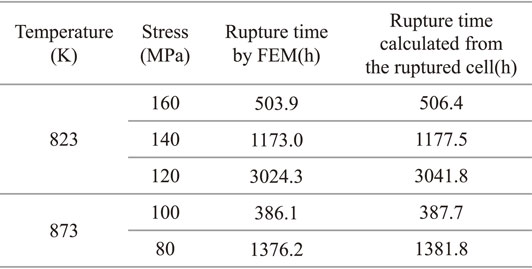
Table A1 Comparison of the rupture time by FEM with the rupture time calculated from the time series of stress tensor of ruptured cell with b = 0.24.