Abstract
The temper rolling process of hot-rolled strips is the final rolling step to improve the flatness of the strips and shape slippage of the coiled strips. Poor flatness of a hot-rolled strip causes lateral movement of the strip during the temper rolling process. Manual leveling operations to control this movement result in a much lower line speed and productivity. Moreover, the quality of manual leveling is not consistent, as it depends on the operator’s experience. Lack of understanding of the lateral movement phenomenon has sustained manual operation and discouraged the development of an automatic control system. To solve this problem, the authors propose both a new lateral movement model and a theoretical method. A lateral movement model for temper rolling and a large-deflection strip model are important components in the new model. In the method, lateral movement stability is equivalent to an eigenvalue problem with lateral movement static equations. Their usefulness is confirmed by comparing the results of experimental rolling in the laboratory with those of numerical calculations. The simulation results obtained using the proposed models confirm that actual problems can be solved more exactly than with the conventional linear model. Thus, simulation using the proposed models can support the investigation of lateral movement problems and the development of an automatic control system.
This Paper was Originally Published in Japanese in J. Jpn. Soc. Technol. Plast. 61 (2020) 107–114. The captions of figures were slightly modified.
1. Introduction
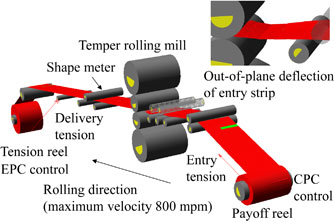
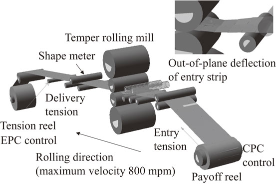
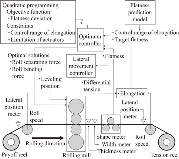
The temper rolling process of hot-rolled steel strips, which improves the flatness of the strips and shape slippage of the coiled strips, prevents lateral movement of hot-rolled strips in downstream process lines. Figure 1 shows a developed control system of a temper rolling line. The automatic control system provides elongation setup based on a shape prediction model,1) dynamic control of flatness and elongation2) and control of lateral movement. The shape prediction model predicts the strip shape at the mill entry side by using physical models and sensing data in the hot rolling process. Elongation setup outputs the tolerance range of elongation based on the predicted strip shape at the entry side. Dynamic control of flatness and elongation controls the strip flatness to zero within the tolerance range of elongation. In this development, a strip lateral movement simulator for the temper rolling line, as shown in Fig. 2, was also developed. This numerical simulator makes it possible to assess the performance of the logic and the robustness of lateral movement control, and also enables assessment of operational conditions such as a strip tension. Its background theories are described in detail in the following.
A strip sometimes appears to move in the lateral direction during rolling with a rolling mill.3) Because this lateral movement causes lower productivity and the work-roll damage, many researchers and engineers have studied and analyzed lateral movement in hot-strip4,5) and cold-strip3,6) rolling. A lateral movement analysis for strip rolling requires a coupled analysis of the strip lateral movement at the rolling mill and a model of strip deflection at the mill entry and delivery sides. In general, a beam model is used in the strip deflection model.3,6) The beam model is tuned to represent the actual results considering strip buckling. For example, bending stiffness is tuned to be smaller. On the other hand, from the viewpoints of calculation time and convergence, the coupled analysis7) of microscopic rolling phenomena and the standard elastic shell model is practically difficult.
A large-deflection strip model8) and a large-deflection discrete strip model9) have been developed to solve the above problems. The first model can be applied to a straight path and elastic bending and is formulated by approximating an elastic plate model. The second model can be applied to a curved path and elasto-plastic bending. The simulator shown in Fig. 2 represents the simulator based on the large-deflection discrete strip model. In the present study, a new lateral movement model (LMM) for temper rolling is derived from the approximation model for cold-strip rolling, considering the temper rolling reduction is very small. A LMM for a temper rolling line with payoff, rolling and coiling processes, is proposed, and its usefulness is confirmed by comparing the theoretical results, the results of experimental rolling in the laboratory and the results of numerical calculations. A lateral movement simulation of the simplex coiling process calculated by a general FEM has already been presented,10) but lateral movement simulation of a complex process such as a temper rolling line, including the payoff, rolling and coiling processes, is the first trial.
2. Lateral Movement Model of Temper Rolling Line
2.1 Outline of model
Figure 3 shows the experimental rolling line to clarify the proposed LMM. The line comprises a 2-high rolling mill, a payoff reel, a tension reel and deflector rolls at the entry and delivery sides. The LMM is solved by using either MATLAB/Simulink or MSC.ADAMS. The former has better compatibility with the large-deflection strip model,8) whereas the latter is a general analysis application for multi-body dynamics and has better compatibility with the large-deflection discrete strip model.9) The simulator in Fig. 2 was built on MSC.ADAMS. The modeling and calculation time of a simulator on MATLAB/Simulink is shorter. Each model on Simulink is represented as a block diagram. The block provides the model calculation and interface ports which input and output information such as forces and velocities. The block is represented by a state-space model and is described as a S-Function. The blocks represent the LMM at a payoff reel, referring to Appendix A2, the strip model at the entry side, the LMM of the temper mill, the strip model at the delivery side and the LMM at a tension reel with a boundary condition of simple support considering the deflector roll. These blocks are arranged in the order of strip movement. The unit system in this paper is the SI unit system.
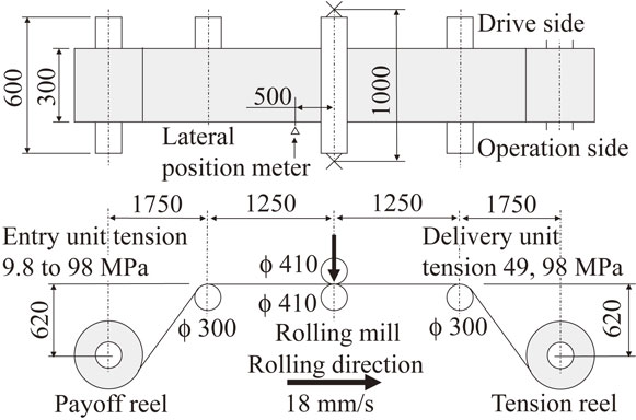
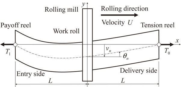
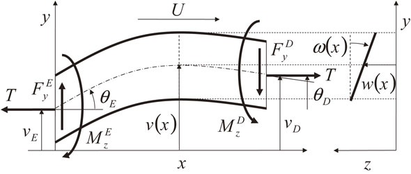
Figure 4 shows the schematic of strip lateral movement in temper rolling. The x-axis shows the strip rolling direction, and the y-axis shows the lateral direction. The LMM for cold rolling is formulated by using the Bland & Ford formula, which is an approximation of cold rolling. The LMM for temper rolling is formulated by simplifying the LMM for cold rolling, considering the very small reduction of the strip in temper rolling.
The work rolls of a rolling mill grip a strip. Assuming the strip velocity in the lateral direction is zero (non-slip), the constraint3,6) is given by
| \begin{equation}
Dv_{n}/Dt = dv_{n}/dt + U\theta_{n} = 0
\end{equation}
| (1) |
where
t is time,
vn is the strip lateral displacement at the mill, θ
n is the strip orientation angle and
U is the rolling velocity. When rolling an oriented strip, the strip appears to be moving in the lateral direction.
Considering the very small reduction in temper rolling and approximating the forward slip equation of Bland & Ford11) according to the formulation described in Appendix A1, the strip orientation angle velocity is given by
| \begin{equation}
\frac{d\theta_{n}}{dt} = U\left\{- \frac{3}{4A}(h_{0df} - h_{1df}) + \frac{\beta_{M0}}{kI}M_{0} - \frac{\beta_{M1}}{kI}M_{1} - \kappa_{1} \right\}
\end{equation}
| (2) |
where
h0df and
h1df are the wedges of the delivery and entry strip,
M0 and
M1 are the in-plane moment acting on the delivery and entry strip, κ
1 is the camber curvature of the entry strip,
A is the strip cross-sectional area and
I is the second moment of strip area.
A and
I are approximated as
hb and
hb3/12 when the wedge is very much smaller than the strip thickness
h, where
b is the strip width.
k is the strip deformation resistance. β
M0 and β
M1 show the influence coefficients of the delivery moment
M0 and the entry moment
M1. They are represented respectively by
| \begin{equation*}
\beta_{M0} = \frac{\sqrt{h/R'}}{4\mu \{1 - (T_{0} - 2\mu P_{0}^{e})/(kA)\}}\sqrt{r},
\end{equation*}
|
| \begin{equation*}
\beta_{M1} = \frac{\sqrt{h/R'}}{4\mu \{1 - (T_{1} - 2\mu P_{1}^{e})/(kA)\}}\sqrt{r}
\end{equation*}
|
where μ is the friction coefficient,
R′ is the radius of the flattening work roll,
r is the reduction in thickness,
T0 and
T1 are the tensions acting on the delivery and entry strip and
$P_{0}^{e}$ and
$P_{1}^{e}$ are the roll separating force
11) at the elastic recovery and compression zones.
Considering the plastic action on the rolled strip and the mill stiffness, the equation for the delivery wedge4) is given by
| \begin{align}
h_{0df} & = \frac{1}{K_{l} + M_{l}}\biggl\{\frac{2bP}{b_{l}{}^{2}}v_{n} + \frac{bK_{l}}{b_{l}}S_{df} + M_{l}h_{1df}\\
&\quad - \frac{16bh_{r}K_{l}}{b_{r}{}^{2}}v_{n} + \frac{P}{khb_{l}{}^{2}(1 - \alpha_{c})}(M_{0} + M_{1})\biggr\}
\end{align}
| (3) |
where
Sdf is the difference in mill leveling, and
P is the roll separating force which contributes to strip rolling based on Hill’s formula
11) and is represented by
| \begin{equation*}
P = \left\{1.08 + r\left(1.79\mu \sqrt{\frac{R'}{h}} - 1.02 \right) \right\}k(1 - \alpha_{c})b\sqrt{R'hr}.
\end{equation*}
|
is the distance between the work-roll chocks,
br is the width of the work-roll barrel,
hr is the center deflection of the work-roll barrel,
Kl is the mill leveling stiffness and
Ml is the strip leveling stiffness represented by
| \begin{equation*}
M_{l} = \left\{0.54 + \frac{3r}{2}\left(1.79\mu \sqrt{\frac{R'}{h}} - 1.02 \right) \right\}\frac{k(1 - \alpha_{c})b^{3}}{6b_{l}{}^{2}}\sqrt{\frac{R'}{rh}}.
\end{equation*}
|
α
c is the coefficient of the tension effect and is represented by
| \begin{equation*}
\alpha_{c} = (T_{0} + T_{1} - 2\mu P_{0}^{e} - 2\mu P_{1}^{e})/(2kA).
\end{equation*}
|
Adding the camber curvature by rolling to the entry camber curvature κ1, the delivery camber curvature4) κ0 is given by
| \begin{equation}
\kappa_{0} = (h_{0df} - h_{1df})/A + \kappa_{1}.
\end{equation}
| (4) |
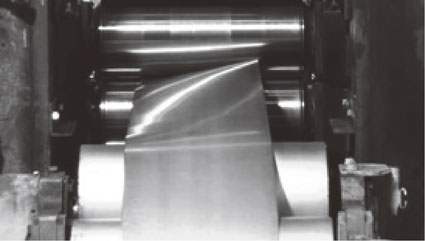
The large-deflection strip model,8) which is an approximated model of the large-deflection plate model, is applied to simulations on MATLAB/Simulink as the strip deflection model. To shorten the calculation time, it is assumed that the strip model does not flow in the strip rolling direction within the analysis space (pseudo-Euler form). A FEM analysis of the plate model makes the process of camber flow difficult, and the many elements necessary in order to secure the convergence of a large-deflection FEM analysis result in a longer calculation time. On the other hand, using a basic beam model shortens the calculation time and improves the convergence of calculation, but the beam model prevents precise simulations. Therefore, we applied the large-deflection strip model, which is a specialized model for lateral movement problems and calculates out-of-plane elastic deflection with bending and twist, as shown in Fig. 5. The functional of the large-deflection strip model shown in Fig. 6 and the boundary conditions are given by
| \begin{align}
\Pi & = \int_{0}^{L}\bigg\{\frac{EI}{2}(\cos \omega (\partial_{xx}v) + \sin \omega (\partial_{xx}w) - \kappa)^{2} \\
&\quad+ \frac{T}{2}(\partial_{x}v)^{2} \bigg\}dx\\
&\quad + \int_{0}^{L}\bigg\{\frac{Db}{2}(\sin \omega (\partial_{xx}v) - \cos \omega (\partial_{xx}w))^{2}\\
&\quad + \frac{T}{2}(\partial_{x}w)^{2} \bigg\}dx\\
&\quad + \int_{0}^{L}\bigg\{\frac{Db^{3}}{24}(\partial_{xx}\omega)^{2} + \left((1 - \nu)Db + \frac{Tb^{2}}{24} \right)(\partial_{x}\omega)^{2} \\
&\quad + \frac{Ehb^{5}}{1440}(\partial_{x}\omega)^{4} \bigg\}dx\\
&\quad + M_{z}^{E}(\partial_{x}v(t,0) - \theta_{E}) - M_{z}^{D}(\partial_{x}v(t,L) - \theta_{D})\\
&\quad - F_{y}^{E}(v(t,0) - v_{E}) + F_{y}^{D}(v(t,L) - v_{D}),\\
&\quad w(t,0) = w(t,L) = \partial_{x}w(t,0) = \partial_{x}w(t,L) = 0,\\
&\quad \omega (t,0) = \omega (t,L) = \partial_{x}\omega (t,0) = \partial_{x}\omega (t,L) = 0
\end{align}
| (5) |
where
L is the strip length,
v is lateral deflection,
w is vertical deflection, ω is the torsion angle, ν is the Poisson ratio,
E is Young’s modulus.
D is the bending rigidity and is defined as
| \begin{equation*}
D = Eh^{3}/12 \times (1 - \nu^{2})^{-1}.
\end{equation*}
|
is tension, κ is the camber curvature that flows within the strip,
$M_{z}^{E}$ and
$M_{z}^{D}$ are the in-plane moments at the entry and delivery sides,
$F_{y}^{E}$ and
$F_{y}^{D}$ are the lateral shearing forces at the entry and delivery sides, θ
E and θ
D are the orientation angles at the entry and delivery sides and
vE and
vD are the lateral displacements at the entry and delivery sides. In this paper, the first-order partial derivative of a function
v with respect to the variable
x is denoted by ∂
xv.
Equation (5) shows that deflections
v and
w are independent (in-plane deflections) if the torsion angle ω is constrained to be zero, whereas the deflection
v interacts nonlinearly with deflection
w by the medium of the torsion angle ω (out-of-plane deflection).
The large-deflection strip model shown in Fig. 6 is calculated nonlinearly by using the Rayleigh-Ritz method.12) This calculation process is implemented by using a function of the MEX S-Function, where the calculation of the tangent stiffness matrix and a solver of the system of linear equations are programmed by using C/C++ language to shorten the calculation time.
The block diagram of the strip deflection model interacts with the block diagrams of the LMM at the mill or on the rolls through their information of forces and velocities. The advection equation of the camber curvature within a strip
| \begin{equation*}
D\kappa/Dt = \partial_{t}\kappa + U\partial_{x}\kappa = 0
\end{equation*}
|
is calculated by using the CIP method, which enables fast convergence of calculation.
3. Experimental Rolling in Laboratory and Clarification of Models
3.1 Experimental rolling in laboratory
The bifurcation point, where the path of lateral movement changes from convergence to divergence with a decrease of entry tension, is known.13) Here, the validity of the LMM of the temper rolling line is clarified by performing experimental rolling in the laboratory and comparing the experimental results of the bifurcation point with the theoretical results.
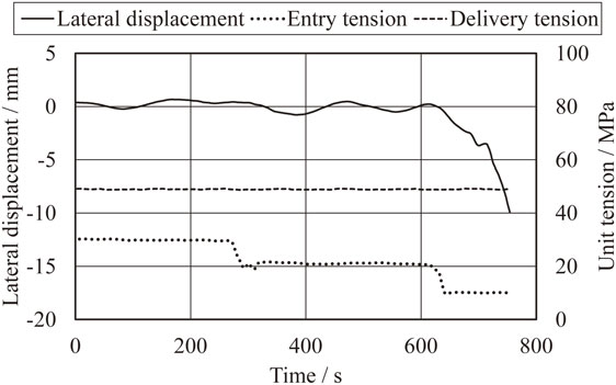
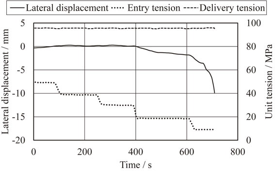
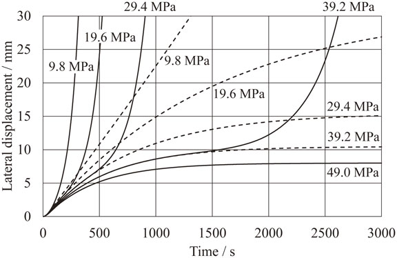
Table 1 shows the experimental rolling conditions. The underlined values are the values of the experimental conditions. First, steel strip rolling was stabilized without lateral movement in the initial state of the experiments. The entry and delivery unit tensions were set to be 49 MPa, and the lateral displacement at the mill in manual leveling was set so as to achieve a convergence of within 3 mm. Experimental rolling was started after the entry unit tension was set to 29 MPa, and the entry tension was then decreased stepwise during rolling while monitoring the strip lateral movement. Rolling was stopped when the lateral displacement at the mill exceeded a specified value. Figure 7 shows the results of this experiment, where the vertical axis shows the lateral displacement at the mill and the horizontal axis shows time. The path of the lateral displacement converged when the entry unit tension was above 20 MPa, and diverged when the entry unit tension was below 10 MPa. The elongation in this experiment was about 1.5%. Figure 8 shows the experimental results when the delivery unit tension was set to 98 MPa and the other experimental conditions were the same as those shown in Fig. 7. The path of the lateral displacement converged when the entry unit tension was above 20 MPa, and diverged when the entry unit tension was below 10 MPa. Lateral displacement seemed to increase gradually when the entry unit tension was 20 MPa. The elongation in this experiment was about 2.0%.
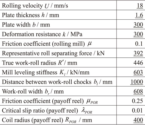
Table 1 Experimental rolling conditions.
These experiments confirmed that the critical entry tension, which is the smallest tension for maintaining stable lateral movement, existed at the bifurcation point. The critical entry tension slightly increased and lateral movement seemed to become slightly unstable when the delivery tension was larger. Hence, it is considered that the delivery tension did not seriously affect the phenomena of lateral movement in these experiments.
3.2 Clarification of LMM by eigenvalue analysis for steady state of lateral movement
In this section, the mechanism of the experimental phenomena is theoretically analyzed by using lateral movement equations. It is considered that lateral deflection converges if the steady state of lateral movement3) exists and diverges if it does not exist. Figure 4 shows the schematic of the analyzed lateral movement. The strips at the entry and delivery sides are assumed to be an elastic beam (restricted to in-plane bending) with the length of L. Considering the bias errors are zero, i.e.,
| \begin{equation*}
h_{1df} = 0,\quad \kappa_{1} = 0,\quad S_{df} = 0
\end{equation*}
|
and the equations are steady (i.e., the time derivative is zero), the lateral velocity constraint of
eq. (1) and the orientation angle velocity of
eq. (2) become
| \begin{equation}
\theta_{n} = \partial_{x}v_{0}(0) = 0,
\end{equation}
| (6) |
| \begin{equation}
- \frac{3}{4}h_{0df} + \frac{12\beta_{M0}}{kb^{2}}M_{0} - \frac{12\beta_{M1}}{kb^{2}}M_{1} = 0
\end{equation}
| (7) |
where
v0 is the lateral deflection of the delivery beam. Considering the bias errors to be zero,
eq. (3) of the delivery wedge becomes
| \begin{equation}
h_{0df} = \gamma v_{n} + \tau (M_{0} + M_{1})
\end{equation}
| (8) |
where γ and τ are the influence coefficient of the lateral displacement
vn and the sum of the entry and delivery moments, respectively. As
eq. (8) agrees with
eq. (3), γ and τ become
| \begin{align*}
\gamma &= \frac{2b}{K_{l} + M_{l}}\left(\frac{P}{b_{l}{}^{2}} - \frac{8h_{r}K_{l}}{b_{r}{}^{2}} \right), \\
\tau &= \frac{P}{khb_{l}{}^{2}(1 - \alpha_{c})(K_{l} + M_{l})}.
\end{align*}
|
Substituting
eq. (8) in
eq. (7),
eq. (7) becomes
| \begin{equation}
- \gamma v_{n} - S_{0}M_{0} - S_{1}M_{1} = 0
\end{equation}
| (9) |
where
| \begin{equation*}
S_{0} = \tau - 16\beta_{M0}/(kb^{2}),\quad S_{1} = \tau + 16\beta_{M1}/(kb^{2}).
\end{equation*}
|
The lateral deflection equation of the entry beam is given by
| \begin{equation}
EI\partial_{xxxx}v_{1} - T_{1}\partial_{xx}v_{1} = 0\quad (- L \leq x \leq 0)
\end{equation}
| (10) |
where
v1 is the lateral deflection of the entry beam. The lateral deflection equation of the delivery beam is given by
| \begin{equation}
EI\partial_{xxxx}v_{0} - T_{0}\partial_{xx}v_{0} = 0\quad (0 \leq x \leq L).
\end{equation}
| (11) |
Considering the fact that the coiled strips on the payoff reel are rubbed together with a very small slip rate, the boundary conditions at the payoff reel are formulated as described in Appendix A2 and are represented by
| \begin{equation}
v_{1}(- L) - S_{2}\partial_{x}v_{1}(- L) = 0,
\end{equation}
| (12) |
| \begin{align}
&{- S}_{3}T_{1}\partial_{x}v_{1}(- L) - S_{2}EI\partial_{xxx}v_{1}(- L) \\
&\quad + EI\partial_{xx}v_{1}(- L) = 0
\end{align}
| (13) |
where
| \begin{equation*}
S_{2} = \phi_{\textit{POR}}R_{\textit{POR}},\quad S_{3} = \phi_{\textit{POR}}^{2}R_{\textit{POR}}\mu_{\textit{POR}}/(2\lambda_{\textit{POR}}),
\end{equation*}
|
μ
POR is the friction coefficient, λ
POR is the critical slip ratio,
14) RPOR is the coil radius and ϕ
POR (= π) is the effective winding angle.
The boundary conditions at the tension reel are represented by
| \begin{equation}
v_{0}(L) = 0,
\end{equation}
| (14) |
| \begin{equation}
EI(\partial_{xx}v_{0}(L) - \kappa_{0}) = 0.
\end{equation}
| (15) |
Substituting
eq. (8) in
eq. (4), the camber curvature κ
0 of the delivery strip becomes
| \begin{equation}
\kappa_{0} = \left(1 + \frac{\tau EI}{A} \right)^{-1}\left\{\frac{\gamma}{A}v_{0}(0) + \frac{\tau EI}{A}(\partial_{xx}v_{0}(0) + \partial_{xx}v_{1}(0)) \right\}.
\end{equation}
| (16) |
Substituting
eq. (16) in
eq. (15),
eq. (15) becomes
| \begin{align}
&- \left(1 + \frac{\tau EI}{A} \right)\partial_{xx}v_{0}(L) + \frac{\gamma}{A}v_{0}(0) \\
&\quad+ \frac{\tau EI}{A}(\partial_{xx}v_{0}(0) + \partial_{xx}v_{1}(0)) = 0.
\end{align}
| (17) |
The connection conditions between the entry strip and the delivery strip at the mill are given by
| \begin{equation}
v_{1}(0) - v_{0}(0) = 0,\quad \partial_{x}v_{1}(0) - \partial_{x}v_{0}(0) = 0.
\end{equation}
| (18) |
According to
eq. (9), the balance equation of the in-plane moments at the mill is represented by
| \begin{equation}
{- \gamma} v_{n} - S_{0}EI(\partial_{xx}v_{0}(0) - \kappa_{0}) - S_{1}EI\partial_{xx}v_{1}(0) = 0.
\end{equation}
| (19) |
Substituting
eq. (16) in
eq. (19),
eq. (19) becomes
| \begin{align}
&EI\left\{S_{1} + (S_{1} - S_{0})\frac{\tau EI}{A} \right\}\partial_{xx}v_{1}(0) + S_{0}EI\partial_{xx}v_{0}(0) \\
&\quad + \gamma \left(1 - \frac{S_{0}EI}{A} + \frac{\tau EI}{A} \right)v_{0}(0) = 0.
\end{align}
| (20) |
Appling an eigenvalue analysis, where the eigenfunctions are the lateral deflection v1 and v0, to the linear system represented by the field equations of eqs. (10) and (11) and the boundary conditions of eqs. (6), (12), (13), (14), (17), (18) and (20) of the steady state, the condition if deflection solutions exist or not is formulated15) (eigenvalue problem). The general solutions of eqs. (10) and (11) are represented by
| \begin{align}
v_{1}(x)& = C_{1} + C_{2}x + C_{3}\sinh (\sqrt{T_{1}/(EI)} x) \\
&\quad + C_{4}\cosh (\sqrt{T_{1}/(EI)} x),
\end{align}
| (21) |
| \begin{align}
v_{0}(x)& = D_{1} + D_{2}x + D_{3}\sinh (\sqrt{T_{0}/(EI)} x) \\
&\quad + D_{4}\cosh (\sqrt{T_{0}/(EI)} x)
\end{align}
| (22) |
where
C1,
C2,
C3,
C4,
D1,
D2,
D3 and
D4 are unknown parameters. Substituting
eqs. (21) and
(22) in the 8 boundary conditions of
eqs. (6),
(12),
(13),
(14),
(17),
(18) and
(20), the linear system is given by
| \begin{equation}
[J]^{T}
[C_{1} \quad C_{2} \quad C_{3} \quad C_{4} \quad D_{1} \quad D_{2} \quad D_{3} \quad D_{4}] = 0.
\end{equation}
| (23) |
shows that all unknown parameters in the steady state can become zero. On the other hand, all unknown parameters are considered to become indefinite if lateral movement diverges. Lateral movement bifurcates when the determinant |
J| of the matrix [
J] in
eq. (23) is zero, i.e.,
| \begin{equation}
| J (T_{0},T_{1},S_{0},S_{1},\gamma,\tau) | = 0.
\end{equation}
| (24) |
is the discriminant of lateral movement bifurcation.
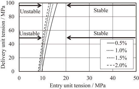
Figure 9 shows the numerical solution of eq. (24) obtained by using the experimental conditions in Table 1. Based on the calculation results of a discrete rolling model, the center deflection hr of the work-roll barrel was set to be
| \begin{equation*}
h_{r} = 9.92 \times 10^{-13}\ [\text{m/N}] \times P.
\end{equation*}
|
The true work-roll radius
R′ was calculated by Hitchcock’s equation.
11) The friction coefficient, etc. were set to empirical values. The vertical axis shows the delivery unit tension, and the horizontal axis shows the entry unit tension. The curves show the bifurcation curves. Lateral movement diverges (converges) in the left-side (right-side) region of these curves. The values in the legend show the reductions in thickness. The arrows show the stable and unstable regions of the experimental lateral movements. The calculation results in
Fig. 9 show that the critical entry unit tension in case of the delivery unit tension of 49 MPa and reduction of 1.5% is about 10.6 MPa, and the critical entry unit tension in case of the delivery unit tension of 98 MPa and reduction of 2.0% is about 12.6 MPa. Larger delivery tension increases the critical entry tension or causes lateral movement to become more unstable, but it seems that lateral movement does not depend significantly on the delivery tension under these experimental conditions. Comparing the calculation results in
Fig. 9 with the experimental results in
Figs. 7 and
8, it can be understood that the discriminant of
eq. (24) is accurate, thereby showing that the LMMs applied to formulating the discriminant are also accurate.
Figure 9 shows that smaller reduction decreases the stable region of lateral movement or causes lateral movement to become more unstable. The calculated value of the roll separating force (
P +
$P_{0}^{e}$ +
$P_{1}^{e}$) of 355 kN roughly agreed with the experimental value of 392 kN.
3.3 Clarification and consideration of lateral movement simulation
The lateral movement in experimental rolling is calculated by using the simulation built on MATLAB/Simulink. Figure 10 shows the simulation results of the lateral displacement at the mill in case of the delivery unit tension of 48 MPa. The horizontal axis and vertical axis show time and lateral displacement, respectively. A very small entry wedge of −0.45 µm was provided as the bias error so that the experimental results would agree with the simulation results. An entry unit tension of 22.05 MPa or more causes lateral movement to converge. On the other hand, the entry unit tension of under 17.15 MPa makes lateral movement diverge. Thus, the validity of the simulation is shown by the close agreement between the simulation results and the numerical results of eq. (24).
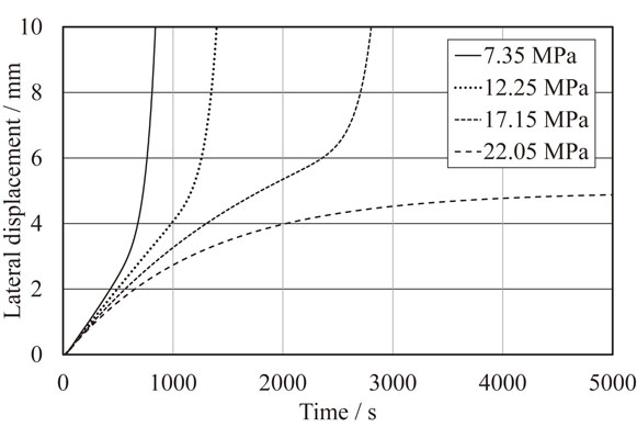
Figure 10 shows that the lateral displacement in case the entry unit tension of 7.35 MPa rapidly increases in about 700 s. Figure 11 shows the vertical deflections of the entry and delivery strips in 700 s. The z-axis shows the vertical direction. Out-of-plane deflection with torsion (lateral buckling) at the entry side of the mill, corresponding to Fig. 5, decreases the structural stiffness of a strip, and lower tension causes lateral buckling9) to occur more easily. On the other hand, the out-of-plane deflection at the delivery side of the mill in Fig. 11 does not appear, and also did not appear in the experiments.
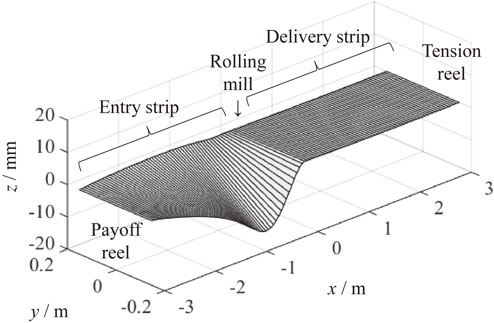
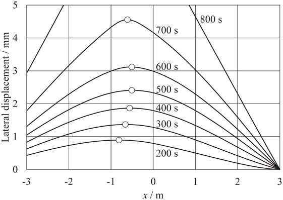
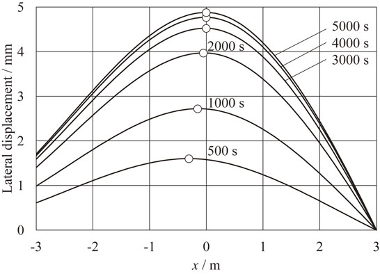
Figure 12 shows the simulation results of the lateral deflection in case of the entry unit tension of 22.05 MPa shown in Fig. 10. The horizontal axis shows the position in the strip rolling direction, and the vertical axis shows lateral displacement. With progressing time, lateral deflection converges in the steady state governed by eqs. (6), (13) and (17) of the boundary conditions. Lateral displacement shows its maximum at the mill entry side in the initial state of the calculation. Its maximum point approaches the mill in the steady state governed by eq. (6). Figure 13 shows the simulation results of the lateral deflection for the entry unit tension of 7.35 MPa in Fig. 10. In this case, lateral deflection diverges with progressing time. The point initially approaches the mill and departs from the mill after 600 s. The point appears at the mill entry side when lateral deflection diverges and entry tension is smaller than delivery tension. From eq. (1), the strip orientation angle at the mill becomes negative and the lateral movement velocity becomes positive in this case. Therefore, lateral movement continues to increase, and finally, lateral buckling occurs in the entry strip after 600 s.
The simulation results when the strip deflection model of the entry and delivery sides is a beam model constrained to in-plane deflection must agree with the discriminant of eq. (24). The broken curves in Fig. 14 show the simulation results of the lateral displacement at the mill when using a beam model. As in Fig. 10, the delivery tension is 49 MPa. The entry wedge, which is a bias error, is a relatively large value of −2.25 µm (that is, 5 times the value of −0.45 mm of the above-mentioned entry wedge, which is very small). The entry unit tensions of 9.8 MPa and 19.6 MPa cause lateral movement to diverge and converge, respectively. This linear dynamical system makes these results agree with the discriminant of eq. (24) regardless of the magnitude of bias errors.
The solid curves in Fig. 14 show the simulation results of the lateral displacement at the mill when using the large-deflection strip model. The solid curves agree with the broken curves in the initial term of the calculations, but the solid curves in the case of smaller entry tension gradually depart from the broken curves with progressing time.
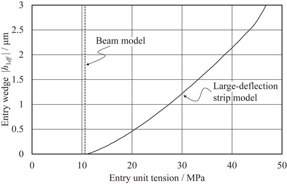
Figure 15 shows the phase diagram for the entry tension and the entry wedge based on the simulation results for reduction of 1.5%. The horizontal axis and vertical axis show the entry unit tension and the magnitude of the entry wedge, respectively. The solid curve and the broken line show the results obtained by using the large-deflection strip model and a beam model, respectively. The critical entry unit tension of 41.1 MPa obtained by using the large-deflection strip model is very different from the discriminant of eq. (24). Large values of the orientation angle θn or lateral displacement vn cause the lateral buckling in the entry strip to decrease the structural stiffness of the entry strip. Asymmetry error factors such as the entry wedge cause lateral movement. As mentioned above, this type of error cannot be ignored even if good operation is maintained in an actual temper rolling line. Applying the large-deflection strip model makes it possible to simulate lateral movement more safely. On the other hand, the discriminant of eq. (24) shows that asymmetry errors do not cause lateral movement, but the cause of lateral movement is an unstable dynamical system. Both a stable dynamical system and very small error make lateral movement converge. Facilities and operation must be managed in a stable condition for a dynamical system for lateral movement. It is considered that methods such as the discriminant of eq. (24) are valid as tools for a first-step study because these methods enable very simple calculation.
4. Conclusions
In this paper, the validity of lateral movement simulation was clarified by experimental rolling in the laboratory and a theoretical analysis with the aim of developing an automatic control system for the temper rolling line. The results obtained in this study are shown below.
-
(1)
A practical lateral movement simulator based on a newly-formulated LMM of a temper rolling and a strip deflection model were proposed.
-
(2)
The lateral movement in experimental rolling became excessive when the entry tension of the mill became smaller than a critical value. The mechanism of this behavior was clarified by the newly-formulated theoretical analysis (eigenvalue analysis) for evaluation of lateral movement.
-
(3)
It was confirmed that the experimental results within the range of experimental conditions in this study agreed with the simulation results, and the LMMs based on the quasi-static theoretical model were appropriate.
-
(4)
The newly-developed method provides the optimal rolling conditions for preventing lateral movement by theoretical analysis, calculations and experiments.
It is considered that the proposed methods can be applied generally to lateral movement analysis problems other than the temper rolling line and are useful for investigating lateral movement problems in further detail. However, the proposed strip deflection model is designed specifically for strips with camber and cannot be applied to strips with various defective shapes. Therefore, it will be necessary to design a more practical strip deflection model for these strips.
REFERENCES
- 1) M. Miyake, Y. Kimura, T. Kawai and T. Hiruta: Journees Siderurgiques International (The 30th JSI), (2012) pp. 59–60.
- 2) T. Ogasahara, T. Kitamura, S. Aoe, J. Tateno and K. Asano: Tetsu-to-Hagané 105 (2019) 512–521.
- 3) H. Matsumoto: J. JSTP 44 (2011) 237–242.
- 4) K. Nakajima, T. Kajiwara, T. Kikuma, T. Kimura, H. Matsumoto and M. Tagawa: Proc. 1980 Jpn. Spring Conf. Technol. Plast., (1980) pp. 61–64.
- 5) K. Nakajima, T. Kajiwara, T. Kikuma, T. Kimura, H. Matsumoto, M. Tagawa, I. Masuda and K. Yoshimoto: Proc. 31st Jpn. Jt. Conf. Technol. Plast., (1980) pp. 471–474.
- 6) H. Matsumoto and A. Ishii: Proc. 53th Jpn. Jt. Conf. Technol. Plast., (2002) pp. 117–118.
- 7) K. Komori: Tetsu-to-Hagané 104 (2018) 742–749.
- 8) S. Aoe, Y. Ohara, H. Hayashi and Y. Yoshinaga: Trans. Jpn. Soc. Mech. Eng. A 77 (2011) 1102–1111.
- 9) S. Aoe, Y. Ohara, M. Miyake and K. Kabeya: Tetsu-to-Hagané 104 (2018) 493–500.
- 10) S. Yanabe, S. Nagasawa and P. Mitsomwang: Trans. Jpn. Soc. Mech. Eng. 80 (2014) DSM0335.
- 11) H. Matsumoto: Theory and Practice of Flat Rolling (Revised edition), (ISIJ, Tokyo, 2010) pp. 33–42.
- 12) S. Aoe: Tokyo Tech. D.Eng. Thesis (2012) pp. A36–A45.
- 13) S. Yanagi, Y. Fujii, S. Koizumi and M. Kobayashi: CAMP-ISIJ 31 (2018) 724.
- 14) S. Aoe and M. Miyake: JP. 2018-118297 (2018).
- 15) S. Aoe, M. Miyake and K. Kabeya: CAMP-ISIJ 30 (2017) 502–503.
- 16) S. Nomura and S. Shintani: Theory and Practice of Flat Rolling (Revised edition), (ISIJ, Tokyo, 2010) pp. 240–242.
Appendix
A1 Formulation of eq. (2)
The strip rotational velocity ψ0 at the mill delivery side is defined as
| \begin{equation}
\psi_{0} = - \partial_{y}U
\end{equation}
| (A1-1) |
where
U is the strip velocity at the delivery side. Appling the definition of forward-slip
fs,
eq. (A1-1) is deformed to
| \begin{align}
\psi_{0}/U & = - (1 + f_{s})^{-1}\partial_{y}f_{s}\\
& = \beta_{h0}\frac{h_{0df}}{A} - \beta_{h1}\frac{(1 - r)h_{1df}}{A} + \beta_{M0}\frac{M_{0}}{kI} \\
&\quad - \beta_{M1}\frac{(1 - r)M_{1}}{kI}
\end{align}
| (A1-2) |
where
| \begin{equation}
\beta_{h0} = - h(1 + f_{s})^{-1}\partial_{h}f_{s},
\end{equation}
| (A1-3) |
| \begin{equation*}
\beta_{h1} = h(1 - r)^{-1}(1 + f_{s})^{-1}\partial_{h1}f_{s},
\end{equation*}
|
| \begin{equation}
\beta_{M0} = k(1 + f_{s})^{-1}\partial_{\sigma 0}f_{s},
\end{equation}
| (A1-4) |
| \begin{equation*}
\beta_{M1} = - k(1 + f_{s})^{-1}\partial_{\sigma 1}f_{s},
\end{equation*}
|
and
h1 are the thickness of the delivery and entry strip, and σ
0 and σ
1 are the delivery and entry unit tension. Appling the relationship between the entry and delivery wedges
16) and
eq. (A1-2), the strip rotational velocity ψ
1 at the entry side is represented by
| \begin{align}
\frac{\psi_{1}}{(1 - r)U} & = - (1 - \beta_{h0})\frac{h_{0df}}{A} + (1 - \beta_{h1})\frac{(1 - r)h_{1df}}{A}\\
&\quad + \beta_{M0}\frac{M_{0}}{kI} - \beta_{M1}\frac{(1 - r)M_{1}}{kI}.
\end{align}
| (A1-5) |
The entry rotational velocity ψ1 is also represented by3,6)
| \begin{equation}
D\theta_{n}/Dt = d\theta_{n}/dt + (1 - r)U\kappa_{1} = \psi_{1}
\end{equation}
| (A1-6) |
with the entry orientation angle θ
n. The following equation is formulated by substituting
eq. (A1-5) in
eq. (A1-6) and limiting strip reduction
r to zero:
| \begin{align}
\frac{d\theta_{n}}{dt} &= U\bigg\{- (1 - \beta_{h0})\frac{h_{0df}}{A} + (1 - \beta_{h1})\frac{h_{1df}}{A} \\
&\quad + \beta_{M0}\frac{M_{0}}{kI} - \beta_{M1}\frac{M_{1}}{kI} - \kappa_{1} \bigg\}.
\end{align}
| (A1-7) |
Substituting Bland & Ford’s forward-slip equation11) in eq. (A1-3), the influence coefficient βh0 is represented by
| \begin{align}
\beta_{h0} & =\Bigg( \frac{1}{2\sqrt{(1 - r)^{-1} - 1}} - \frac{\sqrt{\xi}}{2\mu}\\
&\quad + \frac{\sqrt{\xi}}{4\mu}\log \left(\frac{1}{1 - r}\left(\frac{k - \sigma_{0}}{k - \sigma_{1}} \right) \right) \Bigg)\\
&\quad \times \tan \bigg(\frac{1}{2}\mathop{\mathrm{atan}}\Big(\sqrt{(1 - r)^{-1} - 1}\Big) \\
&\quad - \frac{\sqrt{\xi}}{4\mu}\log \left(\frac{1}{1 - r}\left(\frac{k - \sigma_{0}}{k - \sigma_{1}} \right) \right) \bigg)
\end{align}
| (A1-8) |
where ξ is
h/
R′. Limiting reduction
r in
eq. (A1-8) to zero, the influence coefficient β
h0 is 1/4. The influence coefficient β
h1 is 1/4 in same operation.
Substituting Bland & Ford’s forward-slip equation11) in eq. (A1-4), the influence coefficient βM0 is represented by
| \begin{equation}
\beta_{M0} = \frac{k\sqrt{\xi}}{2\mu (k - \sigma_{0})}\tan \left(\frac{1}{2}\mathop{\mathrm{atan}}(\sqrt{r}) - \frac{\sqrt{\xi}}{4\mu}\log (r + 1) \right).
\end{equation}
| (A1-9) |
The following equation is formulated by expanding
eq. (A1-9) with respect to
$\sqrt{r} $:
| \begin{equation}
\beta_{M0} = \frac{k\sqrt{\xi}}{4\mu (k - \sigma_{0})}\sqrt{r} + o^{2}(\sqrt{r}).
\end{equation}
| (A1-10) |
Considering reduction
r to be negligible, the second term on the right side of
eq. (A1-10) is approximated as zero and the influence coefficient β
M0 is approximated as the first term on the right side. The influence coefficient β
M1 is also approximated similarly in operation. Substituting the approximation value 1/4 of the influence coefficient β
h0 and β
h1 in
eq. (A1-7),
eq. (2) is formulated.
A2 LMM and boundary conditions of payoff reel
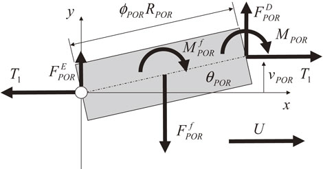
Figure A2-1 shows the force and moment acting on a strip that winds around a coil at a payoff reel. It is considered that the winding strip is developed to become a rigid body, and this rigid body moves on the developed plane of the coil. The surface of the rigid body moves from the left side to the right side. The entry endpoint (left endpoint) of the rigid body is fixed against the lateral direction, and the delivery endpoint (right endpoint) is connected with an elastic beam. The lateral friction force $F_{\textit{POR}}^{f}$
| \begin{equation}
F_{\textit{POR}}^{f} = - \frac{\phi_{\textit{POR}}\mu_{\textit{POR}}T_{1}}{\lambda_{\textit{POR}}U}\left(\frac{dv_{\textit{POR}}}{dt} + U\theta_{\textit{POR}} \right)
\end{equation}
| (A2-1) |
and the friction moment
$M_{\textit{POR}}^{f}$
| \begin{equation}
M_{\textit{POR}}^{f} = - \frac{\phi_{\textit{POR}}\mu_{\textit{POR}}T_{1}}{12\lambda_{\textit{POR}}U}(\phi_{\textit{POR}}^{2}R_{\textit{POR}}^{2} + b^{2})\frac{d\theta_{\textit{POR}}}{dt}
\end{equation}
| (A2-2) |
derived from rubbing between the surface of the rigid body and the plane of the coil act on the center of the rigid body.
14) In
eqs. (A2-1) and
(A2-2),
vPOR is the lateral displacement of the delivery endpoint of the rigid body, and θ
POR is the orientation angle of the rigid body. The relationship between the displacement
vPOR and the orientation angle θ
POR is formulated as follows:
| \begin{equation}
v_{\textit{POR}} = \phi_{\textit{POR}}R_{\textit{POR}}\theta_{\textit{POR}}.
\end{equation}
| (A2-3) |
The balance equation of moments is given by
| \begin{align}
&\phi_{\textit{POR}}R_{\textit{POR}}F_{\textit{POR}}^{f}/2 + M_{\textit{POR}}^{f} + \phi_{\textit{POR}}R_{\textit{POR}}F_{\textit{POR}}^{D}\\
&\quad - T_{1}v_{\textit{POR}} + M_{\textit{POR}} = 0
\end{align}
| (A2-4) |
where
$F_{\textit{POR}}^{D}$ and
MPOR are the lateral force and moment acting on the delivery endpoint of the rigid body.
Lateral force $F_{\textit{POR}}^{D}$ is represented by
| \begin{equation}
F_{\textit{POR}}^{D} = - (EI\partial_{xxx}v_{1}(- L) - T_{1}\partial_{x}v_{1}(- L))
\end{equation}
| (A2-5) |
by using the balance condition of the shear force of the elastic beam at the delivery endpoint. The connection conditions between the rigid body and the elastic beam are represented by
| \begin{equation}
\theta_{\textit{POP}} = \partial_{x}v_{1}(- L),\quad v_{\textit{POR}} = v_{1}(- L).
\end{equation}
| (A2-6) |
Considering
eqs. (A2-3) and
(A2-5) as the boundary conditions of the elastic beam and substituting the static equations shown as
eqs. (A2-1),
(A2-2),
(A2-5) and
(A2-6) in
eqs. (A2-3) and
(A2-4), the boundary conditions of
eqs. (12) and
(13) are formulated.