Metaheuristic Optimization of Powder Size Distribution in Powder Forming Process Using Multi-Particle Finite Element Method Coupled with Artificial Neural Network and Genetic Algorithm

Parviz Kahhal; Hossein Ghorbani-Menghari; Hwi-Jun Kim; Hyunjoo Choi; Pil-Ryung Cha; Ji Hoon Kim

doi:10.2320/matertrans.MT-MI2022006

Abstract

A neural network-based approach is proposed to minimize the maximum axial stress in the powder forming process. The finite element analysis was conducted using a MATLAB code and an ABAQUS python script to generate observations for the neural network training procedure. Powders of three different particle size distributions were mixed, and the mixture fractions were considered as control parameters. The artificial neural network determined the relationship between parameters and objective function. The effect of mixture fractions on maximum axial stress was analyzed. The results showed that the genetic algorithm could effectively determine the optima and the proposed method had strong prediction capability and accuracy.

1. Introduction

Powder compaction is an important technology in various industries and research fields. This technology combines various materials to fabricate materials with special properties. Powder compaction has a complicated procedure because of its complex nonlinear micromechanical deformation.¹^–³⁾ Zhang et al. investigated die compaction of copper powders with natural packing and vibrated packing using finite element and experimental methods.⁴⁾ They found a process condition that produces compacts with uniform and high relative density and stress distributions with the same pressure. Han et al. performed a multi-particle finite element method (MPFEM) for Fe and Al powders.⁵⁾ They utilized the discrete element method (DEM) to generate the initial packing structure used in the finite element model. They investigated the influence of Al powder on the deformation of particles, relative density and stress and distribution, and pressure. With the same compaction pressure, they found that the relative density increased when the Al powder increased. When the load is released, the internal stress sharply decreases near the surface zone. Abdelmoula et al. used MPFEM to investigate the plastic flow of a granular material.⁶⁾ The effect of stress on plastic strain along two loading paths up was studied. They found that the numerical models behave well based on a flow law, except near the loading region, where the effect of stress increment is very significant. Lei et al. carried out the densification behaviors of powder particles through powder compaction with the finite element method.⁷⁾ They considered several initial packing densities, including random, tetragonal, and hexagonal configurations. They evaluated the influence of friction, the size of particles, and the velocity of compaction on the compaction density. They utilized a response surface method to optimize the compaction process. Korim et al. investigated single-die compaction of solid copper powder and spongy powder using a two-dimensional MPFEM.⁸⁾ They studied the influence of external pressure and initial packing density on densification. They found that the densification of the sponge powder at low and medium relative density is faster than the solid powder. Demirtas et al. investigated the compaction of hollow spheres experimentally and numerically.⁹⁾ They found that the effect of the particle diameter on shell-thickness (d/w) is significant in the powder compaction. Van der Haven et al. carried out a powder compaction finite element analysis using the density-dependent Drucker-Prager Cap model to improve the pharmaceutical tablets design process.¹⁰⁾ They proposed a mixing methodology to determine mixture parameters. Zhou et al. compared the accuracy of 2D and 3D MPFEM in predicting the densification behavior.¹¹⁾ They considered a Ti–6Al–4V powder under various impact energy. They found 3D multi-particle finite element method produced a more accurate prediction than the 2D.¹¹⁾ Kahhal et al. developed an ABAQUS python script to generate MPFEM models to analyze the deformation of the particles in compaction.¹²⁾ The effects of loading path, configuration, and wall friction on punch force, stresses, and strains were analyzed.

Keshavarz et al. developed a genetic optimization algorithm to reduce defects during hot powder compaction.¹³⁾ The numerical simulation of the powder compaction was carried out using a temperature-dependent modified cap plasticity model. Hussain et al. investigated the impact of various powder process parameters (milling time, compaction pressure, sintering temperature, and holding time) on the density and hardness of Al₂O₃/Cu composites using the Taguchi method and Grey relational analysis.¹⁴⁾ They found an optimum parameter set and concluded that the density is more susceptible than the hardness for the given process parameters.

Tamura et al. investigated the impact of machine learning (ML)-driven optimization on gas atomization process parameters for producing Ni–Co based superalloy powders for turbine-disk applications.¹⁵⁾ By utilizing Bayesian optimization without expert assistance and starting with a small dataset, they determined the optimal melt temperature and gas pressure through three optimization cycles. Ladani et al. explored the potential synergy between artificial intelligence (AI) and additive manufacturing (AM).¹⁶⁾ Data types, sources, variabilities in experimental and simulation data, and their suitability for ML algorithms were investigated.

In this study, we present a novel approach to address the challenge of minimizing the maximum axial stress in the powder-forming process through the utilization of artificial neural networks (ANN). While previous research has investigated the effect of size distribution on powder compaction, our work advances the field by introducing an innovative combination of finite element analysis, ANN modeling, and optimization techniques. Unlike traditional approaches that rely solely on numerical simulations, we leverage the power of ANN to establish a comprehensive understanding of the relationship between control parameters, such as mixture fractions, and the objective function of minimizing maximum axial stress. By employing a representative volume generation method and a carefully designed ANN architecture, our approach effectively captures the complex behavior of the powder-forming process, enabling accurate predictions and efficient optimization. Through extensive experimentation on mixtures of Fe-based powders with three different size distributions, our results demonstrate the proposed method’s effectiveness and shed light on the interplay between mixture fractions and maximum axial stress. The integration of ANN modeling and optimization techniques showcases the potential for advancements in powder-forming processes and lays the foundation for future research and optimization efforts in the field.

2. Methods

2.1 Material properties

The compaction of Fe–Si–Al–P alloy powder was analyzed using the elasto-plastic material model. The material properties of this model are presented in Table 1. The compaction test was conducted using the Instron 8501 Servo Hydraulic Machine. This machine employs a servo-controlled hydraulic system to apply compressive loads on the samples. The maximum pressure applied throughout the experiment was maintained at 1.2 GPa. Furthermore, the compression test was performed for samples sintered at the temperature of 950°C. The utilization of the power law swift hardening method allowed for the extrapolation of the experimental compression data and determination of the stress-strain curve (see Fig. 1). The following equation depicts the flow stress-plastic strain relationship for this material:

\begin{equation} \sigma\ (\text{MPa}) = 1380(\varepsilon + 0.0354)^{0.254} \end{equation}

(1)

Table 1 Material parameters of Fe–Si–Al–P alloy powder.

Fig. 1

Stress-strain curve of the Fe–Si–Al–P alloy powder.

2.2 Powder size distribution

Three powders with different size distributions were studied in this work, as shown in Fig. 2. The powders with particle size in the ranges of 45–63 µm, 90–150 µm, and 150–300 µm were denoted as Powder 1, Powder 2, and Powder 3. The mixtures of various weight fractions of the three powders were studied. For example, the [50, 30, 20] mixture stands for a mixture with the fractions of 50%, 30%, and 20% for Powder 1 (m₁), Powder 2 (m₂), and Powder 3 (m₃), respectively.

Fig. 2

Particle size distributions of the three powders.

2.3 Representative volume element generation

To generate Representative Volume Elements (RVEs), the necessary number of particles was created while considering factors such as weight fraction, initial relative density, and avoiding particle overclosure. For this purpose, a MATLAB code from a previous study¹²⁾ was employed, which had been developed specifically for this task. The input parameters utilized for generating the RVEs are detailed in Table 2.

Table 2 Input parameters of the RVE generation.

2.4 Finite element model

The generated Representative Volume Elements (RVEs) were employed to construct ABAQUS finite element models using a Python script. The outcomes of the generated RVEs used for Finite Element Method (FEM) for four distinct mixture configurations are presented in Table 3. Figure 3 shows the arrangement of the generated RVEs for four mixture configurations. Additionally, Fig. 4 illustrates the axial stress-relative density curves for these four different powder mixtures. Table 4 summarizes the parameters of the finite element model.

Table 3 Properties of RVEs of four different powder fractions.

Fig. 3

Initial RVE configurations of the mixtures of four different fractions: (a) [100, 0, 0], (b) [0, 100, 0], (c) [0, 0, 100], and (d) [33, 33, 33].

Fig. 4

The axial stress-relative density curves of the four powder mixtures with different fractions.

Table 4 Parameters of the finite element model.

2.5 Optimization problem

Minimizing the maximum axial stress based on the effect of mixture fraction is the goal of optimization. So the optimization problem can be represented in the following form:¹⁷⁾

\begin{equation} \text{Minimise}\ F(M) = \textit{Obj}_{s}\ (m_{1},m_{2},m_{3}) \end{equation}

(2)

Subject to:

\begin{align*} &0 \leq m_{1} \leq 100\\ &0 \leq m_{2} \leq 100\\ &0 \leq m_{3} \leq 100 \end{align*}

Constraint:

\begin{equation*} m_{1} + m_{2} + m_{3} = 100 \end{equation*}

where m₁, m₂, m₃ are the volume fractions (%) of three powders, and F(M) is the minimum axial stress as a Obj_s of the determined optimizations at the relative density of 90%.

2.5.1 Artificial neural networks

The multilayer perceptron (MLP) is a type of artificial neural network (ANN) that follows a feed-forward architecture. It comprises multiple layers of interconnected neural cells. Each neuron in a layer is linked to the neurons in adjacent layers. The input values are provided to the first layer, while the output is computed in the final layer. The hidden layers reside between these input and output layers.¹⁶^,¹⁸⁾ The connections between neurons are represented by weights, and the MLP is trained by adjusting these weights to ensure that the computed outputs align with the desired predictions. Figure 5 depicts a schematic of the MLP structure and its neurons.

Fig. 5

Schematic of MLP and neurons.

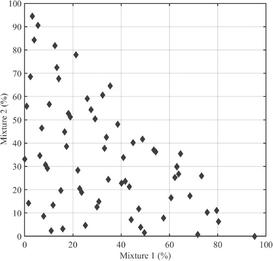
For the purpose of this study, a space-filling Latin hypercube sampling design was employed to generate 65 observation points for the design of experiments (DOE). Figure 6 displays the pairwise projections of the variables in the study.

Fig. 6

Pairwise projections of the process variables.

2.5.2 Genetic algorithm

The genetic algorithm (GA) is a technique that mimics the natural processes in ecosystems.¹⁹⁾ It is a well-known optimization method used to solve complex problems. The GA flowchart, illustrated in Fig. 7, is a widely used framework that involves the creation of an initial population of potential solutions, the evaluation of the fitness of each solution, and the selection of the fittest individuals to reproduce and generate offspring through crossover and mutation operations. The genetic algorithm follows the following steps:

1. Initialization: A population P is created with randomly generated real values, forming a set of possible solutions.
2. Evaluation: A fitness function is applied to assess the fitness of each chromosome in the population by calculating g(P).
3. Selection: Chromosomes are ranked based on their fitness values, and parents are chosen for crossover and mutation based on this ranking.
4. Genetic operators: New offspring or chromosomes (C₁, C₂) are generated from the selected parents and added to the children population; C.
5. Crossover: Information is exchanged between the two parents.
6. Mutation: The genes of the offspring chromosomes resulting from crossover undergo mutation, introducing changes.

The aforementioned steps are repeated in an iterative manner until a termination condition is satisfied. This condition may involve reaching a predetermined maximum number of iterations or attaining the desired fitness value.

Fig. 7

GA flowchart.

3. Results and Discussion

3.1 Artificial neural networks

The available observations of Cases 1, 2, 3, and 4 were utilized to train an Artificial Neural Network (ANN) for the objective function. The optimal number of neurons and layers were determined using a grid search approach. Multiple parameter combinations were tested, and the combination that yielded the most favorable outcomes was identified. The selection of the best combination was based on minimizing the standard deviation of the residuals (RMSE) across the training (70%), testing (15%), and validation (15%) data sets. The Table 5 provides the detailed parameters of the trained ANN.

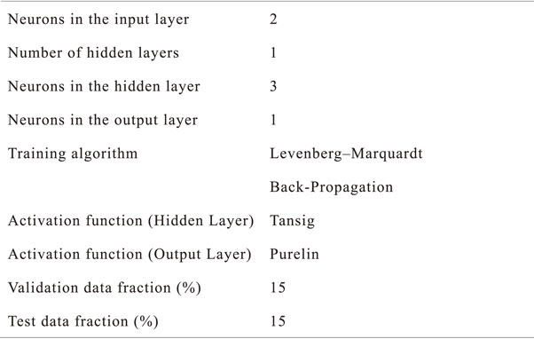
Table 5 Parameters of the trained ANN.

To ensure optimal predictive capability without encountering underfitting or overfitting, the number of neurons and layers in the Artificial Neural Network (ANN) were meticulously chosen.

Table 6 provides an overview of the statistical characteristics of the trained ANN, encompassing the Mean Squared Error (MSE), Root Mean Squared Error (RMSE), and the correlation coefficient (R). The MSE value of 20.9188 signifies the average squared difference between the predicted and actual values, with a lower value indicating a stronger alignment.

Table 6 Statistical features of the trained ANN.

The RMSE value of 4.5737 represents the standard deviation of the residuals, reflecting the ANN’s accuracy, where a smaller value implies higher precision. The correlation coefficient (R) of 0.96737 reveals a strong positive correlation between predicted and actual values, suggesting close alignment with the observed data. Overall, these statistical features highlight the ANN’s strong predictive capability for the given objective function, as evidenced by its low MSE and RMSE, and high correlation coefficient (R).

Figure 8 depicts the predicted surface of axial stress at a relative density of 90% for the independent design variables, m₁ and m₂. It provides insights into the relationship between these variables and the resulting axial stress.

Fig. 8

ANN predicted surface of the Axial stress objective based on the independent design variables, m₁ (Mixture 1) and m₂ (Mixture 2).

Figure 9 displays diagrams comparing predicted and observed values for different datasets: (a) training (R = 0.96737), (b) validation (R = 0.96745), (c) test (R = 0.97606), and (d) all datasets combined (R = 0.96631). These diagrams demonstrate the model’s ability to closely align predicted values with observed values across various datasets. The high correlation coefficients indicate strong predictive performance, with the test dataset showing the highest correlation. Combining all datasets yields a good overall fit, as indicated by the correlation coefficient of 0.96631. The observation values of the objective function are represented as targets in the horizontal axis, while the predicted output of the ANN for the corresponding inputs is represented as outputs in the vertical axis. The ideal scenario is when all the points fall on the diagonal line, indicating perfect prediction. A high accuracy model would have points closely clustered around this diagonal line, indicating a strong alignment between predicted and observed values.

Fig. 9

Diagrams showing predicted versus observed values for datasets: (a) training, (b) validation, (c) test, and (d) all datasets.

3.2 Optimization result

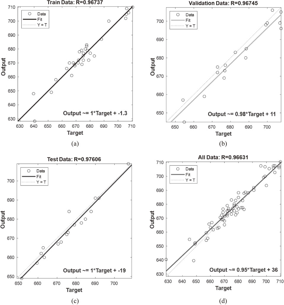
Table 7 summarizes the optimization results. It includes the best variable configuration and the corresponding predicted and analyzed values for the objective of axial stress. The variables m₁, m₂, and m₃ are expressed as percentages, with optimized values of 25.02%, 5.52%, and 69.45% respectively. The predicted axial stress is 640.4 MPa, while the analyzed axial stress is 639.0 MPa. The small difference of less than 1% between the predicted axial stress and the analyzed axial stress highlights the high predictability of the trained ANN. This suggests that the ANN model can accurately estimate the axial stress, as the predicted values closely align with the analyzed values. Figure 10 shows the von Mises stress distribution of the optimum mixture during compaction.

Table 7 The optimization results.

Fig. 10

Von Mises stress distribution of the optimum mixture during compaction.

Figure 11 illustrates the axial stress-relative density curves of the optimized mixture and three pure powders (Powder 1, Powder 2, and Powder 3) with their corresponding percentages of [m₁, m₂, m₃]. The optimized mixture has the axial stress at the relative density of 90% value of 639.0 MPa, while Powders 1, 2, and 3 has the axial stress of 722.4 MPa, 698.2 MPa, and 708.9 MPa, respectively. These results show that the optimized mixture has the lowest axial stress value compared to the other mixtures. This indicates that the optimized mixture may be the most effective for the desired application, as it achieves the desired stress performance while maintaining a relatively high density level.

Fig. 11

Relative density (%)-axial stress curves for the optimum mixture and the three pure powders.

Figure 12 depicts the evolution of particle shape and stress during different stages of the compaction process. The figure illustrates that small particles were distributed evenly between large particles, filling the voids. Physical connections between the small and large particles create interparticle bridging, allowing this filling. The powder mixture became more tightly packed during the compaction process as small particles were compacted between larger particles through the interparticle bridging. This increased density can enhance the material properties of the final product, such as strength, stiffness, and wear resistance.

Fig. 12

Evolution of particle shape and stress during different stages of the compaction process.

4. Conclusion

A multi-particle finite element simulation of the powder compaction process was conducted to investigate the effect of the powder size distributions. Modules of FE mesh generation, FE calculation, and postprocessing were utilized. An ANN was trained using grid search-based hyper-tuning to prevent overfitting and underfitting. A genetic algorithm was used to find the optimum powder-size mixture with minimum axial stress or maximum density. The following conclusions were drawn:

(1) The MATLAB based particle generator and ABAQUS python script combine to generate powder compaction data of various powder size distributions for ANN training.
(2) The combination of the ANN and the genetic algorithm successfully determined the optimum powder size distribution for minimizing axial stress for a given relative density at a low computational cost.

The neural network-based optimization approach proposed in this research offers opportunities for process optimization, material design, predictive modeling, model refinement, and integration with process control systems. The findings and methodology can serve as a foundation for further research and development in the field of powder forming, contributing to enhanced manufacturing processes and product quality.

Acknowledgments

This work was supported by the National Research Foundation of Korea (NRF) Grant funded by the Korean Government (MSIP) (No. Grant Number – NRF-2021M3H4A6A01045764).

REFERENCES

Corresponding author

Register with J-STAGE for free!

REFERENCES

- 1) A. Baroutaji, K. Bryan, M. Sajjia and S. Lenihan: Mechanics and Computational Modeling of Pharmaceutical Tabletting Process, Reference Module in Materials Science and Materials Engineering, (Elsevier, Amsterdam, 2017).
- 2) S. Inghelbrecht and J.P. Remon: Int. J. Pharm. 161 (1998) 215–224. doi:10.1016/S0378-5173(97)00356-6
- 3) C.Y. Wu, O.M. Ruddy, A.C. Bentham, B.C. Hancock, S.M. Best and J.A. Elliott: Powder Technol. 152 (2005) 107–117. doi:10.1016/j.powtec.2005.01.010
- 4) X. An, Y. Zhang, Y. Zhang and S. Yang: Metall. Mater. Trans. A 46 (2015) 3744–3752. doi:10.1007/s11661-015-2929-x
- 5) P. Han, X. An, Y. Zhang, F. Huang, T. Yang, H. Fu, X. Yang and Z. Zou: Powder Technol. 314 (2017) 69–77. doi:10.1016/j.powtec.2016.11.021
- 6) N. Abdelmoula, B. Harthong, D. Imbault and P. Dorémus: J. Mech. Phys. Solids 109 (2017) 142–159. doi:10.1016/j.jmps.2017.07.021
- 7) Y. Lei, S.W. Yan, S.Y. Huang, W. Liu, S.M. Sun, M.C. Zhou and F. Feng: J. Adv. Mech. Des. Syst. Manuf. 12 (2018) JAMDSM0022. doi:10.1299/jamdsm.2018jamdsm0022
- 8) N. Korim and L. Hu: Mater. Res. Express 7 (2020) 056509. doi:10.1088/2053-1591/ab8cf6
- 9) A. Demirtas and G. Klinzing: Powder Technol. 391 (2021) 34–45. doi:10.1016/j.powtec.2021.06.004
- 10) D.L.H. van der Haven, F.H. Ørtoft, K. Naelapää, I.S. Fragkopoulos and J.A. Elliott: Powder Technol. 403 (2022) 117381. doi:10.1016/j.powtec.2022.117381
- 11) J. Zhou, H. Xu, C. Zhu, B. Wang and K. Liu: Arch. Metall. Mater. 67 (2022) 57–65. doi:10.24425/amm.2022.137472
- 12) P. Kahhal, J. Jung, H. Choi, P.R. Cha and J.H. Kim: Mater. Trans. 63 (2022) 1576–1582. doi:10.2320/matertrans.MT-MB2022012
- 13) S. Keshavarz, A.R. Khoei and Z. Molaeinia: Int. J. Adv. Manuf. Technol. 64 (2013) 1057–1072. doi:10.1007/s00170-012-4053-z
- 14) M.Z. Hussain, S. Khan and P. Sarmah: J. King Saud Univ. Eng. Sci. 32 (2020) 274–286. doi:10.1016/j.jksues.2019.01.003
- 15) R. Tamura, T. Osada, K. Minagawa, T. Kohata, M. Hirosawa, K. Tsuda and K. Kawagishi: Mater. Des. 198 (2021) 109290. doi:10.1016/j.matdes.2020.109290
- 16) L.J. Ladani: J. Phys. Mater. 4 (2021) 042009. doi:10.1088/2515-7639/ac2791
- 17) P. Kahhal, M. Ghasemi, M. Kashfi, H. Ghorbani-Menghari and J.H. Kim: Sci. Rep. 12 (2022) 2837. doi:10.1038/s41598-022-06652-3
- 18) P. Kahhal, J. Jung, Y.C. Hur, Y.H. Moon and J.H. Kim: Materials 15 (2022) 1430. doi:10.3390/ma15041430
- 19) P. Kahhal, S.Y. Ahmadi-Brooghani and H.D. Azodi: J. Mech. Sci. Technol. 27 (2013) 3835–3842. doi:10.1007/s12206-013-0927-8