Mechanics of Materials
Towards Predicting Necking Instability in Metals by Acoustic Emission Model Analysis
2024 Volume 65 Issue 3 Pages 292-301

Details
2024 Volume 65 Issue 3 Pages 292-301
We have enhanced a basic single-variable dislocation evolution modelling framework to encompass the acoustic emission (AE) characteristics observed in metals and alloys during the homogeneous strain hardening stage up to the point of macroscopic necking instability under tensile stress. To validate our proposed modelling approach, we conducted comprehensive experiments using pure Ag, Cu, Al, and Ni, representing fcc metals with stacking fault energies increasing in the listed order of materials. Our model successfully captures both previously established and newly discovered patterns in the evolution of the AE spectral density. A key focus of this research is to demonstrate the ability to directly derive the critical parameter that governs the evolution of dislocations and, consequently, overall strain hardening, namely the rate of dynamic dislocation recovery, directly from AE measurements. As a prime result, we can predict the conditions leading to necking, specifically the necking strain, well in advance solely from AE data.

Acoustic Emission (AE) is widely known as a release of transient elastic waves from local sources associated with rapid stress relaxation in a material under load. AE accompanies many irreversible processes occurring in plastically deforming solids, including dislocation motion, mechanical twinning, stress- or strain-induced phase transformations and cracking.1–8) The AE technique has been recognised to be highly sensitive to dislocation dynamics since the very first work by J. Kaiser (dated back to 19509)) followed by Fisher and Lally10) who were the first to relate the AE bursts to the intermittent dislocation motion. Then Tetelman, Gillis, Pollock, James and Carpenter, Mallen and Bolin, Ono, Kishi et al.3,11–19) pioneered the fundamental studies on the AE behaviour in plastically deforming metals and engineering alloys, circa in 1970s. Nonetheless, despite a long history, the method has received a large portion of criticism for its complex indirect relation with the source and the descriptive character, providing primarily qualitative information to researchers, which is not always sufficient for decision-making when features of plastic deformation and its transition to cracking are of concern. This bleak picture has set a tone on the research community and in the minds of practitioners who often believe that reliable forecasting of imminent failure is not possible with the AE data. In this study, we outline a selection of captivating outcomes from our recent endeavours to rectify the just stated existing issue and tackle the underlying core limitation within the AE method. This major limitation revolving around the absence of a predictive AE methodology stems from the lack of an adequate microstructurally-informed model of the AE behaviour in solids under load. We aim to demonstrate that, relying on the well-established principles of strain hardening theory, it is fundamentally feasible to transform the modern AE method into a powerful quantitative laboratory tool. This tool can be tailored for the analysis of dislocation evolution and is well-suited for predicting macroscopic plastic instabilities of the necking type.
Commercial purity metals - silver, copper, aluminium, and nickel distributed by Nilaco Corporation (Japan), were used in the present study. Ag, Cu and Al are nominally of 4N purity, and Ni is of 3N grade. Having an fcc lattice, the chosen materials are vastly different in their stacking fault energy (SFE) controlling the dislocation mobility. The SFE value χSFE varies in ascending order from 18–25 mJ/m2 for Ag, and 40–70 mJ/m2 for Cu, to 170–250 mJ/m2 for Al and ∼300 mJ/m2 for Ni.20–23) The flat dog-bone-shaped specimens with a gauge length of 15 × 7 × 2 mm3 were cut by an electric discharge machine. They were annealed in vacuum for 90 minutes at 0.85Tm (Tm is melting temperature) prior to testing. The grain size was measured by the electron back-scattered diffraction technique using the field emission scanning electron microscope (SEM) Zeiss SIGMA.
Uniaxial tensile testing was carried out using a screw-driven Tinius Olsen H50KT machine with a 5 kN load cell and a clip-on extensometer with 1 µm resolution. The constant cross-head speed corresponded to a nominal strain rate of 2 × 10⁻³ s−1.
The acoustic emission signal was recorded by a wideband piezoelectric transducer NF AE-900S-WB (Japan), which has a nominal frequency band from 100 to 900 kHz. The signal was amplified by 60 dB by a low noise PAC 2/4/6 amplifier and acquired digitally by the PCI-2 board (Physical Acoustic Corporation, USA). The thresholdless streaming waveform recording was implemented at the sampling rate of 2 Msamples/s, thus satisfying the Nyquist criterion for aliasing-free reconstruction of the signal from a sampled dataset. Silicone vacuum grease was used as a coupling medium to ensure efficient wave transfer from the surface to the transducer.
The continuously streamed data were sectioned into consecutive individual realisations of 4096 samples. For each realisation, a power spectral density (PSD) function G(f) was calculated using a Welch method implemented in the adaptive sequential k-means (ASK) data clustering and analysis algorithm.24) The AE power and the spectral median frequency are introduced as primary PSD descriptive variables according to the following equations:
| \begin{equation} P_{\text{AE}} = \int_{0}^{\infty}G(f)df \end{equation} | (1) |
| \begin{equation} \int_{0}^{f_{\text{m}}}G(f)df = \int_{f_{\text{m}}}^{\infty}G(f)df \end{equation} | (2) |
Both PAE and fm were obtained from G(f) after subtraction of the PSD of the laboratory noise pre-recorded before the start of loading during each test. Details of specific AE signal processing algorithms applied in the present work are documented in Refs. 25–27). Reasons are also provided in the cited works for the choice of PAE and fm as primary physically significant variables, which are used to characterise each realisation of the AE random process. Some of these reasons will be briefly reiterated below.
The proposed approach is grounded on the following three premises. 1) The raw AE signal U(t) at the sensor output is represented by a continuous random Ornstein-Uhlenbeck like process satisfying the stochastic differential equation:
| \begin{equation} \frac{dU}{dt} = -\frac{U}{\tau_{r}} + \tilde{\xi}(t) \end{equation} | (3) |
where $\tilde{\xi }(t)$ represents the white Gaussian noise, which captures the stochastic nature of the dislocation behaviour arising from thermally activated dislocation “birth” processes (e.g., breaking away from pinning points, nucleation at grain boundaries or at a free surface), navigating through a collection of randomly distributed obstacles, and the probabilistic process of dislocation annihilation of a general kind; τr denotes the intrinsic relaxation time within a collection of sources, acting as a comprehensive and fundamental indicator of the temporal interrelation among individual occurrences within the time series. 2) The total density of dislocations ρ is an intrinsic microstructural state variable governing the macro-mechanical response in terms of extrinsic stress σ and strain ε, which cannot be regarded as state variables. The population of dislocations evolves in line with first-order kinetics laws accounting for the ‘birth and death’ of dislocations through a differential equation having a general structure combining the rates of dislocation generation $\frac{d\rho^{ + }}{d\varepsilon }$ and annihilation $\frac{d\rho^{ - }}{d\varepsilon }$ with strain as
| \begin{equation} \frac{d\rho}{d\varepsilon} = \frac{d\rho^{+}}{d\varepsilon} - \frac{d\rho^{-}}{d\varepsilon} \end{equation} | (4) |
The exact form of this equation can vary significantly, depending on the dislocation reactions involved in the production and disappearance of dislocations. Its simplest form has been proposed by Kocks and Mecking28,29) (see also related earlier works by Bergstrom30) and Klepaczko31))
| \begin{equation} \frac{d\rho}{d\gamma} = \frac{d\rho}{Md\varepsilon} = \frac{k_{1}}{b}\sqrt{\rho} - k_{2}\rho \end{equation} | (5) |
Here k1 and k2 are dimensionless constant parameters that govern the evolution of the dislocation density by controlling the rates of dislocation production and dynamic recovery, respectively. The coefficient k1 is supposed to be athermal, while the coefficient $k_{2}(\dot{\varepsilon },T)$ depends on the strain rate and temperature to account for the thermally activated recovery processes. 3) The flow stress is related to the total dislocation density by the Taylor equation in the form:
| \begin{equation} \sigma(\varepsilon) = M\tau(\gamma) = M\alpha \mu b\sqrt{\rho(\gamma)} \end{equation} | (6) |
where M stands for the texture-related orientation factor that transforms shear stress τ and strain γ to corresponding axial parameters as τ = σ/M, γ = εM; b is the magnitude of the Burgers vector of the dislocation, μ is the shear modulus, and $\alpha = \alpha (\dot{\varepsilon },T)$ is a numerical factor ranging typically between 0.1 and 0.5 depending on the dislocation arrangement, strain rate and temperature.32) The strong reliance of this arrangement on the dislocation mobility suggests a potential connection of α to the stacking fault energy χSFE,33) although the precise nature of the α(χSFE) relationship remains uncertain in its explicit form. To maintain simplicity, we omitted the consideration of frictional stress in eq. (6), a choice typically justifiable for fcc metals and alloys. Combining eqs. (5) and (6), and solving the initial value problem (with σ(ε = 0) = σ0) for the flow stress σ(ε), one simply obtains the familiar stress-strain relation:
| \begin{equation} \sigma(\varepsilon) = \sigma_{0} + (\sigma_{S} - \sigma _{0})\left(1 - \exp\left(-\frac{\varepsilon}{\tilde{\varepsilon}}\right)\right) \end{equation} | (7) |
The introduced here constant parameters σS and $\tilde{\varepsilon }$ are defined as:
| \begin{equation} \sigma_{S} = \frac{k_{1}M\alpha\mu}{k_{2}},\quad \tilde{\varepsilon} = \frac{2}{k_{2}M} \end{equation} | (8) |
The value of σS corresponds to the so-called saturation stress that obeys the condition $\frac{d\sigma }{d\varepsilon } = 0$, and $\tilde{\varepsilon }$ is the parameter directly related to the necking strain,34–36) as will be discussed below.
The strain hardening rate $\theta (\varepsilon ) = \frac{d\sigma (\varepsilon )}{d\varepsilon }$ is obtained from eq. (7) as follows:
| \begin{equation} \theta(\varepsilon) = \frac{1}{\tilde{\varepsilon}}(\sigma_{S} - \sigma_{0})\exp \left(-\frac{\varepsilon}{\tilde{\varepsilon}}\right) = \frac{1}{\tilde{\varepsilon}}(\sigma_{S} - \sigma(\varepsilon)) \end{equation} | (9) |
AE sources, which are associated with the transformation in the microstructure due to the motion and annihilation of mobile dislocations, appear to be inherently linked to the above fundamental solutions. The experimentally obtained AE parameters, such as AE power and the median frequency of the spectral density, can be linked to the development of the defect microstructure under increasing load. Drawing inspiration from the concepts articulated by the AE pioneers in the 70th of the past century,2,3,11,16,37,38) we treat AE as a result of fluctuating intermittent dislocation motion, generating the continuous random Ornstein-Uhlenbeck process in accordance with eq. (3).39–41) Stochastic properties of this process are well documented; notably, its power spectral density is given by a familiar Lorentz-type function:42,43)
| \begin{equation} G(f) = 4\sigma_{\text{UU}}^{2}\frac{f_{\text{c}}}{f_{\text{c}}^{2} + 4\pi^{2}f^{2}} \sim P_{\text{AE}}\frac{f_{\text{c}}}{f_{\text{c}}^{2} + 4\pi^{2}f^{2}} \end{equation} | (10) |
where $\sigma_{\text{UU}}^{2}$ is the variance of the AE signal, serving as a measure of the power of the random AE process, and fc = 1/τr, in this context, is a characteristic frequency that determines the effective width of the power spectrum. The fc value decreases with the increasing relaxation time τr; consequently, the spectrum shifts to lower frequencies and vice versa. Using the definition of the median frequency fm, eq. (2), for the spectrum defined by eq. (10), it appears that fc is the median frequency of the spectrum (10) to a factor of 2π: fc = 2πfm.25) For precisely this rationale, out of numerous possible frequency characteristics for the AE PSD, we have selected the median frequency to complement the power, with the note that both attributes independently contribute to eq. (10). The relaxation time τr can be related to the dislocation mean free path ⟨Λ⟩ and the average dislocation velocity ⟨V⟩ as:40)
| \begin{equation} \tau_{\text{r}} = \langle \Lambda \rangle/\langle V \rangle \end{equation} | (11) |
Using Orowan’s expression for the plastic strain rate
| \begin{equation} \dot{\varepsilon} = M\rho_{\text{m}}b\langle V \rangle \end{equation} | (12) |
(here ρm symbolises the mobile dislocation density), Taylor eq. (6), and recalling that ⟨Λ⟩ scales with the dislocation density as $\langle \Lambda \rangle \sim 1/\sqrt{\rho } $44) in nearly all imaginable dislocation arrangements that arise during monotonic tensile plastic deformation, it can be concluded that the AE median frequency is directly proportional to the square root of the total dislocation density, while inversely correlated with the density of mobile dislocations as:
| \begin{equation} f_{\text{m}} \sim \frac{M\dot{\varepsilon}}{b\rho_{\text{m}}}\sqrt{\rho} = K_{\text{f}}\frac{\dot{\varepsilon}}{\rho_{\text{m}}}\sigma \end{equation} | (13) |
Here, the factor Kf consolidates all constants derived from the respective eqs. (6) and (12). It also effectively accounts for the AE transfer function, albeit in an indirect way. Thus, the model predicts that during homogeneous plastic deformation, the AE median frequency fm scales linearly with the flow stress $f_{\text{m}} \sim \sqrt{\rho } \sim \sigma $ and strain rate $f_{m} \sim \dot{\varepsilon }$.
Considering the average elastic energy dissipated per unit time due to the elementary displacement of dislocation segments driven by a Peach-Köhler force through a crystalline lattice, we derived the expression for the AE power39) in the following form
| \begin{equation} P_{\text{AE}} = K_{\text{AE}}\rho_{\text{m}}\frac{\theta}{\sigma}\dot{\varepsilon} = K_{\text{AE}}\rho_{\text{m}}\frac{\dot{\sigma}}{\sigma} \end{equation} | (14) |
that explicitly correlates PAE with strain hardening and the mobile dislocation density. A linear relationship is thus anticipated between the experimentally measured AE power PAE and the reduced hardening rate $\dot{\sigma }/\sigma $, provided ρm does not vary significantly during the uniform deformation stage. The factor KAE, similarly to Kf, integrates all relevant model parameters into a single proportionality constant.
Typical fragments of AE realisations of 1 s duration acquired from the materials tested at about 5–7% plastic strain are shown in Fig. 1. In a precise sense, the AE signal undergoes changes over time and strain and cannot be considered a “perfectly” stationary stochastic process. Nonetheless, it exhibits a quasi-stationary behaviour within the time frame of individual realisations. The signal fluctuations occur on a much shorter timescale than the duration of a single AE “frame” (4096 readings equal to ∼2 ms) used in data processing, and the changes in the overall signal occur much slower than it can be noticed in individual AE realisations.

Randomly picked typical fragments of continuous AE wav of 1 s duration acquired from the materials tested: (a) Ag, (b) Cu, (c) Al, and (d) Ni. All fragments refer to about 5–7% plastic strain.
AE measurements synchronised with the stress-strain curves are displayed in Fig. 2, where the AE power and the spectral median frequency are used as descriptive variables. Results of non-linear fitting of the model eq. (7) to the experimental stress-strain data are represented in Fig. 2. Excellent agreement between the experiment and the model is seen, thus justifying the choice of the simplest dislocation evolution model as a first-order approximation. The good concurrence is to be plausibly expected, given that the predictive effectiveness of the KM approach has been convincingly proven in numerous instances.45) From the results of non-linear curve fitting, the model parameters are evaluated and listed in Table 1. Note that the model approximations extend up to the necking point at the strain εN (the necking point is marked on the stress-strain curves by grey circles).

The true stress-strain curves synchronised with the AE behaviour in representative pure metals: (a) Ag, (b) Cu, (c) Al and (d) Ni in the order of increasing SFE. The narrow solid red lines show the KM-model fit to the experimental stress-strain data. Circles on the stress-strain curves indicate the point of necking instability according to the Considère criterion.
;%0A%09%09%09newWindow.document.open();%0A%09%09%09newWindow.document.write('<img src=%22./Graphics/MT-M2023166tab01.jpg%22>');%0A%09%09%09newWindow.document.close();%0A%09%09)
The critical strain εN can be found from the experimental true stress-strain data according to the Considère criterion46)
| \begin{equation} \frac{\partial\sigma}{\partial\varepsilon}\bigg|_{\dot{\varepsilon}} = \sigma \end{equation} | (15) |
By plugging eqs. (7) and (9) into the last expression, the model-predicted values for the necking instability strain can be reformulated in terms of dislocation dynamics and as follows (see Refs. 35, 47) for the detailed derivation and discussion)
| \begin{equation} \varepsilon_{\text{N}}^{\text{KM}} = \tilde{\varepsilon}\ln \left[\left(1 - \frac{\sigma_{0}}{\sigma_{S}}\right)\left(1 + \frac{1}{{\tilde{\varepsilon}}}\right)\right] \sim \tilde{\varepsilon} \sim \frac{1}{k_{2}} \end{equation} | (16) |
The noteworthy finding is that the basic KM model not only provides a good fit to the experimental stress-strain data but also offers a reasonable prediction of the occurrence of necking instability. The necking strain values obtained from experiments εN and those predicted by the model $\varepsilon_{\text{N}}^{\text{KM}}$, as presented in Table 1, demonstrate a satisfactory agreement. Furthermore, by explicitly establishing the relationship between necking strain and the dynamic recovery rate of dislocations in eq. (16), it elucidates why materials with varying dislocation behaviours controlled by k2 exhibit different levels of ductility. This distinction is notably observable in metals with different grain sizes.35,48)
The behaviour of AE in response to the changes in the dislocation microstructure is depicted in Fig. 2, where we plot the AE power and the median frequency of the PSD function against strain. AE initiates at very low applied stress, virtually right after the start of loading. This observation underscores the pronounced non-uniformity of plastic deformation, commencing primarily in coarse, favourably oriented grains and subsequently involving a growing number of grains as local strain hardening progresses.
A commonly observed phenomenon, frequently documented in the literature, is that the AE power experiences a peak shortly after the onset of microscopic plastic yielding (note that due to unequal conditions at different grains plastic yielding commences in the material considerably earlier than the conventional yield stress is attained in common measurements at 0.002 plastic strain). Subsequently, it gradually decreases with the increasing density of stored dislocations and the accompanying reduction in dislocation mean free path. Furthermore, following the initial transient fall in fm, the AE spectral density tends to shift towards higher frequencies.
Of multiple intrinsic factors affecting the AE peak, SFE is among the most significant influencers. Another important player is the impurity content responsible for solid solution strengthening. Creating local distortions in the crystal lattice and affecting thereby the dislocation behaviour in various manners (e.g., by pinning dislocations, impeding their movement and creating obstacles for their glide on the one hand and by serving as preferred sources of dislocations on the other), impurities control the overall mechanical response, including the flow stress and work hardening rate of the material. Thus, the interplay between these two intrinsic metallurgical factors – SFE and impurity content - controls the AE maximum, albeit in a different way – while the solid solution strengthening appreciably reduces the AE level due to the increasing lattice resistance to dislocation motion from the substitutional atoms,49,50) the AE peak is higher in metals with lower SFE,51) as it is seen in Fig. 2 for materials tested. Figure 3 shows the reduction of the AE maximum with the increasing SFE value. A similar trend has been reported by Sendrowicz et al. in Ref. 52) for Cu–Zn alloys with different concentrations of Zn solutes (5, 10, 15, 20 and 30%) and the correspondingly different SFE.

Dependence of the AE peak power on the stacking fault energy in pure fcc metals studied.
Commencing at the very beginning of loading in the nominally elastic regime, the continuous AE signal remains appreciably higher than the laboratory noise at the pre-amp output throughout the test until failure. The evolution of the AE spectral density aligns with the predictions made by the previously mentioned model. The initial fm value decreases sharply immediately after the onset of loading (c.f., results reported in Ref. 25) for more details) and attains its global minimum rapidly. Subsequently, it begins to increase in tandem with the flow stress, as predicted by the model in eq. (13). The phenomenon of the AE spectral density shifting to higher frequencies during the strain hardening of metals and alloys has been consistently documented, dating back to the early studies conducted by Hatano53) and Rouby and Fleischmann.54) The proposed model provides a logical connection between this commonly observed AE behaviour and the evolution of the dislocation structure.40) The initial sharp decrease in magnitude of fm at the outset of yielding has also been systematically observed in various polycrystalline metals and alloys, including Cu and Al,40) as well as TWIP and TRIP steels8,55) and Cu–Zn alloys.41,52) This observation is consistent with the present model too. Indeed, according to eq. (13), the rapid initial multiplication of mobile dislocations at the onset of plastic straining should result in the reduction of the AE median frequency. Besides, the result that is common for the materials tested in the present study and in our earlier works is that the magnitude of fm is proportional to the flow stress σ during the homogeneous strain hardening stage, Fig. 4. Perhaps, the most crucial corollary from these experimental observations is that the mobile dislocation density is supposed to be nearly constant after initial rapid accumulation, according to the model expectations stemming from eq. (13). We shall discuss it further in the next paragraph where another independent result will be provided in support of this assumption.

The linear relationship between the AE spectral median frequency and the flow stress for Ag (a), Cu (b), Al (c) and Ni (d); note that eq. (13) predicts the same behaviour.
The proportionality between PAE and $\dot{\varepsilon }$ has been frequently reported; see, Refs. 10, 40, 53) for example. Conversely, the relation between PAE and the reduced hardening rate $\dot{\sigma }/\sigma $ still needs to be tested thoroughly. To date, this relation has only been confirmed for Cu39) and CuZn alloys.52) Figure 5 corroborates the proposed model for metals with different SFEs: it shows that the $P_{\text{AE}} \sim \dot{\sigma }/\sigma $ relationship holds during homogeneous deformation for all tested pure metals. Obviously, for the proportionality $P_{\text{AE}} \sim \dot{\sigma }/\sigma $ to be held according to eq. (14), we have tacitly assumed that the ρm value remains relatively constant throughout the majority of the uniform deformation stage. In other words, it is supposed that ρm sharply increases at the onset of plastic yielding and then it almost saturates as deformation proceeds – the assumption, which is exactly the same as that we made to explain the proportionality fm ∼ σ between the flow stress and AE median frequency, according to eq. (13). This assumption is, of course, strong yet not unreasonable. To the best of our knowledge, there have been no experimental observations contradicting this hypothesis. Furthermore, the same conjecture has been repeatedly used for monotonic testing of metals and alloys at moderate strain rates and temperatures since the early work by Johnston56) (see also, Ref. 57) and the insightful discussion by Prof. Ali Argon, who stated that “there is no unambiguous direct experimental information available for the mobile dislocation density”58) - the unfortunate scarcity of such information remains up to date). Let us reiterate that none of the independent relations fm ∼ σ or $P_{\text{AE}} \sim \dot{\sigma }/\sigma $ would be observed if the ρm = const condition is not met, at least approximately.

The experimentally tested linear relation between PAE and $\dot{\sigma }/\sigma $ anticipated from the model, eq. (14), for Ag (a), Cu (b), Al (c), and Ni (d).
Thus, the proposed model is fundamentally justified, demonstrating high potential to link the AE phenomenon with the evolution of the dislocation ensemble in a transparent and verifiable way. Combining eqs. (13) and (14), we eliminate the most uncertain model parameter – the mobile dislocation density ρm:
| \begin{align} P_{\text{AE}}f_{\text{m}}& = K_{\text{AE}}K_{\text{f}}\theta \dot{\varepsilon}^{2} \approx K_{\text{AE}}K_{\text{f}}\dot{\varepsilon}^{2}\frac{\sigma_{S}}{\tilde{\varepsilon}}\exp \left(-\frac{\varepsilon}{\tilde{\varepsilon}}\right) \\ &= K\exp \left(-\frac{k_{2}M\varepsilon}{2}\right) \end{align} | (17) |
Here, the model solution for the strain hardening rate θ, eq. (9), is used along with the condition σS ≫ σ0, which is fulfilled for annealed materials; $K = \frac{1}{2}K_{\text{AE}}K_{\text{f}}M^{2}\alpha \mu \dot{\varepsilon }^{2}k_{1}$ is constant for the constant strain rate testing conditions. The most fascinating aspect of this formulation is that after taking the logarithm from both sides of eq. (17)
| \begin{equation} \ln(P_{\text{AE}}\cdot f_{\text{m}}) = \ln(K) - \frac{k_{2}M\varepsilon}{2} \end{equation} | (18) |
one can see that ln(PAE · fm) should be a linear function in ε with the slope proportional to k2 - the dislocation annihilation rate, which is a central parameter in the KM model controlling the necking instability. By plotting the experimental dependence of ln(PAE · fm) on strain, Fig. 6, we observe that the linearity between ln(PAE · fm) and ε predicted by eq. (18) holds quite well. Let us also note that the intercept of the straight line with the Y-axis is, in principle, dependent on k1. However, the value of K in eq. (18) also includes the coefficients KAE and Kf, which is impossible to determine experimentally without a calibration procedure specifically designed for that purpose. However, as shown by Sendrowicz et al.,52) the k1 value can be assessed without referring to the stress-strain data with reasonable accuracy by non-destructive infrared measurements of the temperature distribution at the surface upon loading, c.f., also Refs. 59, 60).
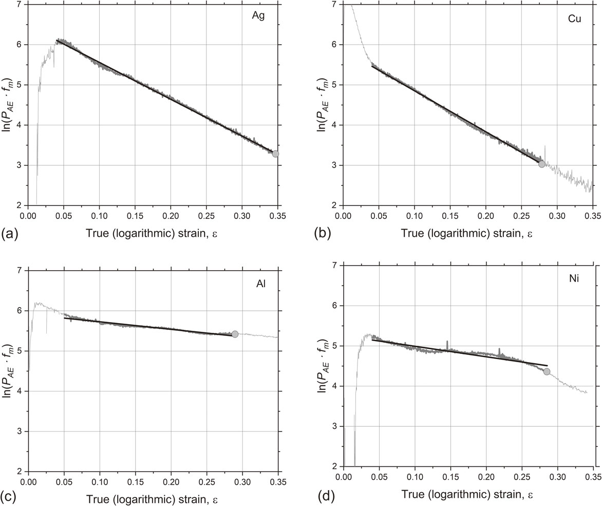
ln(PAE · ( fm − f0)) plotted versus strain, illustrating the linear relation anticipated from eq. (18) for pure fcc metals tested: Ag (a), Cu (b), Al (c), and Ni (d). Straight solid lines represent the result of linear regression. The grey circles indicate the necking points according to the Considère criterion.
From the linear regression analysis applied to the AE data shown in Fig. 6, the k2 values were estimated and compared in Table 1 with those obtained by the non-linear curve fitting of the KM model to the stress-strain data. For all materials tested, the values of k2 evaluated in this way from the AE data appear to be in the reasonable range comparable, albeit at some variance, with those obtained from the KM model. In this section, we discuss the observed results from two aspects: (1) metrology of AE measurements and (2) limitations of the propose modelling approach.
We underline that despite the simplicity of the models used, the k2 values assessed by the AE method appear to be of the correct order of magnitude. The result is remarkable, considering that no calibration of AE measurements has been carried out. Neither we have performed any “tuning” of the AE methodology to optimise its performance for better quantitative agreement with experiments. The AE metrology remains to be an important factor that might affect the result. To reinforce the reliability of the presented findings, it is pertinent to note that the spectral techniques utilised in the ASK algorithm24) used in the present work rely on the well-documented Python Welch spectral routine. In the development of this algorithm, we have tested it extensively against another classic procedure - the Periodogram method described in the earlier works,27,61) where a variety of spectral smoothing windows were probed in application to AE. The Welch method entails segmenting the signal with overlapping sections, applying a window function to each segment, calculating the periodogram for each segment, and subsequently averaging these derived periodograms to yield the estimated PSD.62) Thus, besides the length of the data, the estimation of PSD by the Welch method depends on the segment length, number of fast Fourier transform points NFFT, and percentage of segments overlap. To test the robustness of the estimates reported above, we examined how the variation of these parameters affects the results of calculation of the AE power and median frequency on 10 randomly picked fragments of AE data of 1 s duration for each material. Results are exemplified in Table 2 for Cu. Evidently, although some variability in individual PSD shapes and measured properties was noticed, the results of PAE and fm calculations are stable and not affected by the choice of the Welch parameters varied in the reasonable range, on the average. Similar results are obtained for all materials. The effect of oversampling by acquiring data with a frequency much higher than the Nyquist frequency (up to 10 MHz) was tested in our early experiments on CuZn alloys52) (although not reported in detail). While the computation cost increased dramatically and the artefact frequencies appeared in the spectral density, no benefits for the estimation of the AE power or other spectral properties were noted.
;%0A%09%09%09newWindow.document.open();%0A%09%09%09newWindow.document.write('<img src=%22./Graphics/MT-M2023166tab02.jpg%22>');%0A%09%09%09newWindow.document.close();%0A%09%09)
In addition to computational procedures, we believe that a crucial metrological factor influencing all spectral assessments is the sensor response. Ideally, the transducer should exhibit a higher sensitivity and possess a wider band with a nearly flat response. A higher sensitivity is desired, in particular, to increase the signal-to-noise ratio, which is never very high when AE is caused by dislocation mechanisms. Since the AE signal is buried in the background electric noise, the effect of noise in the estimates of spectral properties has to be taken into account with care (although spectral noise subtraction is implemented in ASK codes, the effectiveness or robustness of this procedure remains uncertain). Testing a relatively high strain rate helps to partly alleviate this issue because the AE level increases with $\dot{\varepsilon }$ as has been discussed above. The strain rate sensitivity of FCC metals, predominantly reflected in Taylor’s a in eq. (6) and, of course, in the dynamic recovery coefficient, is low and can be disregarded in the assessment of the k2 value. This has been noticed in Ref. 52), where several CuZn alloys were tested at two strain rates of 3 × 10⁻² s−1 and 1 × 10⁻² s−1 with qualitatively similar results, albeit with appreciably smaller fluctuations of AE parameters measured at the higher strain rate. Thus, the role of the sensor properties, along with the impact of other external factors on the evaluation of the k2 value from the AE PSD estimates, has yet to be explored.
Finally, it would be reasonable to acknowledge that expecting a perfect quantitative agreement between two simplistic models—the Kocks-Mecking type dislocation evolution model and the proposed AE model would be naive. Both models have inherent limitations, grounded in their reliance on an idealised description of the deformation microstructure characterised by a single internal variable - the total dislocation density. For the sake of simplicity, distinctions are not made between immobile and mobile dislocations (with the latter notably pertinent to AE) or between spatially inhomogeneous dislocation distribution in the cell walls and cell interior, among other factors (such as grain size, SFE, etc.). Hence, our work primarily serves as a proof-of-concept.
Understanding the relationship between dislocation dynamic recovery rate and microstructure is crucial in the context of the strain hardening theory. The kinetic coefficient k2 controlling the dislocation dynamic recovery rate conceals a lot uncertainties standing behind the influence of the microstructure on the mechanical response of a deforming material. Of many intrinsic metallurgical factors, the SFE value and grain size are pivotal for dynamic recovery. Notably, higher SFE is associated with greater dislocation mobility because of enhanced propensity to cross-slip.20) Finer grain sizes generally enhance dynamic recovery drastically. The grain boundaries not only act as barriers for dislocation motion thus promoting the probability of dislocation annihilation in their vicinity, but also serve as sinks for gliding dislocations. As a result, dynamic recovery becomes more prominent as a means to accommodate plastic deformation in ultrafine-grained metals and alloys.34,35,47,48) Concerning the distinctions among the materials tested, a notable perplexity may arise. A pronounced correlation between k2 and SFE may be plausibly expected, cf., for example, a work by Prinz et al.63) However, such a correlation is not evident in materials tested, whether derived from stress-strain data or AE streams. This deviation can likely be attributed to the integral nature of the k2 coefficient in the KM model, which encompasses various dislocation annihilation mechanisms. Consequently, it may depend not only on cross-slip kinetics but also on factors such as grain size and properties of grain boundaries acting as dislocation sinks.
It is important to note that the KM model does not explicitly consider grain size effects, an aspect incorporated in the Mecking-Estrin (ME) model.29) In our study, efforts were made to mitigate grain boundary influences by employing well-annealed samples with coarse grains. However, complete elimination of grain boundary effects in polycrystalline materials is impractical, and the considerable variation in grain size among tested materials is acknowledged as a limitation that could be addressed in future experiments.
While a hybrid framework combining KM and ME models could potentially account for grain size effects, such an integration would forfeit the analytical solutions and compromise the current model’s clarity. In this proof-of-concept, we prioritise maintaining the analytical transparency of our model for ease of comprehension, even at the expense of some accuracy. Consequently, the observed disparity in k2 values between AE data and stress-strain curves may not solely result from metrological considerations in AE measurements but could also be attributed to the oversimplification inherent in the single-variable model approach.
Despite the outlined existing technical challenges and knowledge gaps, the fundamental possibility of assessing the quantitative value of the dislocation recovery rate directly from AE measurements is the most thrilling conclusion that can be drawn from the present study. Taking into account the straightforward relation between k2 and the necking strain εN followed from eq. (16),34,35,47,52) the AE method can be advanced to the state when it predicts the strain localisation condition from the beginning of plastic straining.
As a final remark, it is essential to reiterate that the model presented not only captures all experimentally observed trends but also stems from the synergy of dislocation evolution modelling and AE modelling approaches, establishing itself as the main and most remarkable result.
In the present work, a constitutive AE model was probed against experimental data acquired from the monotonic uniaxial tension of pure Ag, Cu, Al and Ni with significantly different stacking fault energies increasing in the order Ag < Cu < Al < Ni. The AE model based on the established dislocation evolution approach was adapted to enable estimating the rate of dynamic dislocation recovery – the parameter entering virtually any theory of strain hardening, and which, in our opinion, governs the onset of necking instability. The AE behaviour in the pure fcc metals tested in the present work is entirely consistent with the model. A remarkable advantage of the current model is that the dynamic dislocation recovery rate can be obtained directly from AE data without referring to the mechanical stress-strain response. The proposed model is not specific to pure fcc metals and may be flexibly adapted for bcc and hcp metals as well as alloys with dislocation-mediated plasticity. Furthermore, we believe that powered by the AE spectral clustering analysis, the proposed approach can form the basis for further experimental and modelling studies applicable to a wider range of metals and alloys, where deformation twinning accompanies dislocation plasticity.
The suggested analytical model solutions significantly enhance the resilience and predictive capacity of the AE technique. With the aid of these solutions, the in-situ AE method facilitates a precise quantitative assessment of the evolution of the dislocation ensemble under load. Given that this evolution invariably results in the localised strain and eventual failure on a macroscopic scale, we demonstrate that it is fundamentally feasible to predict the initiation of plastic instability by analysing AE data collected at much lower strains than those anticipated by the mechanical Considère criterion for the necking instability.
In terms of future prospects, enhancing the predictive capability of the suggested approach necessitates a more profound comprehension of the experimental variables that impact the recorded values. In pursuit of this goal, it is crucial to prioritise the management of sensor responses and the mitigation of ambient noise. Arguably, it is imperative to create a calibration process for data acquisition or, initially, provide guidelines for selecting the most suitable sensor and optimising the spectral noise reduction algorithm. This is essential to prevent potential distortions and inaccuracies in the acoustic emission spectral density function, which could influence the assessment of properties related to dislocation sources.
AV is grateful to MRC for the partial financial support through internal funding. AV wishes to thank Prof. Kanji Ono for encouragement and motivating inspiration leading to creating this work. IY appreciates partial financial support from the Russian Science Foundation through grant-in-aid 22-29-00143.