Abstract
This study was aimed at examining the effect of the number of grains (representing the total measurement area) on the statistical variation of the area average of the kernel average orientation (KAM), denoted as KAMA, ave, as determined through electron backscatter diffraction (EBSD). Moreover, the number of triple junctions required to obtain statistically valid results was investigated. The results indicated that at least 80–100 grains should be evaluated to reduce the statistical dispersion in plastic-strain evaluation using KAMA, ave. The average triple junction KAM (KAMTJ, ave) values near the random boundary tend to be higher than those near coincident site lattice (CSL) boundaries. There was a correlation between plastic strain and average triple-junction KAM (KAMTJ, ave). This study highlights that KAMTJ is useful parameters for evaluating plastic strain around the triple junctions.
1. Introduction
Electron Backscatter Diffraction (EBSD) is an analytical technique that can be used to determine local crystal orientations at the material surface. In EBSD analysis, the crystal orientation is determined using Kikuchi patterns produced by the diffraction of backscatter electrons. As the EBSD can measure small misorientations caused by plastic deformation, it has been used to establish quantitative strain-evaluation methods [1–8]. The evaluation of plastic strain in EBSD analysis includes parameters such as the kernel average misorientation (KAM), which represents the average misorientation between each measurement point and its neighboring points, and the grain orientation spread (GOS), which indicates the average misorientation of all pairs of measurement points within a grain. Nomura et al. [3] evaluated the plastic strain of austenitic stainless steel after high-temperature tensile test using KAM and GOS and highlighted the correlation between the area average of KAM or GOS and amount of plastic strain introduced during the test. Thus, KAM and GOS are typically considered valuable parameters for the quantitative evaluation of plastic strain. In general, KAM is calculated for each measurement point, while GOS is calculated for each grain. Thus, KAM is suitable for strain evaluation in localized areas, such as grain boundaries and triple junctions.
Grain boundaries and triple junctions in polycrystalline materials may serve as crack initiation sites in various fracture modes (e.g., creep, stress corrosion cracking, and hydrogen embrittlement). Additionally, the occurrence of strain promotes the precipitation of precipitates in certain materials [9–12], with grain boundaries and triple junctions being preferred precipitation sites. In this context, a method enabling quantitative evaluation of the plastic strain around these features could facilitate the understanding of precipitation behaviors in polycrystalline materials. Thus, various researchers have focused on strain evaluation around grain boundaries and triple junctions [13–15].
In addition to EBSD as a promising analytical technique for the evaluation of plastic strain in specific regions, alternative strain-evaluation methods exist, such as digital image correlation (DIC) [16], crystal plasticity analysis based on the finite element method (FEM) [17] and three-dimensional X-ray diffraction microscopy (3D-XRD) based on synchrotron radiation [18]. The DIC method enables in situ measurement of the local strain distribution but is limited to surface measurements. Grains at the material surface are considered to be in the plane stress condition, and the deformation of surface grains is less restrained compared with that of grains within the material. Consequently, surface grains experience higher deformation (plastic strain) than inner grains [19]. In comparison, crystal plasticity analysis based on FEM can evaluate the plastic strain at both the surface and inner grains. However, the prohibitive computational cost limits the number of grains used in the model, which renders it challenging to consider the statistical variability of the results. The 3D-XRD approach can also evaluate the plastic strain of the surface and inner grains. However, its application in practical engineering is hindered by the requirement for synchrotron radiation facilities. In contrast, the EBSD analysis can be easily implemented using a device attached to the scanning electron microscope (SEM). In recent years, the performance of the computers and CCD cameras used in EBSD measurement systems has been improved and this enabled the rapid measurement of large areas of specimens.
As the EBSD analysis evaluates small misorientations between the measurement points, precise measurement is crucial to minimize measurement errors. Consequently, efforts are being made to standardize EBSD measurements (ISO TC 202). In Japan, a technical standard for EBSD measurements [20] has already been published by the Society of Materials Science. Notably, in most polycrystalline materials, the grain size exhibits significant dispersion, and the plastic strain distribution may not be uniform. Thus, the number of grains used in EBSD analysis can affect the experimental outcomes. An empirically defined guideline in the technical standards published in Japan [20] suggests that at least 100 grains should be evaluated in EBSD analyses. However, detailed research on the number of grains that should be evaluated to obtain valid results is lacking. Furthermore, although EBSD can evaluate the plastic strain at local areas such as triple junctions, no empirical guidelines exist regarding the number of triple junctions required to evaluate the plastic strain in EBSD analyses.
To address these limitations, this study was aimed at examining the influence of the number of grains on the statistical variation of the area-average KAM. Moreover, the number of triple junctions required to obtain statistically valid results for plastic-strain evaluation around triple junctions was investigated.
2. Experimental Procedure
2.1 Specimens
SUS316NG (nuclear grade) alloy, commonly used in nuclear power plants, was used in the experiments. In particular, the low carbon content of this alloy helps prevent stress corrosion cracking caused by sensitization, and its high nitrogen content helps achieve high strength. Table 1 outlines the chemical composition of the specimen. The specimen microstructure consisted of equiaxed grains. Precipitates, such as carbide and nitride, were not observed in the specimen. The average grain size was approximately 180 µm when the twin boundaries in the grains were ignored in the grain-size calculation and approximately 100 µm when the twin boundaries were considered as grain boundaries. The grain size was calculated as mean area diameter. The mean area diameter (Dmean) was calculated by eq. (1):
| \begin{equation}
D_{\textit{mean}} = \frac{\displaystyle\sum\nolimits_{i = 1}^{n} (A_{i} \cdot D_{i})}{\displaystyle\sum\nolimits_{i = 1}^{n} A_{i}}
\end{equation}
| (1) |
where Ai is the area of the ith grain, and Di is the diameter of the ith grain. n is the total number of the grains. Di was calculated as the equivalent circle diameter in this study.
Table 1 Chemical composition of specimen used in this study (mass%).

Tensile specimens with a gauge length of 30 mm and diameter of 6 mm were prepared. Uniaxial tensile tests were conducted at a strain rate of 1.67 × 10⁻³ s−1 and room temperature. The tensile tests were interrupted before rupture to obtain 5%, 10%, and 15% deformed specimens.
2.3 EBSD analysis
Following the interrupted tensile tests, the tensile specimens were cut in the longitudinal direction at the gauge portion and embedded in conductive resin. The cross-section of the cut specimen was polished using waterproof abrasive papers, a diamond slurry, and a colloidal silica suspension. Orientation imaging microscopy (OIM, TSL Solutions Inc.) was used for the EBSD measurement. The accelerating voltage was 20 kV, and the working distance was 15 mm. Measurements were obtained at the center of the gauge portion, with each measurement area sized 400 × 1000 µm and 10 areas measured for each specimen. The scanning pitch was 2 µm. The average confidence index, representing the indexing accuracy of the Kikuchi patterns, was 0.8, and the average fit value was approximately 0.6° for all measurement data. Thus, the data quality was considered to be adequately high. Each measurement area contained approximately 30 grains when the twin boundaries in the grains were not recognized as grain boundaries. Otherwise, the number of grains in a single measurement area was approximately 150. The OIM Analysis (ver. 8.0, TSL Solutions Inc.) software was used to examine the measurement data.
For the evaluation of plastic strain around the triple junctions, KAMTJ was used. The definition of KAMTJ is shown in Fig. 1. KAMTJ was calculated at every triple junction in the measured area as follows:
-
1.
Select the nearest measurement point to the triple junction, which is used as a reference point in the next step (Fig. 1(a)).
-
2.
Extract all measurement points within 3 pixels from the reference point (Fig. 1(b)). These measurement points belong to the same grain.
-
3.
Obtain KAM values from all extracted points.
-
4.
Select five measurement points which have the highest KAM value among all extracted points (Fig. 1(c)).
-
5.
Calculate KAMTJ using eq. (2):
| \begin{equation}
\mathit{KAM}_{\text{TJ}} = \frac{\displaystyle\sum\nolimits_{i = 1}^{5} \mathit{KAM}_{\text{TJ},i}}{5}
\end{equation}
| (2) |
where
KAMTJ, i is the KAM value of the
ith selected point. Because a triple junction is composed of three grains, three different
KAMTJ values are determined from one triple junction. Moreover, a triple junction is expressed as an intersection of three grain boundaries in the EBSD analysis. Grain boundaries can be classified into two types: grain boundaries with a coincidence site lattice (CSL) [
21–
23], termed CSL boundaries, and high-angle grain boundaries without CSLs, termed random boundaries. Based on the combinations of CSL and random boundaries, four types of triple junctions can be identified, as shown in
Fig. 2. In most previous studies on strain evaluation near triple junctions [
24–
27], the four types of triple junctions were distinguished. Thus, in this study, these four types of triple junctions were distinguished in the strain evaluation using
KAMTJ.
Brandon’s criteria [21] were used as tolerance angle in the judgement of CSL boundaries. In the Brandon’s criteria, the tolerance angle Δθ can be calculated using eq. (3):
| \begin{equation}
\Delta \theta = \frac{K}{\Sigma^{n}}
\end{equation}
| (3) |
where K and n are constants. In this study, K = 15° and n = 0.5 were used for the calculation. Thus, Δθ for Σ3 (Σ = 3) boundary was calculated as 8.66°. Because nearly all the CSL boundaries observed in the specimens were Σ3, only these boundaries were considered CSL boundaries in the subsequent discussions. In EBSD analyses, twin boundaries observed in face-centered cubic metals are recognized as Σ3 boundaries, rendering it challenging to differentiate twin boundaries and Σ3 boundaries. Therefore, these boundaries were not distinguished in this study.
KAMTJ could not be automatically calculated using OIM Analysis. Therefore, an in-house program was prepared using Python ver. 3.9.12 to compute KAMTJ, and the calculation process is shown in Fig. 3.
3. Results and Discussion
3.1 Strain evaluation by area average of KAM
Figure 4 shows inverse pole figure (IPF) maps of the as-received and deformed specimens, with black lines representing grain boundaries with a misorientation angle larger than 5°. KAM maps of the as-received and the deformed specimens are shown in Fig. 5. As the plastic strain of the specimen increased, the number of measurement points with higher KAM values increased. These points distributed mostly around the grain boundaries.
The distribution of the KAM value is shown in Fig. 6. The lower horizontal axis represents the logarithm of KAM values. The distribution of log(KAM) seems to follow the log-normal distribution. Kamaya et al. [28] reported that the distribution of the local misorientation which is a similar parameter to KAM can be represented by the log-normal distribution. Thus, the results obtained in this study seems to be in a good agreement with Kamaya’s report. The average KAM in the measured area, KAMA, ave was calculated using eq. (4):
| \begin{equation}
\mathit{KAM}_{\text{A,$\,$ave}} = 10^{\left(\frac{\sum_{i = 1}^{n} \log(\mathit{KAM}_{i})}{n}\right)}
\end{equation}
| (4) |
where KAMi is the KAM value of the ith measurement point and n is the total number of measurement points in the measured area. Since the distribution of the KAM value follows the log-normal distribution, KAMA, ave was calculated as the geometric mean value. Figure 7 shows the relationship between the plastic strain and KAMA, ave. Consistent with previously reported results [3], a strong correlation was observed between the plastic strain and KAMA, ave.
According to the law of large numbers, KAMA, ave tends to approach the population mean when the number of grains used for its calculation increases. Therefore, the relationship between the number of grains used for calculating KAMA, ave and the 99% confidence intervals for the population mean of KAMA, ave was investigated. To this end, a new parameter, KAMG, ave, was defined as in eq. (5):
| \begin{equation}
\mathit{KAM}_{\text{G,$\,$ave}} = 10^{\left(\frac{\sum_{i = 1}^{m} \log(\mathit{KAM}_{\text{in grain},\,i})}{m}\right)}
\end{equation}
| (5) |
where m is the number of measurement points in a specific grain, and KAMin grain, i is the KAM value at the ith measurement point in the grain. In this study, a single measurement area contained approximately 150 grains when the twin boundaries were considered grain boundaries. Thus, the average of KAMG, ave obtained from 150 grains could be approximated to KAMA, ave, as indicated in eq. (6):
| \begin{equation}
\mathit{KAM}_{\text{A,$\,$ave}} \cong \frac{\displaystyle\sum\nolimits_{j = 1}^{N} \mathit{KAM}_{\text{G,$\,$ave},\,j}}{N}
\end{equation}
| (6) |
where N is the number of the grains in one measurement area (around 150, in this study), and KAMG, ave, j is the KAMG, ave value of the jth grain. KAMG, ave was calculated for the tensile specimens with 0–15% plastic strain. For each specimen, approximately 1400 grains were used when the twin boundaries were considered grain boundaries. Additionally, the average and standard deviation of KAMG, ave were determined and used to specify the 99% confidence intervals for the population mean of KAMG, ave. To clarify the influence of the number of grains on the 99% confidence interval width, the 99% confidence intervals were expressed as a function of the number of grains used to compute the average KAMG, ave. The results are shown in Fig. 8. There are two types of curves in the figure, one is 99% upper limit which decreases with increasing the number of grains. The other is 99% lower limit which increases with increasing the number of grains. The 99% confidence interval width decreased as the number of grains increased, across all plastic strain levels. The interval width stabilized after the number of grains exceeded 400–500. This outcome indicated that in EBSD analyses, the number of grains used for strain evaluation by KAMA, ave should be more than 400–500 when the twin boundaries are considered as grain boundaries. When the twin boundaries in the grains are ignored, approximately 80–100 grains should be used.

Kamaya et al. [8] investigated misorientation identification errors in EBSD measurements, focusing on the change in KAM values with variations in the distance of neighboring points used for KAM calculation. The authors highlighted a linear relationship between the distance of neighboring points and KAM values and noted that the intercept of the regression line represents the amount of error in the misorientation identification. Therefore, in this study, Kamaya’s method was used to examine the misorientation identification error in EBSD measurements, yielding values of 0.24°, 0.24°, 0.36°, and 0.53° for the specimens subjected to 0% (as-received), 5%, 10%, and 15% strain levels. As shown in Fig. 8, the 99% confidence interval widths were smaller than Kamaya’s parameter when the number of grains were 400–500, suggesting that the statistical variation in KAMG, ave attributable to the number of evaluated grains is less significant than the misorientation identification error.
3.2 Evaluation of plastic strain around grain boundaries and triple junctions
The plastic strain around grain boundaries was evaluated using KAMGB, ave. KAMGB, ave was defined as the average KAM calculated from the measurement points within an arbitrary distance from the grain boundaries, as indicated in eq. (7) and illustrated schematically in Fig. 9:
| \begin{equation}
\mathit{KAM}_{\text{GB,$\,$ave}} = 10^{\left(\frac{\sum_{i = 1}^{n_{\text{GB}}} \log (\mathit{KAM}_{\text{GB},\,i})}{n_{\text{GB}}}\right)}
\end{equation}
| (7) |
where KAMGB, i is the KAM value of the ith measurement point near the grain boundary, and nGB is the total number of points extracted near grain boundaries. Since the distribution of KAM value follows the log-normal distribution, KAMGB, ave was also calculated as geometric mean value. Notably, nGB varies with the maximum distance from the grain boundary used for calculating KAMGB, ave, as shown in Figs. 9(a)–(d). Moreover, the distance from the grain boundary takes discrete value owing to the principle of EBSD measurements. Thus, the distance from the grain boundary is expressed as a multiple of the scanning pitch in EBSD measurements (in this study, 2, 4, 6 µm…). Figure 10 shows the relationship between the number of pixels extracted from grain boundary and KAMGB, ave, normalized by KAMA, ave. For each specimen, the KAMGB, ave/KAMA, ave values were larger than 1.0 and decreased with increasing number of the pixels. Thus, KAM values were higher at the grain boundaries than those for the inner grains.


KAM values around the triple junctions were evaluated using KAMTJ. As shown in Fig. 2, triple junctions can be classified into four types based on the combination of random or CSL boundaries. Figure 11 shows the proportion of the R-R-R, R-R-C and R-C-C type triple junctions of the specimens. The proportion of R-R-R type triple junctions increased with increasing the plastic strain. On the other hand, the proportions of R-R-C and R-C-C type triple junctions decreased with increasing the plastic strain. In this study, tolerance angle of 8.66° was used for the judgement of Σ3 type CSL boundary. When the plastic strain increases, the misorientation around the grain boundary increases. Therefore, it is considered that the deviation from ideal CSL relationship can also increase at the CSL boundary after the plastic deformation. If the deviation exceeds the tolerance angle of 8.66°, the CSL boundary is not judged as CSL boundary, and recognized as random boundary in the EBSD analysis software. This can be the reason for the change in the proportion of R-R-R, R-R-C and R-C-C type triple junctions after the plastic deformation.
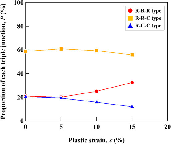
Figure 12 shows the distribution of KAMTJ. The types of triple junctions were not distinguished in Fig. 12. The distribution of log(KAMTJ) seems to follow the normal distribution. Therefore, it is considered that distribution of KAMTJ follows the log-normal distribution. The average of KAMTJ (KAMTJ, ave) was calculated as geometric mean value using eq. (8):
| \begin{equation}
\mathit{KAM}_{\text{TJ,$\,$ave}} = 10^{\left(\frac{\sum_{i = 1}^{n_{\text{TJ}}} \log (\mathit{KAM}_{\text{TJ},i})}{n_{\text{TJ}}}\right)}
\end{equation}
| (8) |
where KAMTJ, i is the KAMTJ value of the ith measurement point, and nTJ is the total number of the triple junctions. KAMTJ, ave was calculated for each type of triple junctions. Figure 13 shows the relationship between the plastic strain and KAMTJ, ave. There was a strong correlation between the plastic strain and KAMTJ, ave. KAMTJ, ave increased linearly with increasing the plastic strain when the plastic strain was 0–10%. On the other hand, KAMTJ, ave at 15% plastic strain was slightly lower than that of expected from the linear relationship. When comparing the KAMTJ, ave at each type of triple junctions, KAMTJ, ave at R-R-R type triple junctions was slightly higher than that at the others, especially at 10% and 15% deformed specimens. In the specimens with 0–15% deformation, KAMTJ, ave on the R-R side of the R-R-C type triple junction was approximately 6.6–9.6% higher than that on the R-C side. Moreover, KAMTJ on the R-C side of the R-C-C type triple junction was approximately 3.5–8.4% higher than that on the C-C side. It is reported that the strain tends to be higher on the R-R side of R-R-C type triple junction compared with R-C side [27]. The same result was obtained in our study. The reason for this result is not fully clarified and further investigation is required. However, the difference in KAMTJ, ave for each type of triple junctions was not significant and the relationship between the plastic strain and there was a strong correlation between the plastic strain and KAMTJ, ave. Thus, this relationship can be used for the plastic strain evaluation of deformed materials.

Since it is considered that KAMTJ, ave can be used for the plastic strain evaluation, a statistically appropriate number of the triple junctions which should be used for the strain evaluation using KAMTJ, ave was investigated. Figure 14 shows the relationship between the number of the triple junctions used for the evaluation and the 99% confidence interval of KAMTJ, ave. The types of triple junction were not distinguished in Fig. 14. The 99% confidence interval decreased with increasing the number of triple junctions used for the evaluation. The interval width stabilized after the number of grains exceeded 200. Thus, it is recommended that at least 200 triple junctions should be evaluated for accurate strain evaluation using KAMTJ, ave.
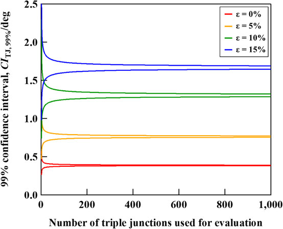
As mentioned above, evaluation of the plastic strain using KAMA, ave requires around 80–100 grains to obtain the accurate result. When we compare the Fig. 8 and Fig. 14, the 99% confidence intervals of KAMA, ave is larger than that of KAMTJ, ave, especially at the higher strain. Additionally, the number of triple junctions is larger than the number of grains in the EBSD measurement area in most cases. In this study, the number of the triple junctions were three to four times larger than the number of the grain. These results implies that KAMTJ, ave is a good parameter for the evaluation of the plastic strain because it may require smaller measurement areas compared with KAMA, ave.
4. Conclusion
The influence of the number of grains on the results of strain evaluation using KAMA, ave was investigated. Moreover, the number of triple junctions required to obtain statistically valid results was assessed. The following key conclusions were derived:
-
(1)
To minimize statistical dispersion in plastic-strain evaluation using KAMA, ave, at least 80–100 grains should be evaluated, when the twin boundaries within the grain were ignored.
-
(2)
To obtain statistically appropriate results in strain assessment using KAMTJ, at least 200 triple junctions should be evaluated for each specimen.
-
(3)
KAMTJ, ave tends to be higher on the R-R side of the R-R-C type triple junction compared with that on the R-C side. In addition, KAMTJ, ave on the R-C side of the R-C-C type triple junction is higher than that on the C-C side.
-
(4)
KAMTJ, ave can serve as valuable tools for the evaluation of plastic strain of damaged materials. Moreover, this parameter can be used in other investigations, such as understanding fracture mechanisms or the effect of strain on the precipitation behaviors of precipitates at triple junctions.
REFERENCES
- 1) Y. Sakakibara, K. Kubushiro and G. Nakayama: Distribution of Misorientation at Grain Boundary by EBSD for Low Carbon Stainless Steel Strained by Various Deformation Modes, J. Japan Inst. Metals 74 (2010) 258–263. doi:10.2320/jinstmet.74.258
- 2) Y. Sakakibara, K. Nomura, K. Kubushiro and H. Yoshizawa: Plastic Strain Dependency of Misorientation for Austenitic Stainless Steel and Nickel Base Alloy, J. Japan Inst. Metals 76 (2012) 669–676. doi:10.2320/jinstmet.76.669
- 3) K. Nomura, K. Kubushiro, Y. Sakakibara, S. Takahashi and H. Yoshizawa: Effect of Grain Size on Plastic Strain Analysis by EBSD for Austenitic Stainless Steels with Tensile Strain at 650°C, J. Soc. Mater. Sci. Jpn. 61 (2012) 371–376. doi:10.2472/jsms.61.371
- 4) K. Nomura, Y. Shioda, K. Kubushiro, H. Nakagawa and Y. Murata: Strain Analysis of Weld Joint of 23Cr-45Ni-7W Alloy by XRD and EBSD Method, J. Soc. Mater. Sci. Jpn. 66 (2017) 51–57. doi:10.2472/jsms.66.51
- 5) K. Kubushiro, Y. Sakakibara and T. Ohtani: Creep Strain Analysis of Austenitic Stainless Steel by SEM/EBSD, J. Soc. Mater. Sci. Jpn. 64 (2015) 106–112. doi:10.2472/jsms.64.106
- 6) H. Hirai, K. Kubushiro and S. Yusa: Proceedings of the 60th JSMS Annual Meetings, 60, (2011) pp. 256–266.
- 7) M. Kamaya: Measurement of Plastic Strain Distribution by Electron Backscatter Diffraction, J. Soc. Mater. Sci. Jpn. 58 (2009) 568–574. doi:10.2472/jsms.58.568
- 8) M. Kamaya, Y. Sakakibara, R. Yoda, S. Suzuki, H. Morita, D. Kobayashi, K. Yamagiwa, T. Nishioka, Y. Maekawa, T. Tanakamaru, H. Nagashima and T. Ohtani: A round robin EBSD measurement for quantitative assessment of small plastic strain, Mater. Charact. 170 (2020) 110662. doi:10.1016/j.matchar.2020.110662
- 9) K. Kawasaki and M. Matsuo: Deformation Structures as Nucleation Sites for Recrystallization, Tetsu-to-Hagané 70 (1984) 1808–1815. doi:10.2355/tetsutohagane1955.70.15_1808
- 10) J.M. Vitek and S.A. David: The Sigma Phase Transformation in Austenitic Stainless Steels, Weld. J. 65 (1986) 106–111.
- 11) T. Hirata and S. Matsuo: The Effect of Plastic Deformation on the Precipitation in an Al-Mg-Si Alloy, J. Japan Inst. Metals 36 (1972) 1159–1163. doi:10.2320/jinstmet1952.36.12_1159
- 12) S. Yamamoto, Y. Yamamoto and Y. Murakami: Effects of Plastic Deformation on the Age-hardening of Cu-Be Alloys, J. Japan Inst. Metals 37 (1973) 1268–1275. doi:10.2320/jinstmet1952.37.12_1268
- 13) C. Ma, J. Mei, Q. Peng, P. Deng, E.H. Han and W. Ke: Microstructure Characterization of the Fusion Zone of an Alloy 600-82 Weld Joint, J. Mater. Sci. Technol. 31 (2015) 1011–1017. doi:10.1016/j.jmst.2015.08.013
- 14) C.S. Yun, K.T. Lui and J.C. Kuo: Orientation Characterization of Columnar-Grained Aluminum at Triple Junctions, Mater. Trans. 50 (2009) 2493–2497. doi:10.2320/matertrans.M2009159
- 15) R.K. Davies and V. Randle: Orientation perturbations near triple junctions in a non-cell forming aluminium–magnesium alloy, Mater. Sci. Eng. A 283 (2000) 251–265. doi:10.1016/S0921-5093(00)00618-3
- 16) N. Koga: Visualization of Strain Distribution in Metal Materials by Digital Image Correlation Method, Mater. Jpn. 55 (2016) 267–270. doi:10.2320/materia.55.267
- 17) M.A. Charpagne, J.M. Hestroffer, A.T. Polonsky, M.P. Echlin, D. Texier, V. Valle, I.J. Beyerlein, T.M. Pollock and J.C. Stinville: Slip localization in Inconel 718: A three-dimensional and statistical perspective, Acta Mater. 215 (2021) 117037. doi:10.1016/j.actamat.2021.117037
- 18) Y. Hayashi, Y. Hirose, D. Setoyama and Y. Seno: Orientation and stress mapping in polycrystalline materials by the scanning 3DXRD method, J. Jpn. Soc. Synchrotron Radiat. Res. 31 (2018) 257–265.
- 19) H. Kimura, Y. Wang, Y. Akiniwa and K. Tanaka: Misorientation Analysis of Plastic Deformation of Austenitic Stainless Steel by EBSD and X-Ray Diffraction Methods, Trans. Jpn. Soc. Mech. Eng. A 71 (2005) 1722–1728. doi:10.1299/kikaia.71.1722
- 20) JSMS Committee on High Temperature Strength of Materials: Standard for misorientation analysis by electron backscatter diffraction (EBSD) for material characterization, JSMS-SD-15-01, (2016).
- 21) D.G. Brandon, B. Ralph, S. Ranganathan and M.S. Wald: A field ion microscope study of atomic configuration at grain boundaries, Acta Metall. 12 (1964) 813–821. doi:10.1016/0001-6160(64)90175-0
- 22) H. Kokawa: Grain Boundary Engineering —Application to Austenitic Stainless Steels (I) ∼Character and Behavior of Grain Boundaries∼, Mater. Jpn. 52 (2013) 10–13. doi:10.2320/materia.52.10
- 23) Y. Ishida: Kinzoku Kessho Ryukai no Kouzou, Nihon Kessho Gakkaishi 12 (1970) 142–153. doi:10.5940/jcrsj.12.142
- 24) P. Fortier, W.A. Miller and K.T. Aust: Triple junction and grain boundary character distributions in metallic materials, Acta Mater. 45 (1997) 3459–3467. doi:10.1016/S1359-6454(97)00004-9
- 25) L. Tanure, D. Terentyev, V. Nikolić, J. Riesch and K. Verbeken: EBSD characterization of pure and K-doped tungsten fibers annealed at different temperatures, J. Nucl. Mater. 537 (2020) 152201. doi:10.1016/j.jnucmat.2020.152201
- 26) X. Zhang, S. Guo and J. Zhong: Microevolution of grain boundary character distribution in Hastelloy C-276 during the annealing process, J. Mater. Res. Technol. 18 (2022) 1534–1541. doi:10.1016/j.jmrt.2022.03.056
- 27) S. Kobayashi, T. Inomata, H. Kobayashi, S. Tsurekawa and T. Watanabe: Effects of grain boundary- and triple junction-character on intergranular fatigue crack nucleation in polycrystalline aluminum, J. Mater. Sci. 43 (2008) 3792–3799. doi:10.1007/s10853-007-2236-z
- 28) M. Kamaya: Characterization of microstructural damage due to low-cycle fatigue by EBSD observation, Mater. Charact. 60 (2009) 1454–1462. doi:10.1016/j.matchar.2009.07.003
Nomenclature list
KAMAverage misorientation between neighboring points
KAMA, aveKAM value averaged in the measurement area
KAMGB, aveAverage KAM calculated using measurement points near the grain boundary
KAMTJAverage KAM calculated using measurement points near the triple junction
KAMGB, aveAverage KAM calculated using all measurement points in a single grain
GOSAverage misorientation of all pairs of measurement points within a grain

;%0A%09%09%09newWindow.document.open();%0A%09%09%09newWindow.document.write('<img src=%22./Graphics/MT-Z2023013tab01.jpg%22>');%0A%09%09%09newWindow.document.close();%0A%09%09)


