Geometrical Conversion of the EGFR Extracellular Domain by Adiabatic Mapping Combining Normal Mode Analysis of the Elastic Network Model and Energy Optimization

Abstract

The activation of epidermal growth factor receptor (EGFR) involves the geometrical conversion of the extracellular domain (ECD) from the tethered to the extended forms with the dynamic rearrangement of the relative positions of four subdomains (SDs); however, this conversion process has not yet been thoroughly understood. We compare the two different forms of the X-ray crystal structures of ECD and simulate the ECD conversion process using adiabatic mapping that combines normal mode analysis of the elastic network model (ENM-NMA) and energy optimization. A comparison of the crystal structures reveals the rigidity of the intradomain geometry of the SD-I and -III backbone regardless of the form. The forward mapping from the tethered to the extended forms retains the intradomain geometry of the SD-I and -III backbone and reveals the trends to rearrange the relative positions of SD-I and -III and to dissociate the C-terminal tail of SD-IV from the hairpin loop in SD-II. The reverse mapping from the extended to the tethered forms complements the promotion of ECD conversion in the presence of epidermal growth factor (EGF).

Introduction

Epidermal growth factor receptor (EGFR) is a member of the ErbB family of receptor tyrosine kinases, which regulate cell growth, differentiation, migration and proliferation. Current cancer therapeutic strategies target EGFR because colon, rectum and lung cancer cells overexpress EGFR relative to adjacent normal cells. EGFR comprises an extracellular domain (ECD), a transmembrane peptide, an intracellular juxtamembrane segment, a tyrosine kinase domain (TKD) and a C-terminal regulatory tail. The EGFR signal transduction system is activated by binding of epidermal growth factor (EGF)^1,2) or transforming growth factor-α (TGF-α)³⁾ to an ECD, dimerization of two ECDs and tyrosine phosphorylation of TKD. Gefitinib,⁴⁾ erlotinib,⁵⁾ afatinib⁶⁾ and osimertinib,⁷⁾ which are used in the treatment of lung cancer, are TKD inhibitors, whereas cetuximab^8,9) and panitumumab,¹⁰⁾ which are used in the treatment of colon and rectal cancers, are anti-EGFR antibodies to inhibit ligand binding to ECD.

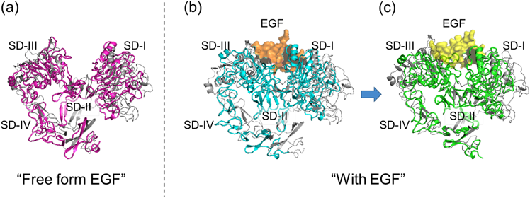
The X-ray crystal structures of ECDs that have currently been identified reveal that ECD adopts two forms in which the relative positions of four subdomains (SDs) are different: First is the monomer structure co-crystalized with EGF, antibody or other proteins, where the hairpin loop in SD-II and the C-terminal tail of SD-IV are intramolecularly tethered (so-called the tethered form, Fig. 1a).^8,9,11–14) The other is the EGF : ECD = 2 : 2 complex structure, where the above tether is completely dissociated (so-called the extended form, Fig. 1b).^1,3,15) EGFR activation involves the dynamic geometrical ECD conversion from the tethered to the extended forms.

Fig. 1. Tethered Form (a, PDB ID 1NQL) and Dimerized Extended Form (b, PDB ID 3NJP)

SD-I, -II, -III and -IV are colored yellow, cyan, magenta and green, respectively. The two EGFs are colored brown in (b). (Color figure can be accessed in the online version.)

The process of ECD conversion is not yet thoroughly understood. Computer simulation is very useful to depict micro phenomena on a molecular level because such phenomena are impossible to observe directly. Molecular dynamics (MD) simulation is the most powerful and represented tool for such simulations, and some MD simulations have been performed for the observation of ECD.^16–19) These simulations have derived useful knowledge but were insufficient because the time cost had to be limited to monitor the entire ECD conversion. Here, we have simulated the ECD conversion between the two forms by adiabatic mapping that combines normal mode analysis (NMA) and energy optimization using a molecular force field. NMA has the advantage of being free from time costs compared with MD simulation, but the conventional NMA using only the force-field parameter needs a “strict” energy-optimized structure so as not to fall into the negative eigenvalue problem.^20–23) The optimization sometimes involves a large time cost and the optimized structure often deviates from its original structure. To resolve this issue, we adopt NMA using the elastic network model (ENM-NMA), where the potential functions are solely harmonic terms with equilibrium positions residing on the studied structure.^24–36) This method does not require energy optimization and is appropriate to describe only low frequency normal modes that express collective motion such as interdomain motion. In this study, we comprehensively compare the X-ray crystal structures of ECD taken from The Protein Data Bank (PDB),³⁷⁾ and discuss the process of ECD conversion by adiabatic mapping between the tethered and the extended forms.

Results

Geometrical Comparison of X-Ray Crystal Structures

The PDB profiles of the tethered and the extended forms for the comparison of X-ray crystal structures are listed in Table 1. The geometrical similarity was compared among the seven tethered forms, among the six extended forms, and between the tethered and the extended forms. The root-mean-square deviation (RMSD) was calculated for each SD, and for SD-I and -III (Table 2).

Table 1. Profile of X-Ray Crystal Structures of ECD Used in This Study

Form	PDBa)	Resolution/Å	Missing residueb)	Sequential difference (vs. 1NQL)	Ligand	Distance between SD-I and -IIIc)/Å
Tethered	1NQL	2.8	1–2	—	EGF	55.4
	1YY9	2.61	1	S474K, E610R	Cetuximab (antibody)	63.7
	3QWQ	2.75	1	K516N	Adnectin (monobody)	56.5
	4KRO	3.05	1–3, 101–107, 184–207, 605–614	K516N	Cetuximab/Nanobody/VHH domain EGA1	59.5
	4KRP	2.82	1–3, 133–207, 613–614	K516N	Cetuximab/Nanobody/VHH domain 9G8	59.2
	4UIP	2.95	1, 614	K516N	Repebody (rAC1)	61.3
	4UV7	2.1	147–163, 614	K516N	GC1118A (antibody)	56.3
Extended	3NJP_A	3.3	—	—	EGF	38.2
	3NJP_B		—	—	EGF	38.1
	1IVO_A	3.3	1, 513–614	—	EGF	38.2
	1IVO_B		1–2, 513–614	—	EGF	38.0
	1MOX_A	2.5	306, 501–614	—	TGF-α	37.8
	1MOX_B		502–614	—	TGF-α	37.7

a) PDBs of boldface type were adopted as basic initial structures for adiabatic mapping. b) Residue missing all atoms was listed from residues consisting of ECD (residue 1–614). c) The distance was calculated from the geometrical center of each subdomain (SD-I; residue 4–186, SD-III; residue 310–481). The geometrical center was determined using only Cα atoms.

Table 2. Root-Mean-Square Deviation (RMSD (Å)) between X-Ray Crystal Structures

SD-Xa)		SD-I	SD-II	SD-III	SD-IV	SD-I and -III
Among tethered forms	Average	0.67	1.58	0.63	0.91	3.28
	Min	0.40	0.90	0.27	0.56	0.47
	Max	0.94	3.00	1.10	1.36	7.43
Among extended forms	Average	0.73	1.04	0.59	—	1.04
	Min	0.31	0.49	0.35	—	0.51
	Max	1.00	1.49	0.82	—	1.65
Between tethered and extended forms	Average	0.76	2.73	0.80	0.97	17.9
	Min	0.53	2.27	0.56	0.72	16.6
	Max	0.97	3.20	1.30	1.26	18.7

a) The RMSD for SD-X (X = I, II, III, IV or “I and -III”) was calculated after fitting for only corresponding SD-X.

For the comparison among the seven tethered forms, the average RMSDs for SD-I and for SD-III were 0.67 Å and 0.63 Å, respectively. These values meant that the intradomain geometry of the SD-I and -III backbone was similar among the seven tethered forms. The average RMSD for SD-I and -III was 3.28 Å, which indicated that the relative positions of SD-I and -III deviated. The maximal RMSD for SD-I and -III was 7.43 Å between 1NQL and 1YY9. The difference was reflected in the angle deviation of the relative positions of SD-I and -III (32.9°, Fig. 2 and Table 3). The other tethered forms took an intermediate relative position of SD-I and -III between those of 1NQL¹¹⁾ and 1YY9⁸⁾ (Fig. 2 and Table 3).

Fig. 2. Superposition of X-Ray Crystal Structures among Three Tethered Forms (1NQL: Green; 1YY9: Cyan; 4UIP: Magenta) Fitted with Respect to SD-I

Yellow sphere (X) shows the geometrical center of SD-I, and green (Y), cyan (Z) and magenta (W) spheres show the geometrical center of SD-III of each PDB. The three structures are superimposed after fitting for SD-I. (Color figure can be accessed in the online version.)

Table 3. Angle (degrees) of SD1-III Central Axis between 2 PDBs after Fitting for SD-I

Form		Tethered							Extended
	PDB	1NQL	1YY9	3QWQ	4KRO	4KRP	4UIP	4UV7	1IVO _A	1IVO _B	1MOX _A	1MOX _B	3NJP _A	3NJP _B
Tethered	1NQL	—	—	—	—	—	—	—	—	—	—	—	—	—
	1YY9	32.9	—	—	—	—	—	—	—	—	—	—	—	—
	3QWQ	6.8	27.6	—	—	—	—	—	—	—	—	—	—	—
	4KRO	14.0	19.3	8.4	—	—	—	—	—	—	—	—	—	—
	4KRP	16.2	17.1	10.4	2.1	—	—	—	—	—	—	—	—	—
	4UIP	14.5	18.8	8.8	0.7	2.1	—	—	—	—	—	—	—	—
	4UV7	4.1	30.4	2.9	11.3	13.2	11.7		—	—	—	—	—	—
Extended	1IVO_A	33.5	1.6	28.3	20.0	17.9	19.6	31.0	—	—	—	—	—	—
	1IVO_B	33.9	2.2	28.8	20.5	18.2	20.1	31.6	0.7	—	—	—	—	—
	1MOX_A	30.7	3.4	25.8	17.5	15.3	17.1	28.2	3.0	3.2	—	—	—	—
	1MOX_B	32.5	0.9	27.3	19.0	16.5	18.5	29.7	1.2	1.9	2.5	—	—	—
	3NJP_A	33.6	1.4	28.5	20.1	18.1	19.7	31.2	0.3	0.8	3.2	1.2	—	—
	3NJP_B	34.1	2.0	29.0	20.6	18.4	20.3	31.6	0.7	0.4	3.5	1.8	0.6	—

For the comparison among the six extended forms, the average RMSDs for SD-I and for SD-III were 0.73 Å and 0.59 Å, respectively. These values meant that the intradomain geometry of the SD-I and -III backbone was similar among the six extended forms. The average RMSD for SD-I and -III was 1.04 Å, which indicated that the deviation of the relative positions of SD-I and -III was smaller among the six extended forms than among the seven tethered forms.

For the comparison between the tethered and extended forms, the average RMSDs for SD-I and for SD-III were 0.76 and 0.80 Å, respectively. These values meant that the intradomain geometry of the SD-I and -III backbone was similar between the tethered and extended forms. The average RMSD for SD-I and -III was 17.9 Å, which indicated that the relative positions of SD-I and -III were quite different between the tethered and the extended forms.

Adiabatic Mapping among the Tethered Forms

1NQL, 1YY9 and 4UIP¹³⁾ (without proteins other than the ECD) were selected for the mapping because the relative positions of SD-I and -III in 1NQL and 1YY9 were very different, and because 4UIP took an intermediate position between the other two (Fig. 2).

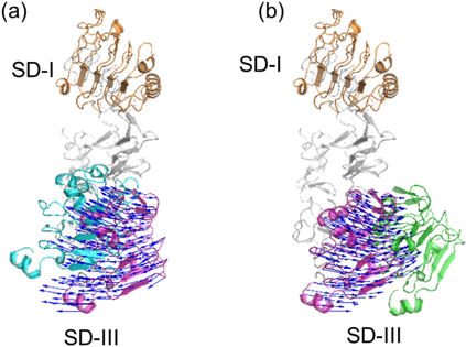
The mapping between 1NQL and 4UIP smoothly decreased RMSD for all SDs until the 4th cycle and reached the minimal RMSDs at the 8th cycle (Fig. 3a, the leftmost frame). The minimal RMSDs were mostly the same between the two-way mappings [run 2.2-1 (1.20 Å), run 2.2-2 (1.24 Å)]. The mapping between 1YY9 and 4UIP also smoothly decreased RMSD for all SDs until the 4th cycle and reached the minimal RMSDs at the 4th cycle (Fig. 3b, the leftmost frame). The minimal RMSDs were mostly the same between the two-way calculations [run 2.2-3 (1.05 Å), run 2.2-4 (0.93 Å)]. The mapping between 1NQL and 1YY9 decreased RMSD for all SDs slower than the former two (until the 8–10th cycle) (Fig. 3c, the left frame). The minimal RMSDs were mostly the same between the two-way calculations [run 2.2-5 (1.38 Å), run 2.2-6 (1.37 Å)]. RMSDs for SD-I (Figs. 3a, 3b and 3c, the 2nd left frame) and for SD-III (Figs. 3a, 3b and 3c, the 2nd right frame) did not change even though the cycle number was increased, but RMSDs for SD-I and -III decreased like RMSDs for all SDs (Figs. 3a, 3b and 3c, the rightmost frame). The lowest frequency normal mode mainly contributed to the RMSD decrease in this mapping (Fig. 4).

Fig. 3. Adiabatic Mapping among the Tethered Forms

The leftmost, the 2nd left, the 2nd right and rightmost frames of each graph show the RMSDs for all SDs, for SD-I, for SD-III and for SD-I and -III, respectively. Horizontal axis of each graph shows cycle number for every frame. (a), (b) and (c) show the mapping between 1NQL and 4UIP, between 1YY9 and 1NQL, and between 1NQL and 1YY9, respectively. The RMSDs for SD-X (all SDs, SD-I, SD-III, or SD-I and -III) are calculated after fitting only the corresponding SD-X. (Color figure can be accessed in the online version.)

Fig. 4. Lowest Frequency Normal Mode in the 1st Cycle of 4UIP

Pale orange, magenta and grey sections in each figure show SD-I, SD-III, and SD-II and -IV of the 4UIP initial structure. (a) Vector diagram of SD-III from 4UIP (magenta) to 1NQL (cyan). (b) Vector diagram of SD-III from 4UIP (magenta) to 1YY9 (green). The two structures in each figure are fitted for SD-I. Vectors are drawn by blue arrows. (Color figure can be accessed in the online version.)

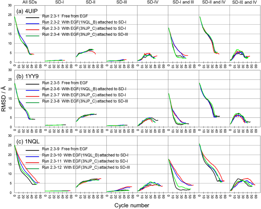
Forward Adiabatic Mapping from the Tethered Form to the Extended Form

1NQL, 1YY9 and 4UIP were selected as the basic initial structures for the forward mapping. The A-chain of 3NJP (3NJP_A) was selected as the target structure.¹⁵⁾ We also assumed the initial structures with EGF attached to SD-I or -III. Furthermore, two forms of EGF, sandwiched between SD-I and -III in the extended form (the C- and D-chains of 3NJP/1IVO)^1,15) and attached to mainly SD-I in the tethered form (the B-chain of 1NQL),¹¹⁾ were considered. Thus, we prepared 12 runs as shown in Fig. 5.

Fig. 5. Forward Adiabatic Mapping from the Tethered to the Extended Forms

The leftmost, the 2nd left, the 3rd left, the 4th left, the 4th right, the 3rd right, the 2nd right and the rightmost frames of each graph show RMSD for all SDs, for SD-I, for SD-II, for SD-III, for SD-IV, for SD-I and -III, for SD-II and -IV, and for SD-III and -IV, respectively. Horizontal axis of each graph shows cycle number every frame. (a), (b) and (c) show the mapping from 4UIP, 1YY9 and 1NQL, respectively. All runs are performed at pH 8.5. The RMSDs for SD-X (all SDs, SD-I, SD-II, SD-III, SD-IV, SD-I and -III, SD-II and -IV, or SD-III and -IV) are calculated after fitting only the corresponding SD-X. (Color figure can be accessed in the online version.)

Runs of 4UIP (Fig. 5a) and 1YY9 (Fig. 5b) showed very similar profiles to each other. For all SDs, these runs rapidly decreased RMSD in the initial stage, slowly decreased RMSD in the middle stage, rapidly decreased RMSD again in the final stage, and reached the minimal RMSDs of approximately 5 Å by the 40th cycle (the leftmost frame in Figs. 5a and 5b). The intradomain geometry of the SD-I and -III backbone was hardly changed (the 2nd and the 4th left frames in Figs. 5a and 5b), whereas that of SD-II was away from the target in spite of the mapping to the target (the 3rd left frame in Figs. 5a and 5b). The intradomain geometry of the SD-IV backbone was away from the target until the 20th cycle and then came near the target again, but did not come nearer to the target than the initial structure (the 4th right frame in Figs. 5a and 5b). The relative positions of SD-I and -III showed different profiles between “free from EGF,” “with EGF attached to SD-III” (runs 2.3-1, 2.3-4, 2.3-5 and 2.3-8) and “with EGF attached to SD-I” (runs 2.3-2, 2.3-3, 2.3-6 and 2.3-7). The former runs rapidly decreased the RMSDs until the 20th cycle, but the latter runs slowly decreased the RMSDs even after the 10th cycle. The profile for the relative positions of SD-II and -IV (the 2nd right frame in Figs. 5a and 5b) was similar to that for all SDs. The relative positions of SD-III and -IV were away from the target until the 20th cycle and then came near to the target again (the rightmost frame in Figs. 5a and 5b).

The mapping of 1NQL (Fig. 5c) showed different characteristics from the other two in view of the variation of RMSD for all SDs and for SD-III and -IV by attachment of EGF (the leftmost and the 2nd right frames in Fig. 5c), but, except for the above points, it showed a roughly similar profile to the other two.

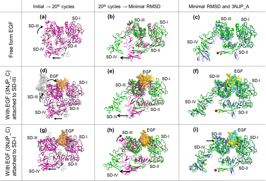
Representative structures in the forward mapping and their characteristics are shown in Fig. 6 and Table 4, respectively. The major geometrical different points between the tethered and the extended forms are the relative positions of SD-I and -III, and the distance between the hairpin loop in SD-II and the C-terminal tail of SD-IV. All runs tended to rearrange the relative position of SD-I and -III and to dissociate the C-terminal tail of SD-IV from the hairpin loop in SD-II (Figs. 6a, 6d and 6g). The runs “free from EGF” and “with EGF attached to SD-III” completed the rearrangement of SD-I and -III until the 20th cycle (Figs. 6b and 6e), but those “with EGF attached to SD-I” could not complete the rearrangement even after the 40th cycle (Figs. 6h and 6i, see the 3rd right frame in Figs. 5a, 5b and 5c). All runs needed more than 20 cycles to begin to dissociate the C-terminal tail of SD-IV from the hairpin loop in SD-II (Figs. 6b, 6e and 6h) and recovered the intradomain geometry of the SD-IV backbone to the initial/target structure after the dissociation, but did not recover the direction of the hairpin loop in SD-II (Figs. 6c, 6f and 6i).

Fig. 6. Examples of the ECD Conversion (PDB, 4UIP) from the Tethered to the Extended Forms (3NJP)

The ECDs are drawn in cartoon style, and EGFs are drawn in the surface style. The initial structures are colored grey. The 20th cycled structures are colored magenta for ECD and orange for EGF. The minimal RMSD structures are colored green for ECD and yellow for EGF. The target structures are colored blue for ECD and cyan for EGF. In the target structures, the Oη atom of Y251 (tip of the hairpin loop in SD-II) and the Nε atom of H566 (in SD-IV) are marked with red and yellow spheres, respectively. The two structures in each figure are fitted for SD-I. (Color figure can be accessed in the online version.)

Table 4. Characteristics of Structures Shown in Fig. 6

Initial structure	RMSDa)/Distance (Å)	The 20th cycle	Minimal RMSD
4UIP free from EGF	RMSD for “all SDs”	10.2	4.41
	RMSD for “SD-I and -III”	3.44	2.83
	RMSD for “SD-II and -IV”	14.4	5.26
	Distance between Y251Oη and H566Nε	4.70	27.7
	Distance between SD-I and -III	35.9	36.4
4UIP with EGF (3NJP_C) attached to SD-III	RMSD for “all SDs”	10.4	4.14
	RMSD for “SD-I and -III”	2.80	2.11
	RMSD for “SD-II and -IV”	15.0	5.47
	Distance between Y251Oη and H566Nε	5.42	28.4
	Distance between SD-I and -III	38.4	37.8
4UIP with EGF (3NJP_C) attached to SD-I	RMSD for “all SDs”	11.7	4.25
	RMSD for “SD-I and -III”	6.98	2.66
	RMSD for “SD-II and -IV”	14.7	5.41
	Distance between Y251Oη and H566Nε	6.03	26.5
	Distance between SD-I and -III	47.6	40.6

a) The RMSDs for SD-X (X = “all SDs,” “I and -III” or “II and IV”) were calculated after fitting for only corresponding SD-X.

We performed hinge analysis among the initial, the 20th cycle and minimum RMSD of 4UIP (Table 5 and Figure S1) by using the Hingefind algorithm.³⁸⁾ From a comparison between the initial and the 20th cycle of runs 2.3-1, 2.3-3 and 2.3-4, the hinge angle was the maximum between the 2nd and the 3rd subdomains (113.2° in run 2.3-1, 94.0° in run 2.3-3 and 115.1° in run 2.3-4). In contrast, from a comparison between the 20th cycle and the RMSD minimum of runs 2.3-1, 2.3-3 and 2.3-4, the hinge angle was the maximum between the 2nd last and the last subdomains (49.2° in run 2.3-1, 31.2° in run 2.3-3 and 48.1° in run 2.3-4).

Table 5. Hinge Angle Calculated by the Hingefind Algorithm

	Initial → 20th cycle				20th cycle → RMSD minimum
	Division	Rotation angle			Division	Rotation angle
4UIP free from EGF (run 2.3–1)	1–228, 235–236	10.9			1–241, 259–295, 299–483,487–500	49.2
	229–234, 237–244, 255–308		113.2
	309–504, 510–512			27.7
	247–252, 505–509, 513–572, 574–583, 587–593				484–486, 501–572, 574, 584–585, 587, 590–595
4UIP with EGF (3NJP_C) attached to D-III (run 2.3–3)	1–229, 234–238	11.0			1–228, 234–237	12.7
	230–233, 239–243, 255–308		94.0		229–233, 238–310		23.9
	309–504, 508–513			28.1	311–500, 503, 509			31.2
	505–507, 514–572, 575–576, 581–583, 587–593				501–502, 504–508, 510–571, 576, 582–583, 590–593
4UIP with EGF (3NJP_C) attached to SD-I (run 2.3–4)	1–228	16.6			1–484, 486–501	48.1
	229–243, 256–306		115.1
	309–503, 509–512			41.5
	504–508, 513–570, 581–582, 587–593				485, 502–571, 576–577, 580–583, 590–593

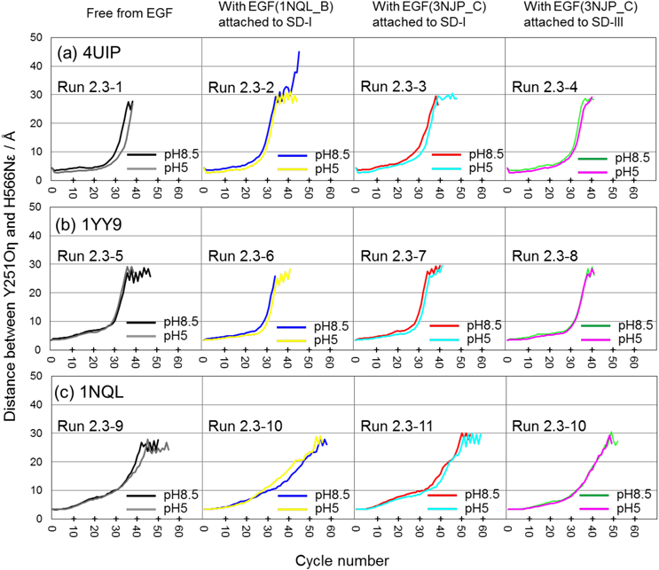
Ferguson et al. reported that in the presence of EGF, the dissociation of the hairpin loop in SD-II from the C-terminal tail of SD-IV is more suppressed at pH 5 than at pH 8.5, and this difference is related to the protonation of H566 in SD-IV.¹¹⁾ Hence, we performed 12 runs at pH 5 from the initial structures shown in Fig. 5. All runs at pH 5 of the 4UIP based initial structure showed a slightly slower dissociation than at pH 8.5 (Fig. 7a). However, two runs of the 1YY9-based initial structure [“free from EGF” (the leftmost frame of Fig. 7b) and “with EGF (3NJP_C) attached to SD-III” (the rightmost frame of Fig. 7b)], and two runs of the 1NQL-based initial structure [“with EGF (1NQL_B) attached to SD-I” (the 2nd left frame of Fig. 7c) and “with EGF (3NJP_C) attached to SD-III” (the rightmost frame of Fig. 7c)] did not.

Fig. 7. Adiabatic Mapping from the Tethered Form to the Extended Form at pH 5

The leftmost, the 2nd left, the 2nd right and the rightmost frames of each graph show “EGF free,” “with EGF (1NQL_B) attached to SD-I,” “with EGF (3NJP_C) attached to SD-I” and “with EGF (3NJP_C) attached to SD-III,” respectively. Vertical axis shows distance between Oη atom of Y251 (in SD-II) and Nε atom of H566 (in SD-IV). Horizontal axis of each graph shows cycle number for every frame. (a), (b) and (c) show the mapping from 4UIP, 1YY9 and 1NQL, respectively. (Color figure can be accessed in the online version.)

Reverse Adiabatic Mapping from the Extended Form to the Tethered Form

The A- and B-chains of 3NJP (3NJP_A and 3NJP_B), in which all SDs were preserved, were selected as the basic initial structures for the reverse mapping, and 4UIP was selected as the target structure because it had an average relative position of SD-I and -III in the tethered forms. The extended forms both “free from EGF” and “with EGF” (3NJP_C/3NJP_D) were assumed. The reverse mapping of the initial structures “free from EGF” (runs 2.4-1 and 2.4-2 in Fig. 8) had very similar profiles, and so did that of the initial structures “with EGF” (runs 2.4-3 and 2.4-4 in Fig. 8). The former runs rapidly decreased RMSD for all SDs (the leftmost frame in Fig. 8) until the 20th cycle and then remained almost flat at RMSD of approximately 9 Å, whereas the latter runs decreased RMSD slower for all SDs after the 10th cycle than the former runs, and did not become flat even after the 40th cycle (the leftmost frame in Fig. 8). The intradomain geometry of the SD-I and -III backbone was hardly changed (the 2nd and the 4th left frames in Fig. 8), whereas that of the SD-II and -IV backbone was away from the target in spite of the mapping to the target (the 3rd left and the 4th right frames in Fig. 8). The relative positions of SD-I and -III showed different profiles between “free from EGF” (runs 2.4-1 and 2.4-2) and “with EGF” (runs 2.4-3 and 2.4-4). The former runs rapidly decreased RMSD for SD-I and -III until the 20th cycle and remained almost flat at RMSD less than 8.5 Å, whereas the latter runs decreased RMSD for SD-I and -III slower than the former runs from the first stage, and did not become flat even after the 40th cycle (the 3rd right frame in Fig. 8). All runs rapidly decreased RMSD for SD-II and -IV until the 20th cycle, and after that, remained flat at RMSD of approximately 8 Å (the 2nd right frame in Fig. 8). All runs showed the relative position of SD-III and -IV away from the target until the 20th cycle, and then was roughly constant, but the flat level was different between “free from EGF” (runs 2.4-1 and 2.4-2, RMSD of approximately 6.5 Å) and “with EGF” (runs 2.4-3 and 2.4-4, RMSD of 8.5-10 Å) (the rightmost frame in Fig. 8).

Fig. 8. Reverse Adiabatic Mapping from the Extended to the Tethered Forms

The leftmost, the 2nd left, the 3rd left, the 4th left, the 4th right, the 3rd right, the 2nd right and the rightmost frames of each graph show RMSD for all SDs, for SD-I, for SD-II, for SD-III, for SD-IVI, for SD-I and -III, for SD-II and -IV, and for SD-III and -IV, respectively. Horizontal axis of each graph shows cycle number for every frame. All runs are performed at pH 8.5. The RMSDs for SD-X (all SDs, -I, -II, -III, -IV, -I and -III, -II and -IV or -III and -IV) are calculated after fitting only the corresponding SD-X. (Color figure can be accessed in the online version.)

Examples of the reverse mapping are shown in Fig. 9. All runs achieved the association of the C-terminal tail of SD-IV to the hairpin loop in SD-II. Two runs “free from EGF” (runs 2.4-1 and 2.4-2) rearranged the relative position of SD-I and -III at the same time (Fig. 9a), but the other runs (“with EGF,” runs 2.4-3 and 2.4-4) did not complete the rearrangement even after the 40th cycle (Figs. 9b and 9c).

Fig. 9. Examples of the ECD Transition from the Extended Form (3NJP_A) to the Tethered Form (4UIP_A, Grey)

(a) The 18th cycled structure (magenta) in the mapping from the initial structure free from EGF. (b) The 18th cycled structure (cyan) in the mapping from the initial structure with EGF (orange). (c) The 40th cycled structure (green) in the mapping from the initial structure with EGF (yellow). Each cycled structure is fitted on the target (4UIP_A) for SD-I and -III. The two structures in each figure are fitted for SD-I and -III. (Color figure can be accessed in the online version.)

Discussion

The comparison among six tethered forms revealed the rigidity of the intradomain geometry of the SD-I and -III backbone, the variation of the intradomain geometry of the SD-II backbone and the deviation of the relative position of SD-I and -III. These results suggest that the intradomain geometry of the SD-II backbone is flexible and it influences the relative positions of SD-I and -III. Adiabatic mapping among the tethered forms complemented the above proposition, that is, the mapping rearranged the relative positions of SD-I and -III but did not change the intradomain geometry of the SD-I and -III backbone. The lowest frequency normal modes mainly contributed to the rearrangement, which suggested that the mode is a strong driving force to change the relative positions of SD-I and -III in the tethered form.

The ECD conversion from the tethered to the extend forms is very dynamic and complicated, and the process has not yet been clarified. In this study, we performed adiabatic mapping between the tethered and the extend forms to obtain further insight. First, the intradomain geometry of SD-I and -III backbone was shown to be rigid from the two-way mapping (the 2nd and 4th left frames in Figs. 5 and 8). Second, the geometry of the tethered form had two potential driving forces to rearrange the relative positions of SD-I and -III and to dissociate the C-terminal tail of SD-IV from the hairpin loop in SD-II (Figs. 6a, 6d and 6g).

The forward mapping of the initial structures free from EGF smoothly rearranged the relative positions of SD-I and -III (the 3rd right frame in Figs. 5 and 6a), whereas that with EGF attached to SD-I hardly did (the 3rd right frame in Figs. 5 and 6g). These results showed that the EGF attachment to SD-I of the tethered form disturbed the rearrangement of SD-I and -III to convert to the extended form. However, the forward mapping of the initial structures with EGF attached to SD-III rearranged the relative positions of SD-I and -III as smoothly as those free from EGF (the 3rd right frame in Figs. 5 and 6d). This unexpected result suggests that the EGF attachment to SD-III of the tethered form does not disturb the relative position rearrangement of SD-I and -III. It has long been discussed whether EGF attaches to SD-I or -III in the ECD conversion. Loeffler and Winn argued for a preceding EGF attachment to SD-III from the viewpoint of free energy when binding at physiological pH.¹⁹⁾ Ferguson et al. identified the crystal structure of ECD, in which EGF mainly attached to SD-I at pH 5, and argued that low pH (such as at pH 5) made EGF attachment to SD-I more advantageous than to SD-III because the protonation of residues in SD-I strengthened the binding to EGF. In contrast, SD-III seemed not to be influenced by pH because the main driving force to bind to EGF is a hydrophobic interaction.¹¹⁾ The above discussions suggest that SD-III binds to EGF more readily than SD-I at physiological pH. Our study revealed that the EGF attachment to SD-III was geometrically more advantageous than SD-I because the EGF attachment position to SD-III does not disturb the conversion from the tethered form to the extended form.

The dissociation of the C-terminal tail of SD-IV from the hairpin loop in SD-II is also an important factor for the tethered form to be converted to the extended form as well as the relative position rearrangements of SD-I and -III. All runs of the forward mapping exhibited the dissociation trend, but needed more than 20 cycles until the dissociation began. Until the 20th cycle, the hairpin loop in SD-II bent as if it was pulled by the C-terminal tail of SD-IV, and then they both began to dissociate (Figs. 6b, 6e, 6h). Lowering the pH (8.5 → 5) is known to restrain the conversion of the tethered form to the extended form in the presence of EGF, and the protonation of H566 is considered to be associated with this restraint.^11,17) We also performed the forward mapping from the tethered to the extended forms at low pH (pH = 5, Fig. 7). However, all initial structures did not express a significant restraint by lowering the pH, although some runs showed a slight delay of dissociation (therefore we judged the delay as “not significant”). ENM-NMA used in this study handles only heavy atoms and considers all interatomic interactions as harmonic oscillators, like springs, but does not distinguish between electrostatic interactions (repulsive and attracting forces) because it neglects atomic charge. To compensate for this defect, we introduced energy optimization using AMBER Force Fields,³⁹⁾ but this method may be insufficient to express the mapping that considers electrostatic interactions.

The aim of the reverse adiabatic mapping (from the extended to the tethered forms) was to clarify if the extended form could return to the tethered form. The reverse mapping “free from EGF” rapidly rearranged the relative positions of SD-I and -III (Figs. 8 and 9a), whereas that “with EGF” hardly rearranged the relative positions owing to the EGF attachment to both SD-I and -III (Figs. 8, 9b and 9c). The latter result suggests that the extended form “with EGF” sandwiched between SD-I and -III was unlikely to return to the tethered form and complements the finding that EGF promotes the ECD conversion from the tethered to the extended forms. However, the reverse mapping “free from EGF” did not reach the target (RMSD of approximately 9 Å for all SDs, the leftmost frame in Fig. 8) as well as the forward mapping from the tethered to the extended forms (RMSD of approximately 5 Å for all SDs, Fig. 5). Especially, the intradomain geometry of the SD-II and -IV backbone and the relative positions of SD-III and -IV were farther from the target than the initial structure (the leftmost, the 3rd left, the 4th right and the rightmost frames in Fig. 8). In this study, we combined EMN-NMA and energy optimization using a molecular force field and obtained some insights about the ECD conversion, but better mapping may be possible by setting the parameters of ENM-NMA or introducing short molecular dynamics calculations.

Conclusion

We compared the X-ray crystal structures of ECD and simulated the ECD conversion between the two forms by adiabatic mapping combining ENM-NMA and energy optimization. The mapping among the tethered forms well expressed the relative position variations of SD-I and -III observed by comparing the X-ray crystal structures, and the lowest frequency normal mode mainly contributed to the variation. The forward mapping from the tethered to the extended forms showed the rigidity of the intradomain geometry of the SD-I and -III backbone and two trends to rearrange the relative position of SD-I and -III and to dissociate the C-terminal tail of SD-IV from the hairpin loop in SD-II. EGF attached to SD-I of the tethered form disturbed the relative position rearrangements of SD-I and -III to convert to the extended form, whereas EGF attached to SD-III unexpectedly did not disturb this rearrangement. The reverse mapping from the extended to the tethered forms suggested that the extended form with EGF sandwiched between SD-I and -III does not return to the tethered form, and complemented the promotion of the ECD conversion under the presence of EGF. Our method, however, could not clarify the difference between pH (8.5 and 5), and there may a possibility for better mapping.

Experimental

ENM-NMA

In this study, we adopted a new ENM-NMA method developed by Lu and Ma, known as the molecular geometry restraints (MGR) method.³²⁾ This method does not treat “bonded” and “non-bonded” as having the same potential function, unlike conventional ENM, but provides three restraining terms on the molecular geometry of “bonded,” that is, bond length, bond angle and dihedral angle. Consequently, the potential function used in the MGR method has four terms:

  

(1)

Each potential term of MGR is a harmonic potential with an energy minimum on the initial (X-ray crystal) structure. The first three terms, V_bond, V_angle and V_dihedral, denote bond length, bond angle and dihedral angle potentials, respectively, and are adopted when two atoms are covalently bound. They have forms of

  

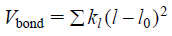(2)

where the summation is over all covalent bonds, l and l₀ are the instantaneous and initial bond lengths, k_l is the force constant;

  

(3)

where the summation is over all bond angles, θ and θ₀ are the instantaneous and initial bond angles, k_θ is the force constant; and

  

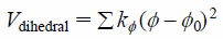(4)

where the summation is over all dihedral angles and improper dihedral angles, ϕ and ϕ₀ are the instantaneous and initial dihedral angles, k_ϕ is the force constant. The last term V_non-bond denotes a non-covalent bond potential in the form of

  

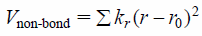(5)

where r and r₀ are the instantaneous and initial distances between two non-covalent bond atoms, k_r is the force constant but is weighted by the following term.²⁵⁾

  

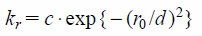(6)

where c is set as 1 kcal·mol⁻¹ Å⁻¹. The exponential decay allows the evaluation with a cutoff not significantly larger than the distance d, and d was set as 3 Å.²⁵⁾ The cutoff distance of r₀ applied to Eq. (5) was chosen as 10 Å. The force constants of k_l, k_θ and k_ϕ were set as 1.0 × 10⁴ kcal·mol⁻¹ Å⁻¹, 820 and 62 kcal·mol⁻¹ degree ⁻¹, respectively.³²⁾

We used a program for NMA, PDBMAT, downloaded from the web-interface elNémo.²⁷⁾ The coordinates of only the heavy atoms were used for the NMA calculation because the H atom-added system was too large to calculate the matrix using our machines. The heavy atoms used in this study were carbon, nitrogen, oxygen and sulfur. To simplify the calculation of the system, masses of the heavy atoms were unified. The fluctuation profile calculated by the MGR method was very similar to that estimated from the B-factor except for the C-terminal (Fig. S2). The deviation of the C-terminal was because the calculation by the MGR method neglects missing residues (residue 615–621).¹⁵⁾ The disordered residues may contribute to the fluctuation damping of the C-terminal tail of SD-IV by intermolecular interaction. Thus we confirmed that the MGR method adequately expressed the collective motion of ECD.

Adiabatic Mapping

We performed adiabatic mapping by combining ENM-NMA and energy optimization using molecular force fields. The procedure was as follows;

i) ENM-NMA was performed for the initial structure, and ten low frequency normal modes were extracted.

ii) The initial structure was moved to the target linearly along the ten modes according to the following expressions.

  

(7)

where p⁰ is the initial structure, p¹_k is the structure after moving along the k-th normal mode in the 1st cycle, a¹_k is an eigenvector of the k-th normal mode with an eigenvalue ω_k in the 1st cycle. k takes a value within the range of 1 ≤ k ≤ 10, 1 is the lowest frequency normal mode, 2 is the 2nd lowest frequency normal mode, ……, 9 is the 9th lowest frequency normal mode and 10 is the 10th lowest frequency normal mode. A coefficient x regulates the movement step, and in this study, the value was set to 0.5. The calculated a_k is expressed as a unidirectional vector (+), and may be used as the adverse vector (−). Whether to be used as “unidirectional (+),” or “the adverse (−)” was judged by RMSD between the structure after moving and the target, and the direction whose RMSD was smaller was adopted.

iii) The moved structure p¹₁₀ may have a distorted structure by procedure ii). Furthermore, ENM-NMA does not consider the charge state of the molecule. To solve these two problems, energy optimization was performed for p¹₁₀. The optimization was performed using the SANDER of AMBER (version 14) with an all-atom Amber99SB force field and the implicit solvent method.³⁹⁾ The generalized Born (GB) solvation model was used as the implicit solvent model.^40,41) To avoid destruction of the form, the optimization was performed in two stages, the 1st optimization (with position restraint) and the 2nd optimization (without position restraint). The optimization was performed for pH 5 and pH 8.5. The charge state of pH 5 and pH 8.5 was decided by referencing the report by Dong et al.¹⁷⁾

iv) For the moved structure, i), ii) and -III) was repeated until the minimal RMSD for all SDs was reached. In the n-th cycle, expressions (8) are as follows;

  

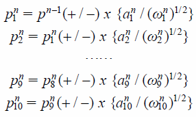(8)

where pⁿ⁻¹ is the energy-optimized coordinates after the (n − 1)-th cycle, pⁿ_k are the coordinates after moving along the k-th normal mode in the n-th cycle, a¹_k is an eigenvector of the k-th normal mode with an eigenvalue ωk in the n-th cycle. The other descriptors are the same as those in expressions (7).

Acknowledgments

We would like to thank Dr. Kazuhiko Kanou, Dr. Kensyu Kamiya, Dr. Hiromitsu Shimoyama, Chiaki Tashiro, Tomomi Kakuta, Hazuki Sato and Arisa Yamamoto for their support and helpful discussions. For calculation of the superposition and creation of graphics, we used the graphics software, PyMOL, a molecular visualization system on an open-source foundation, maintained and distributed by Schrödinger, Inc. (New York, U.S.A.).

Conflict of Interest

The authors declare no conflict of interest.

Supplementary Materials

The online version of this article contains supplementary materials.

References

• 1) Ogiso H., Ishitani R., Nureki O., Fukai S., Yamanaka M., Kim J. H., Saito K., Sakamoto A., Inoue M., Shirouzu M., Yokoyama S., Cell, 110, 775–787 (2002).
• 2) Dawson J. P., Bu Z., Lemmon M. A., Structure, 15, 942–954 (2007).
• 3) Garrett T. P., McKern N. M., Lou M., Elleman T. C., Adams T. E., Lovrecz G. O., Zhu H. J., Walker F., Frenkel M. J., Hoyne P. A., Jorissen R. N., Nice E. C., Burgess A. W., Ward C. W., Cell, 110, 763–773 (2002).
• 4) Yun C. H., Boggon T. J., Li Y., Woo M. S., Greulich H., Meyerson M., Eck M. J., Cancer Cell, 11, 217–227 (2007).
• 5) Park J. H., Liu Y., Lemmon M. A., Radhakrishnan R., Biochem. J., 448, 417–423 (2012).
• 6) Solca F., Dahl G., Zoephel A., Bader G., Sanderson M., Klein C., Kraemer O., Himmelsbach F., Haaksma E., Adolf G. R., J. Pharmacol. Exp. Ther., 343, 342–350 (2012).
• 7) Yosaatmadja Y., Silva S., Dickson J. M., Patterson A. V., Smaill J. B., Flanagan J. U., McKeage M. J., Squire C. J., J. Struct. Biol., 192, 539–544 (2015).
• 8) Li S., Schmitz K. R., Jeffrey P. D., Wiltzius J. J., Kussie P., Ferguson K. M., Cancer Cell, 7, 301–311 (2005).
• 9) Schmitz K. R., Bagchi A., Roovers R. C., van Bergen en Henegouwen P. M., Ferguson K. M., Structure, 21, 1214–1224 (2013).
• 10) Sickmier E. A., Kurzeja R. J., Michelsen K., Vazir M., Yang E., Tasker A. S., PLOS ONE, 11, e0163366 (2016).
• 11) Ferguson K. M., Berger M. B., Mendrola J. M., Cho H. S., Leahy D. J., Lemmon M. A., Mol. Cell, 11, 507–517 (2003).
• 12) Ramamurthy V., Krystek S. R. Jr., Bush A., et al., Structure, 20, 259–269 (2012).
• 13) Lee J. J., Choi H. J., Yun M., Kang Y., Jung J. E., Ryu Y., Kim T. Y., Cha Y. J., Cho H. S., Min J. J., Chung C. W., Kim H. S., Angew. Chem. Int. Ed., 54, 12020–12024 (2015).
• 14) Lim Y., Yoo J., Kim M. S., et al., Mol. Cancer Ther., 15, 251–263 (2016).
• 15) Lu C., Mi L. Z., Grey M. J., Zhu J., Graef E., Yokoyama S., Springer T. A., Mol. Cell. Biol., 30, 5432–5443 (2010).
• 16) Arkhipov A., Shan Y., Das R., Endres N. F., Eastwood M. P., Wemmer D. E., Kuriyan J., Shaw D. E., Cell, 152, 557–569 (2013).
• 17) Dong J., Zhang Y., Zhang Z., J. Mol. Model., 22, 131 (2016).
• 18) Du Y., Yang H., Xu Y., Cang X., Luo C., Mao Y., Wang Y., Qin G., Luo X., Jiang H., J. Am. Chem. Soc., 134, 6720–6731 (2012).
• 19) Loeffler H. H., Winn M. D., Proteins, 81, 1931–1943 (2013).
• 20) Nojima H., Takeda-Shitaka M., Kurihara Y., Adachi M., Yoneda S., Kamiya K., Umeyama H., Chem. Pharm. Bull., 50, 1209–1214 (2002).
• 21) Nojima H., Takeda-Shitaka M., Kurihara Y., Kamiya K., Umeyama H., Chem. Pharm. Bull., 51, 923–928 (2003).
• 22) Nojima H., Takeda-Shitaka M., Kanou K., Kamiya K., Umeyama H., Chem. Pharm. Bull., 56, 635–641 (2008).
• 23) Nojima H., Kanou K., Kamiya K., Atsuda K., Umeyama H., Takeda-Shitaka M., Chem. Pharm. Bull., 57, 1193–1199 (2009).
• 24) Tirion M. M., Phys. Rev. Lett., 77, 1905–1908 (1996).
• 25) Bahar I., Atilgan A. R., Erman B., Fold. Des., 2, 173–181 (1997).
• 26) Hinsen K., Proteins, 33, 417–429 (1998).
• 27) Tama F., Sanejouand Y. H., Protein Eng., 14, 1–6 (2001).
• 28) Suhre K., Sanejouand Y.H. Nucleic. Acids. Res., 32, W610-4 (2004).
• 29) Delarue M., Sanejouand Y. H., J. Mol. Biol., 320, 1011–1024 (2002).
• 30) Valadié H., Lacapcre J. J., Sanejouand Y. H., Etchebest C., J. Mol. Biol., 332, 657–674 (2003).
• 31) Nicolay S., Sanejouand Y. H., Phys. Rev. Lett., 96, 078104 (2006).
• 32) Lu M., Ma J., Arch. Biochem. Biophys., 508, 64–71 (2011).
• 33) Na H., Song G., Proteins, 83, 273–283 (2015).
• 34) Wako H., Endo S., Biophys. Chem., 159, 257–266 (2011).
• 35) Wako H., Endo S., Comput. Biol. Chem., 44, 22–30 (2013).
• 36) Wako H., Endo S., Biophys. Rev., 9, 877–893 (2017).
• 37) Berman H. M., Westbrook J., Feng Z., Gilliland G., Bhat T. N., Weissig H., Shindyalov I. N., Bourne P. E., Nucleic Acids Res., 28, 235–242 (2000).
• 38) Wriggers W., Schulten K., Proteins, 29, 1–14 (1997).
• 39) Hornak V., Abel R., Okur A., Strockbine B., Roitberg A., Simmerling C., Proteins, 65, 712–725 (2006).
• 40) Bashford D., Case D. A., Annu. Rev. Phys. Chem., 51, 129–152 (2000).
• 41) Tsui V., Case D. A., Biopolymers, 56, 275–291 (2000–2001).