TRMM/GPM　Goddard潜熱推定アルゴリズム

Abstract

The Goddard Convective-Stratiform Heating (CSH) algorithm has been used to retrieve latent heating (LH) associated with clouds and cloud systems in support of the Tropical Rainfall Measuring Mission (TRMM) and Global Precipitation Measurement (GPM) mission. The CSH algorithm requires the use of a cloud-resolving model (CRM) to simulate LH profiles to build look-up tables. This paper describes the current V6 CSH and its differences/similarities versus the previous V5 CSH. Long-term CRM simulations were conducted to identify the impact of the CRM resolution and convective-stratiform separation method on LH structure/profiles. The TRMM and GPM Combined radar-radiometer algorithm-derived surface rain rates and their associated precipitation properties were the input to the CSH algorithm.

CSH V6-retrieved regional LH profiles in the tropics and subtropics display the classic signatures of heating in the convective region and heating over cooling in the stratiform region. Because there is no direct measurement of LH structure, the performance of the CSH V6 algorithm is examined by comparing its vertically integrated heating (or equivalent surface rain rate) against the surface rain rate derived from the TRMM/GPM Combined algorithm. The CSH three-month and zonal mean equivalent surface rain rates are in good agreement with the Combined rain rates over the Inter Tropical Convergence Zone region; the agreement is best over the ocean. CSH three-month and zonal mean equivalent surface rain rates are larger than the Combined rain rates over land in both the tropics and subtropics. CSH three-month mean equivalent surface rain rates also have local differences with the Combined rain rates that can be smoothed by area averaging to larger horizontal resolutions (from the CSH standard grid of 0.25° × 0.25° to 0.5° × 0.5° or 1.0° × 1.0°). CSH equivalent surface rain rates have more light rain rates but less larger rates compared to the GPM Combined surface rain rates.

1. Introduction

Latent heat release via precipitation formation is a primary driver of large- and small-scale atmospheric circulations, particularly in the tropics where various large-scale tropical modes dominated by latent heating (LH) persist and vary on a global scale. LH and its variation are among the most important physical processes within the atmosphere and are central to Earth's water and energy cycle. LH release is caused by the phase changes in water between its vapor, liquid, and solid states, namely, condensation, evaporation, deposition, sublimation, melting, and freezing. Latent heat release is dominated by condensation and deposition, and heat absorption by evaporation and sublimation. Heat absorption by melting occurs near the 0.0°C level. The melting process is important because precipitating ice particles melt into raindrops before reaching the ground as surface rainfall. The heat released via freezing is smaller than that of condensation and deposition but is still important for microphysical processes (Figs. 7, 8 in Tao et al. 1990).

The Tropical Rainfall Measuring Mission satellite (TRMM, Simpson et al. 1988) made quantitative measurements of tropical rainfall on a continuous basis over the global tropics, which were then used to estimate the four-dimensional (4D) structure of LH over the global tropics (Simpson et al. 1996). Standard LH products from TRMM measurements have been established as a valuable resource for scientific research and applications (see review papers by Tao et al. 2006, 2016a). Such products enable new insights and investigations into the complexities of convective system life cycles, diabatic heating controls and feedbacks related to meso- and synoptic-scale circulations and their prediction, and the relationship between tropical LH patterns and the global circulation. TRMM's success provided the impetus for another major international satellite mission known as the Global Precipitation Measurement (GPM; Hou et al. 2014; Skofronick-Jackson et al. 2017; Nakamura 2021). As the centerpiece of NASA's Weather and Global Water/Energy Cycle research programs, GPM is providing the next-generation of space-borne precipitation measurements. It covers a broader area (from the tropics to higher latitudes) relative to TRMM, and its dual-frequency Ku–Ka band radar (DPR; Kojima et al. 2012) on the core observatory provides higher accuracy precipitation measurements.

LH cannot be measured directly with current techniques, including current remote sensing or in situ instruments. Therefore, cloud-resolving models (CRMs) play a critical tool in establishing the quantitative and physical relationships between diabatic heating and rainfall. CRMs have sophisticated microphysics schemes (that are by no means perfect) that can reasonably simulate cloud and precipitation processes and their explicit interactions with the surface and radiation (see a review by Tao and Moncrieff 2009). CRM-simulated data have, in fact, been used extensively to develop rain and LH retrieval algorithms for TRMM. Regional-scale models (with domains of several hundred to several thousand km²) are also indispensable tools. They are extremely flexible and allow for a wide range of horizontal resolutions (via nesting), a variety of physical processes, and the realistic representation of topography, precipitation processes, land surface–atmosphere hydrology, and energy coupling (including realistic vegetation/soil interaction and atmospheric planetary boundary layer processes). They can be nested to resolve convection and thereby use the same microphysics as CRMs. Both CRMs and regional-scale models are important to GPM-algorithm developers and are considered key components of one of the major GPM ground validation (GV) sites (see GPM GV document, https://gpm.nasa.gov/category/major-category/science?page=5).

Currently, there are two standard TRMM/GPM LH algorithms, namely, the Goddard Convective-Stratiform Heating (CSH) and Japan Spectral Latent Heating (SLH). Both depend on CRM simulations (i.e., from the Goddard Cumulus Ensemble model or GCE) and regional-scale models (i.e., the NASA Unified Weather Research and Forecasting model or NU-WRF and the Japan Meteorological Agency's Local Forecast Model or LFM) for their look-up tables (LUTs).

Because there is no direct measurement of LH, Tao et al. (1990) used results from the GCE model to develop the first LH algorithm. However, this algorithm requires specific coefficients related to cloud (cloud ice) to estimate condensation (deposition) heating. Therefore, Tao et al. (1993) proposed a second LH algorithm (the CSH algorithm) as LH profiles are quite different between the convective and stratiform regions (Houze 1982, 1997; Johnson 1984; Johnson and Young 1983). The CSH algorithm's performance was tested through self-consistency checking using GCE-simulated LH data as “truth” (Tao et al. 2000), and the algorithm was used to retrieve LH structures using one-month of TRMM rainfall products (Tao et al. 2001). Later, the CSH algorithm was redesigned and improved by using several long-term GCE simulations and differentiating the LUTs into many bins and into separate heating components (Tao et al. 2010). In Tao et al. (2010), the number of LH profiles in the CSH LUTs (i.e., ocean and land) is greatly increased (∼ 36 intensity and 20 stratiform bins) versus the previous version (i.e., Tao et al. 1993, 2000, 2001). In addition, the profiles are binned according to the mean conditional surface rain rates obtained from the GCE model subdomains roughly consistent with the size of the CSH LH product grids (i.e., 64 km model subdomains are used to build the LUTs for the TRMM half degree gridded products). Recently, the CSH algorithm was revised again (Lang and Tao 2018). In addition to conditional surface rain intensities and stratiform fraction, the land and ocean LUTs are further binned according to the mean echo-top heights and low-level vertical reflectivity gradients (downward increasing or decreasing) to improve the depth of heating and intensity of low-level evaporative cooling in stratiform regions, respectively. The GCE CRM database from which the CSH LUTs are derived was also upgraded with additional cases and the use of the improved Goddard 4ICE scheme (Lang et al. 2014; Tao et al. 2016). Tao et al. (2019) used NU-WRF-simulated precipitation properties to produce high latitude or cold season's LUTs for the CSH algorithm. Please see Table 1, which lists the highlights and references for the CSH algorithm over the course of its continued development.

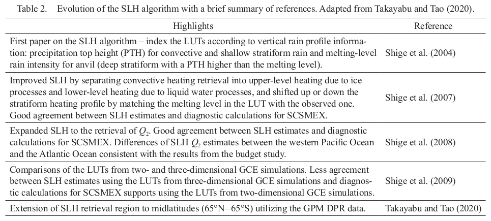
Table 2 shows a brief summary of the evolution of the SLH algorithm described in Shige et al. (2004, 2007, 2008, 2009). SLH LUTs are also generated from the GCE model as with the CSH algorithm. Deep stratiform rain is further divided into two new categories: deep stratiform with decreasing precipitation from the melting level toward the surface (downward decreasing: DD) and deep stratiform with increasing precipitation from the melting level toward the surface (downward increasing: DI). Similar categories are already applied in the CSH algorithm. The SLH algorithm computes deep stratiform cooling magnitudes as a function of Pm (melting level) – Ps (surface rain rate), assuming that the evaporative cooling rate below the melting level in deep stratiform regions is proportional to the reduction in the precipitation profile toward the surface from the melting level [based on one-dimensional (or 1D) water substance conservation]. However, increasing precipitation profiles are found in some portions of stratiform regions, especially in regions adjacent to convective regions where 1D water substance conservation may be invalid. A LUT for deep stratiform with increasing precipitation toward the surface from the melting level (called “intermediate”) is produced with the amplitude determined by Ps. Please also see Takayabu and Tao (2020) for the SLH-derived LH structures.

The objective of the paper is to describe the current Goddard CSH algorithm, including the improvements and similarities/differences from the previous version (Tao et al. 2010; Lang and Tao 2018), and to examine its performance using GPM Combined radar-radiometer algorithm (or Combined algorithm hereafter; Grecu et al. 2016)-derived surface rain rates. The algorithm description and its improvements are presented in Section 2. In Section 3, the impact of some improvements to the CSH algorithm will be investigated via GCE model sensitivity tests. The CSH-retrieved LH structures and their associated performance are shown in Section 4. The conclusions and future work are presented in Section 5.

2. Algorithm description

2.1 Differences and similarities between the current V6 and previous V5 CSH algorithms

For the current V6 CSH algorithm, the Level 2 pixel product (named 2HCSH) is the primary CSH product, with the V6 Level 3 gridded product (3GCSH) merely an aggregation of the V6 Level 2 pixel product. Figure 1 shows a schematic diagram of the CSH V6 algorithm for both TRMM and GPM. It consists of a warm season component using GCE model-generated LUTs and a cold season component using NU-WRF-generated LUTs. Table 3 shows the similarities and differences between CSH V5 and V6. There are two major changes that have affected the retrieved CSH LH on the GPM grid. The first one is the change in LUTs from gridded (0.25° × 0.25° − Level 3) to pixel (4 km − Level 2). The second is due to the change in the convective-stratiform separation method. This second change was made to make the separation more consistent with the satellite method. The input to the CSH V6 algorithm consists of the surface precipitation derived from the V08 and V06 of the TRMM and GPM Combined algorithm, respectively, as well as its classification (convective or stratiform) and various associated radar characteristics (e.g., echo-top height).

Fig. 1.

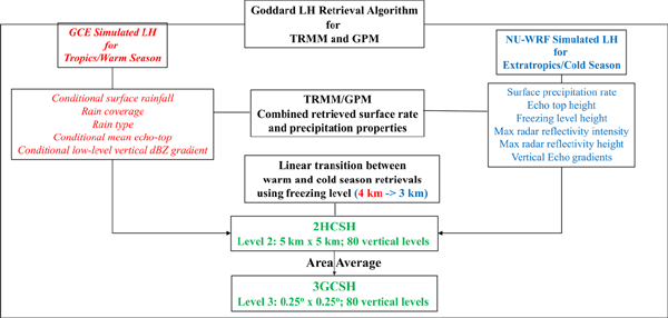
Schematic diagram of the Goddard CSH retrieval algorithm for TRMM and GPM.

a. Warm season – tropical

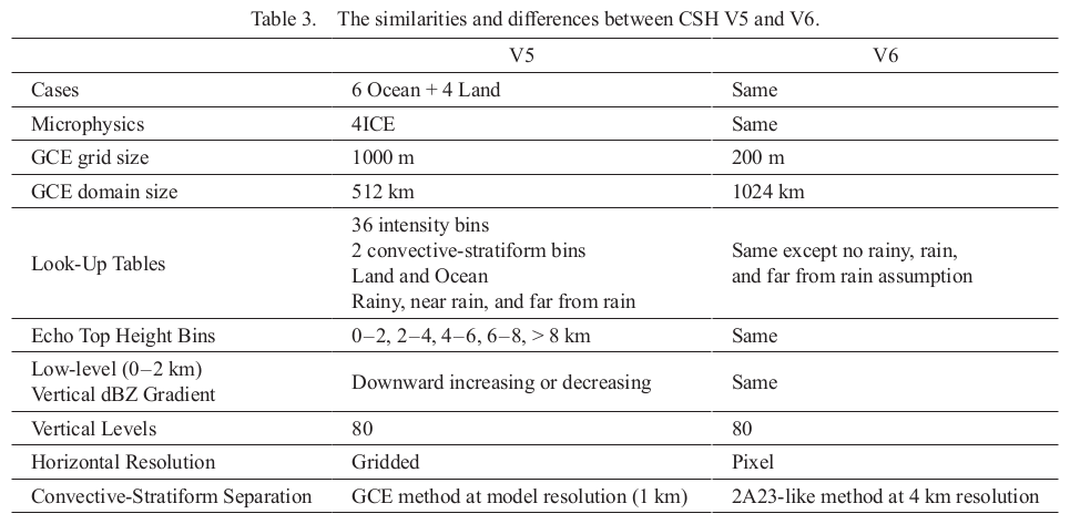
For the 2HCSH pixel product, mean heating profiles from the GCE model are averaged over 4 km GCE subdomains (roughly consistent with the DPR surface pixel size) and are then binned according to the mean surface rain rate and to whether the subdomain is convective or stratiform. In addition to the 36 surface rain intensity bins (every 20 mm day⁻¹) and convective and stratiform bins, the CSH LUTs are further binned according to the mean echo-top height (5 bins, 0–2, 2–4, 4–6, 6–8, and > 8 km) and low-level (0–2 km above ground level, AGL) vertical reflectivity gradient (downward increasing or decreasing), which were introduced in the previous V5 algorithm (Lang and Tao 2018) to improve heating depth and intensity of low-level evaporative cooling in stratiform regions, respectively. For V6, the CSH LUTs are still composited into land and ocean regions. However, the “near rain” and “far from rain” LUTs are no longer used (i.e., LH is only retrieved for rainy pixels). The CSH land and ocean LUTs are still composited from six multiweek ocean cases and four multiweek land cases (see Table 2 in Lang and Tao 2018 and Tao et al. 2019).

The GCE is still run two-dimensionally (2D) using the improved one-moment Goddard four class (cloud ice, snow, graupel, and hail) ice (4ICE) cloud microphysics scheme (Lang et al. 2014; Tao et al. 2016b), which includes a bin microphysics-based rain evaporation correction. However, for V6, the GCE CSH LUT database is generated using a horizontal resolution of 200 m (versus 1000 m for V5) and a horizontal domain of 1024 km (versus 512 km for V5) to improve the simulation of shallow clouds and large mesoscale convective systems, respectively. The 200 m grid is averaged to 4 km for the LUTs and convective-stratiform separation. In addition, the V5 gridded product had 20 stratiform fraction bins (every 5 %) that are not needed for V6.

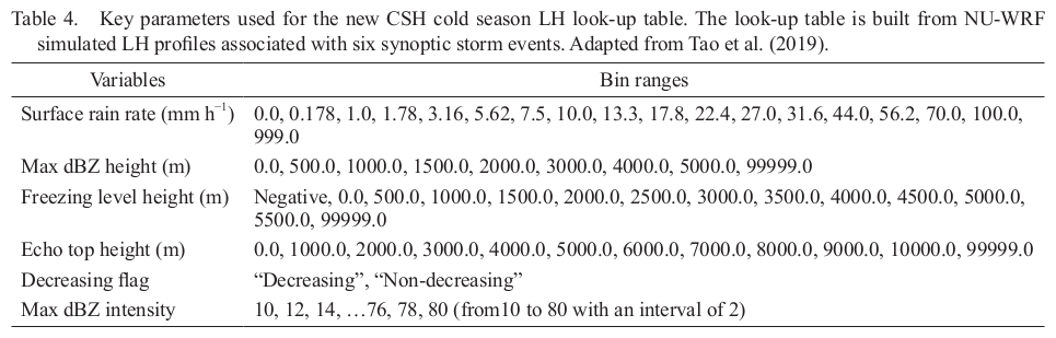
b. Cold Season – extratropics

LH profiles obtained from six NU-WRF simulations using the same improved 4ICE scheme for three eastern US synoptic snow storms and three West Coast atmospheric river events are mapped to the satellite using a similar but differing set of metrics than those used for the tropical/warm season algorithm (Tao et al. 2019).

The extratropical/cold season LUTs are constructed from the innermost, 3 km domain and mapped using the following metrics: storm top height (11 bins), freezing level (13 bins), max dBZ level (8 bins), and vertical dBZ gradient (2 bins). For V6, the number of bins for the first three metrics was increased, and a new metric (surface precipitation rate) was added with 17 bins. Heating intensity is based on the composite dBZ intensity. For V5, there were 90 bins every 1 dBZ, but for V6, the bin size was increased to every 2 dBZ with a slightly narrower range. Table 4 shows the metrics and corresponding bins used for the CSH V6 extratropical/cold season LH LUT. The bin ranges are based on the close examination of the NU-WRF simulation results.

As with V5, the CSH V6 cold and warm season heating retrievals are selected according to the height of the freezing level. When the freezing level is above 4 km, the warm season retrievals are used; when it is below 3 km, the cold season values are used. Between 3 km and 4 km, the cold and warm season values are averaged with a linear temperature weighting. For the satellite orbits, the freezing level height is obtained from the corresponding analysis [JMA global analysis (GANAL)] data.

2.2 Convective-stratiform separation methods

A major change for CSH V6 is the use of a convective-stratiform separation scheme that is more consistent with that applied to the GPM satellite data. The V6 separation method is now based on a Steiner-type method (Steiner et al. 1995) similar to the GPM method (named 2A23; see Awaka et al. 2009, 2016) as opposed to the GCE model method used previously (including in V5 and SLH), which incorporated both cloud and vertical velocity data not generally available from the satellite.

The GCE model method is based on the work by Churchill and Houze (1984), which identifies convective cores as having two times the surface rain rate of the background average. The points surrounding the core point are also convective as is any point with a rain rate above 20 mm h⁻¹. The background average is from a box that is five grid points on a side. Originally applied to gridded radar data with a 4 km horizontal spacing at a 3 km altitude, in the model, it is applied to surface rainfall and on a finer grid. In the GCE method, two additional criteria are then applied to identify active convection aloft having minimal surface rainfall, such as tilted updrafts and new cells ahead of the line (Tao and Simpson 1989; Tao et al. 1993). A point is made convective if cloud water exceeds a threshold (i.e., 0.5 g kg⁻¹) below the melting level and the updraft exceeds 3 m s⁻¹ below the melting level. In the stratiform area, updraft velocity is checked above the melting level. If it exceeds 3 m s⁻¹ or cloud water exceeds 1.0 g kg⁻¹ below the melting level, the area is made convective.

The 2A23-type separation begins with a Steiner-type method (Steiner et al. 1995), which is a texture algorithm applied to radar data that builds on the earlier Churchill and Houze method. Reflectivities are compared with a background average taken over an 11 km radius. Points exceeding the average by a certain threshold are convective. The threshold varies as a function of the background average. Also, any point that exceeds 40 dBZ is convective. For each of the points identified as convective, a surrounding area that depends on the intensity of the core point also is made convective. The remaining rainy areas are then stratiform. In the 2A23-type separation, composite reflectivities below the melting level are used instead and the convective region surrounding a core consists simply of the 4 km grids adjacent to the core. Finally, this horizontal separation is merged with a vertical bright band method. Reflectivities that decrease by more than 1 dBZ from the melting layer upward 1 km are treated as a potential bright band. Areas surrounding convective cores with a bright band are flipped back to stratiform.

Note that there is no unique separation method. Lang et al. (2003) examined and tested six different convective-stratiform separation methods. The GCE method-simulated LH profiles in the convective and stratiform regions closely resembled the classic (mature stage) latent heating (or Q₁) structures/profiles from those of previous diagnostic studies. This is why the GCE method was applied in previous CSH versions (V4 and V5). However, to be more consistent with the GPM separation method, it was decided to use the 2A23-type method in V6 (after discussion with Combined algorithm developers in 2019). This should give a more consistent and accurate mapping of the model fields to the satellite.

3. Sensitivity tests on convective-stratiform separation method and model resolution

Long-term 2D GCE model simulations of a continental (Green Ocean Amazon Experiment or GoAmazon, 40 days from February 14 to March 26, 2014; see Martin et al. 2016 and Tang et al. 2016) and an oceanic (Dynamics of the Madden–Julian Oscillation or DYNAMO, 31 days from November 13 to December 13, 2011; see Katsumata et al. 2011; Yoneyama et al. 2013, and Ciesielski et al. 2017) case are conducted to examine the impact of convective-stratiform separation methods and model resolution on the CSH algorithm. The GCE model is forced (imposed) by the prescribed sounding network-derived large-scale forcing in temperature and water vapor (Soong and Tao 1980; Tao and Soong 1986 and many others). These same two large-scale forcing cases have been simulated with the GCE model previously to generate LH profiles for the CSH LUTs (Lang and Tao 2018). A total of four numerical experiments are conducted (see Table 5). The first and second experiments, DV5 and DV6, are for the DYNAMO case, and their model setups are the same as those used for CSH V5 and V6, respectively. The third and fourth experiments, GV5 and GV6, are for the GoAmazon case with V5 and V6 setups, respectively. Please see details on the GCE model in terms of its physics, dynamics, and other model configurations in Tao et al. (2010) and Lang and Tao (2018).

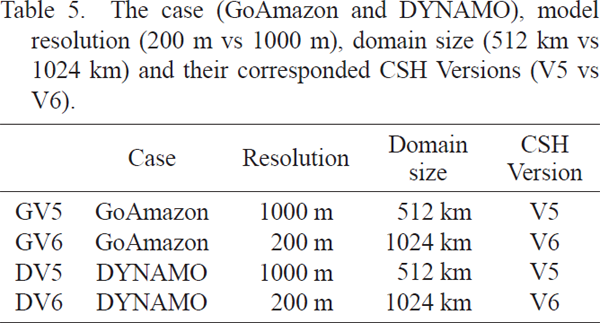
Figure 2 shows the time series of domain-averaged rain rates for the GoAmazon and DYNAMO cases both simulated using the GCE model and estimated from their respective sounding networks. The temporal variation of the GCE model-simulated rainfall is in very good agreement with the sounding estimates for both cases (especially for heavy rainfall events). The good agreement is caused by the fact that the GCE model is forced by the large-scale tendencies in temperature and water vapor computed from the sounding network. When the imposed large-scale advective forcing cools and moistens the environment, it increases the relative humidity; the model responds by producing clouds through condensation and deposition (release heat). The fallout of large precipitation particles produces the rainfall at the surface. Some precipitation particles evaporate before reaching the ground (absorbed heating or cooling). The stronger (weaker) the imposed advective forcing is, the more (less) cloud, precipitation, and surface rainfall is simulated (see Soong and Tao 1980). On the other hand, the km model will not produce cloud or rainfall when the imposed forcing heats and dries the atmosphere [e.g., around March 14 during GoAmazon (GV5 and GV6 simulations) and near and after November 30 during DYNAMO (DV5 and DV6 simulations)]. There is also good agreement in the GCE-simulated rainfall between the DV5 and DV6 simulations and between the GV5 and GV6 simulations (Fig. 2).

Fig. 2.

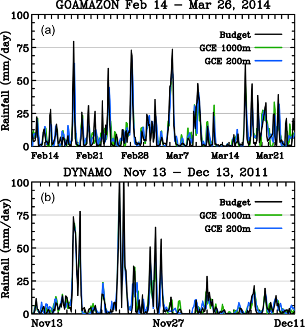
Time series of 2D GCE-simulated domainaverage surface rainfall using a 512 km horizontal domain at 1 km resolution (green) and a 1024 km horizontal domain at 200 m resolution (blue) versus surface rainfall derived from the corresponding sounding budget (black) for the (a) GoAmazon and (b) DYNAMO cases.

There is no direct observation for LH. However, a sounding network can be used to estimate the apparent heat source (or Q₁) as defined by Yanai et al. (1973). The GCE-simulated Q₁ can be validated with the sounding estimated Q₁. Figure 3 shows time series of domain-averaged total heating profiles simulated with the GCE model and Q₁ profiles derived from the sounding networks for both the GoAmazon and DYNAMO cases. Clearly, the model responds quite well to the imposed large-scale forcing for both cases. DYNAMO (oceanic case) has fewer but larger (longer lasting) events, whereas GoAmazon (continental case) has more numerous (shorter lasting) events. One notable difference in the DYNAMO case is that the GCE simulated less cooling between late November and early December. For the GoAmazon case, the GCE-simulated Q₁ also has less cooling in middle March as well as between active events. Another noted difference between the GCE modeled and sounding estimated Q₁ is that the simulated Q₁ does not show diurnal variation in the upper troposphere.

Fig. 3.

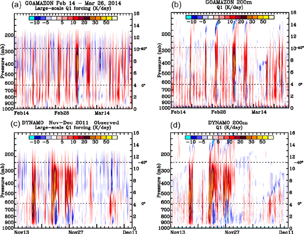
Time series of the domain-average apparent heat source (Q₁) derived from (a) the sounding network and (b) the GCE 200 m simulation for the GoAmazon case. (c) and (d) are the same as (a) and (b), respectively, except for the DYNAMO case.

Figure 4 shows multiday mean vertical profiles of Q₁ from the sounding estimates (40 days for GoAmazon and 31 days for DYNAMO) and the GCE simulations (GV5 and GV6, and DV5 and DV6, respectively). These profiles are the time averages of the profiles shown in Fig. 3. The higher resolution (GV6 and DV6) and lower resolution (GV5 and DV5) model-simulated Q₁ profiles are almost identical, and the simulated profiles are almost identical to the sounding estimated. The results indicate that the model resolution is not a major factor for the GCE-simulated Q₁ and total rainfall amount (see Table 6). However, the 200 m simulations are in slightly better agreement with the sounding estimated at midlevels (i.e., between 3 km and 4 km) in both cases.

Fig. 4.

Domain and time-mean Q₁ derived from the corresponding sounding budgets (black) versus simulated with the 2D GCE using a 512 km horizontal domain at 1 km resolution (green) and a 1024 km horizontal domain at 200 m resolution (blue) for the (a) GoAmazon and (b) DYNAMO cases.

The total domain-averaged rainfall amount and stratiform percentage from all four GCE experiments are shown in Table 6. The corresponding sounding estimated surface rainfall rates are 9.45 mm day⁻¹ and 8.23 mm day⁻¹ for GoAmazon and DYNAMO, respectively. Both GCE GoAmazon and DYNAMO-simulated total rainfall amounts are slightly overestimated (∼ 3 %) versus the sounding estimated. The results also indicate that there is only a very small difference in the total domain mean rainfall amount between the 200 m and 1000 m model simulations for both cases. The results from Fig. 2 and Table 6 indicate that the model resolution does not have much impact on the GCE-simulated rainfall. The good agreement in surface rainfall and Q₁ between the GCE simulations and the sounding estimates is the main reason for using the GCE (or other CRMs with the same imposed large-scale advective forcing approach) to produce LH for the CSH (and SLH) algorithm.

The stratiform percentages using different model resolution as well as different convective-stratiform separation methods are shown in Table 6. The total mean rainfall is about 15 % more in the GoAmazon case than in the DYNAMO case. This is because the large-scale advective forcing is larger in GoAmazon. Interestingly, the stratiform percentage is not sensitive to the convective-stratiform separation methods for CSH V6 (i.e., only a 0.3 % difference in GoAmazon and 0.6 % in DYNAMO). For CSH V5, the stratiform percentage is higher using the GCE method for both the GoAmazon and DYNAMO cases. There are 7.2 % and 8.8 % more stratiform rain with the GCE separation than the 2A23-type method in GV5 and DV5, respectively. The results indicate that the stratiform rainfall amount (percentage) is more sensitive to the convective-stratiform separation method for CSH V5.

The convective-stratiform separation methods are different for CSH V5 and V6, the GCE and 2A23-type methods, respectively. For the GoAmazon case, GV5 has a 4.7 % greater stratiform percentage than GV6. The stratiform percentage is 38 % using the 2A23-type method in DV6 and 41 % using the GCE method in DV5, so there is a 3 % higher stratiform percentage in DV5 than in DV6.

Overall, the simulated Q₁ (Fig. 4) and surface rainfall (Table 6) between GV5 and GV6 are very similar as they are between DV5 and DV6. The model-simulated stratiform percentage is also not sensitive to the model resolution when using the same convective-stratiform separation method. The Q₁ in the convective and stratiform regions is examined using the CSH V6 runs (200 m GCE model resolution). Figures 5 and 6 show the time series of domain-average GCE-simulated Q₁ in the convective and stratiform regions using the two different convective-stratiform separation methods (2A23-type and GCE) for GoAmazon and DYNAMO, respectively. Overall, the temporal variation of the Q₁ profiles in the convective and stratiform regions is similar using the different convective-stratiform separation methods.

Fig. 5.

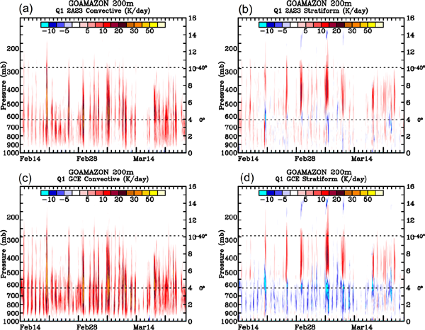
Time series of domain-average GCE-simulated Q₁ in the (a) convective and (b) stratiform regions using a 2A23-type convective-stratiform separation. (c) and (d) are same as (a) and (b), respectively, except that the convective-stratiform separation is based on the GCE method.

Fig. 6.

Same as Fig. 5, except for the DYNAMO case.

For the GoAmazon case, Q₁ profiles in the convective region show the classic vertical distribution of heating from the low to upper troposphere. Convective Q₁ is stronger in the GCE's convective-stratiform separation than that of the 2A23-type method. Q₁ profiles in the stratiform region also exhibit the classic vertical distribution of heating aloft and cooling beneath the freezing level. However, cooling is much stronger in the GCE's convective-stratiform separation than in the 2A23-type method. In addition, there is frequent low-level heating in the stratiform region (see Fig. 5b) using the 2A23-type method. Heating is mainly associated with very light rainfall events. However, the stratiform Q₁ profiles from the GCE method have almost all cooling below the freezing level (Fig. 5d). This is another major difference using the different convective-stratiform separation methods.

For the DYNAMO case, convective heating is much stronger using the GCE's convective-stratiform separation method than the 2A23-type method (Figs. 6a, c). Cooling is also much stronger with the GCE separation (Figs. 6b, d). Low-level heating also appears in the stratiform region using the 2A23-type method. The difference between the GoAmazon and DYNAMO cases is that convective heating and stratiform cooling are stronger in DYNAMO (see Fig. 7). First, it is due to the difference in the advective forcing imposed into the GCE model simulations (Fig. 3). There are two major (and large) organized convective events associated with the MJO with strong heating aloft and cooling beneath (November 22–23 and November 25–26) for the DYNAMO case. Their simulated Q₁ in the convective and stratiform region mainly is the response to the imposed forcing.

Fig. 7.

Same as Fig. 4, except (a) for the convective regions from the two 2D GCE simulations using the 2A23-type separation applied at the model resolutions and 4 km and the GCE separation applied at the model resolutions for the GoAmazon case. (b) is the same as (a), except for the stratiform regions, and (c) and (d) are the same as (a) and (b), respectively, except for the DYNAMO case. (b) and (d) also show the 2A23-type separation applied at 4 km for deep stratiform regions only (Str5; echo tops > 5 km).

Figure 7 shows the multiday mean vertical profiles of Q₁ from the convective and stratiform regions for the two different convective-stratiform separation methods for both the GoAmazon and DYNAMO cases. These profiles include the time averages of the profiles shown in Figs. 5 and 6. In addition, the results from the coarser model resolution (1000 m), the 2A23-type separation applied at the model resolution, and the 2A23-type separation applied at 4 km resolution (V6 LUTs) for deep stratiform only (Str5, echo tops > 5 km) are shown for comparison. Both the Go Amazon and DYNAMO cases have heating in the convective region using the two different separation methods. However, heating is stronger using the GCE method than the 2A23-type method for both cases. Applying the 2A23-type method at the model resolution also results in stronger heating but not as strong as that for the GCE method. Both cases show heating aloft in the stratiform region. However, low-level (below 4 km) cooling is only shown in the GCE method or the 2A23-method when applied at the model resolution for both the GoAmazon and DYNAMO cases. There is no mean low-level cooling in the stratiform region in the 2A23-type method when applied at 4 km (V6 LUT) resolution. This is due to areas of weak low-level heating that are classified as shallow stratiform (e.g., weak or dissipating congestus-type clouds) by the separation method being averaged with the weak cooling of the deep stratiform profiles in the model data. If the 2A23-type stratiform areas derived at 4 km resolution are conditioned on deep stratiform only (echo tops > 5 km), classic stratiform heating over cooling profiles emerges.

The Q₁ profiles in the convective and stratiform regions are quite similar for the two different model resolutions (1000 m and 200 m). This is consistent with the surface rainfall amounts (Fig. 2 and Table 6) and total Q₁ (Fig. 4). This result indicates that the model resolution does not have a major impact on the time- and domain-averaged Q₁ and LH due to the same imposed large-scale advective forcing. However, it still could be important at smaller scales/regions.

Figure 8 shows the CSH V5 and V6 LH LUTs for convective (down increasing echoes only) echo-top height bins of 0–2, 4–6, and > 8 km and stratiform bins of 0–2 km downward increasing and > 8 km for both downward increasing and downward decreasing echoes in the lowest 2 km. Only the oceanic LUTs are shown for comparison. The V5 LUTs are for the most convective and most stratiform bins for the gridded product (Lang and Tao 2018), which was the primary product for V5, and the V6 LUTs are for the pixel product, which is the primary product for V6. Note that the LUTs shown in Lang and Tao (2018) where for 19 levels. The plots shown in Fig. 8 use 80 levels, which is what is used for the actual retrievals for both V5 and V6.

Fig. 8.

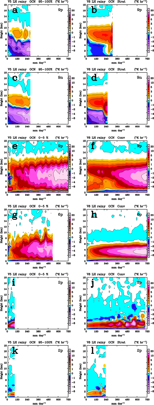
Comparison of CSH V5 and V6 LH LUTs for stratiform echo-top height bins of > 8 km for both downward increasing (a, b) and downward decreasing (c, d) echoes in the lowest 2 km as well as convective (downward increasing echoes only) echo-top height bins of > 8 km (e, f), 4–6 km (g, h), and 0–2 km (i, j). Shallow stratiform (downward increasing echoes) LUTs for echo-top heights of 0–2 km are shown in (k) and (l). The V5 LUTs (a, c, e, g, i, k) are for the most convective and most stratiform bins for the gridded product, which was the primary product for V5, and the V6 LUTs (b, d, f, h, j, l) are for the pixel product, which is the primary product for V6.

Overall, the basic heating structures are similar between V5 and V6. For example, there is heating aloft and cooling below in the stratiform region, and almost all heating in the convective region. However, there are some notable differences. The heating in the stratiform region is much stronger in V6 than in V5, but low-level cooling in V6 is weaker than that in V5. There is another difference in the stratiform region for high rainfall rates (i.e., > 240 mm day⁻¹), where there is low-level heating in the V6 LUT but not in the V5 LUT. For the convective region, the maximum heating is quite similar in both the V5 and V6 LUTs, but the level of maximum heating is lower in V6 than its V5 counterpart. Midlevel heating is also stronger in V5 than in V6 (Figs. 8e, f). Another difference is that the vertical extent of heating is also lower for V6 than for V5 (2 km height difference), except for the lowest level LUT (2p) shown in Figs. 8i and 8j. Shallow stratiform LUTs (Figs. 8k, l) are similar to shallow convective, except for having much weaker heating, and are indicative of weak or dissipating congestustype clouds.

Lang et al. (2003) examined six different convective- stratiform separation methods, and their results showed that the GCE method had a higher stratiform rainfall percentage than the Steiner method for two squall line cases (Table 3 in Lang et al. 2003). Their results also showed that LH retrieval can be sensitive to the use of separation technique mainly as a result of differences in the stratiform region.

4. CSH V6-retrieved LH

4.1 Vertical profiles of CSH-derived LH

The LH profiles for the total, convective, and stratiform regions for six different geographic locations are shown in Fig. 9. Because different convective-stratiform separation methods are applied in the CSH and SLH LUTs, both the CSH and SLH algorithm-retrieved LH are shown for comparison. Table 7 shows the surface rain rate (mm day⁻¹) and stratiform percentage (%) for these six regions. For the South China Sea Monsoon Experiment (SCSMEX) region, the derived surface precipitation rate is 2.59 mm day⁻¹ with 68.83 % stratiform; for the Global Atmospheric Research Program's Atlantic Tropical Experiment (GATE) region, the surface precipitation rate is 9.36 mm day⁻¹ with 40.06 % stratiform; for the DYNAMO region, it is 5.47 mm day⁻¹ with 36.56 % stratiform; for the Tropical Ocean Global Atmosphere – Coupled Ocean Atmosphere Response Experiment (TOGA COARE) region, it is 10.65 mm day⁻¹ with 42.78 % stratiform; for the GoAmazon region, it is 3.71 mm day⁻¹ with 35.18 % stratiform; and for the SW of Australia region, it is 3.26 mm day⁻¹ with 81.26 % stratiform. The stratiform percentage is based on the satellite separation method.

Fig. 9.

CSH- and SLH-retrieved mean total, convective, and stratiform vertical LH profiles for July, August, and September of 2014 for six different geographic regions: (a) TOGA COARE, (b) GATE, (c) DYNAMO, (d) GoAmazon, (e) SCSMEX, and (f) SW of Australia during SH winter. Black, red, and blue lines show the total, convective, and stratiform areas, respectively. Solid lines are for CSH, and dashed lines are for SLH.

There are several differences between the CSH- and SLH-derived total LH profiles over the five tropical/warm season regions (i.e., TOGA COARE, GATE, DYNAMO, GoAmazon, and SCSMEX). The CSHderived LH profiles are larger than their corresponding SLH profiles for all five regions. Also, the SLH-derived LH profiles show three local heating maxima, namely, at 2, 4, and 7 km, for the TOGA COARE, GATE, and DYNAMO regions. The CSH-derived LH profiles have two heating maxima, that is, one at the 2.5–3 km level and one at 6 km, for these three regions. On the other hand, CSH- and SLH-derived LH profiles both have one main heating maximum, around 6 km for SCSMEX and GoAmazon and around 3.5 km for the region SW of Australia.

Both the CSH- and SLH-retrieved LH profiles also have characteristics of convective and stratiform LH as shown by Tao et al. (2001). There are heating in the convective region and heating aloft but cooling beneath in the stratiform region. There is also small low-level (near surface) cooling in the convective region in all cases for both the CSH- and SLH-derived profiles. The regional CSH-retrieved LH profiles display these signature profiles even though the mean model stratiform profiles using the 2A23 method at 4 km resolution shown in Figs. 7b and 7d are not due to the 4 km averaging and the mixing of deep and shallow stratiform in the model mean profiles.

The geographic regions with a higher mean surface precipitation rate (i.e., TOGA COARE and GATE) have larger convective heating. The convective heating in the SCSMEX and GoAmazon regions, which have lower mean surface rain rates, is weaker versus that in the GATE and TOGA COARE regions. Convective heating at middle and upper levels is stronger in the CSH-derived profiles than in the SLH for these five regions. However, the heating aloft in the stratiform region is stronger for SLH in all cases. The level of maximum convective heating is higher in all regions in the CSH profiles versus the SLH. In terms of stratiform cooling in the lower troposphere, both CSH and SLH cooling are of similar magnitude and shape. However, mean cooling starts up to ∼ 1 km higher (near 5 km for TOGA COARE, GATE, DYNAMO, and GoAmazon and 4 km for SCSMEX) for SLH versus CSH. For the cold case (SW of Australia region), there is greater similarity between the CSH- and SLH-derived convective and stratiform LH profiles than the other five tropical regions. Both CSH- and SLH-derived convective heating is much smaller than their stratiform counterparts, and low-level cooling only occurs from the surface to the 250 m level.

Figure 10 shows zonal cross sections of the three month mean LH profiles for the old (V5) and new (V6) versions of the CSH algorithm. The overall shapes are quite similar. Heating is stronger in the tropics and peaks at a higher level (∼ 6 km) than in middle and higher latitudes (below 5 km) in both versions. Both also exhibit low-level heating (below ∼ 2.5 km) in the tropics. However, heating at middle levels (∼ 2 km to 5 km) is reduced in the tropics in V6 compared to V5 and is the main reason for the reduced bias in the zonal mean vertically integrated CSH heating versus the Combined algorithm surface rain as shown in Fig. 11a. In the net, there is weak cooling at the lowest levels in both the tropics and extratropics for both versions, which is slightly deeper in the Northern Hemisphere in V6.

Fig. 10.

Latitude–height cross sections of three month mean zonal LH from the (a) new (V6) and (b) old (V5) CSH algorithm. The two horizonal lines indicate 5 km and 7 km altitude.

Fig. 11.

Zonal mean vertically integrated CSH-retrieved diabatic heating versus surface rainfall rate (mm day⁻¹) from the GPM Combined Algorithm for the three month period from July 1 to September 30, 2014. (a) is total, (b) is over the ocean only, and (c) is for land only. Green line is from V6, and blue line is from V5.

4.2 Relationship between vertically integrated latent heating and surface precipitation

In a diagnostic study (e.g., Yanai et al. 1973), the apparent heat source (Q₁) of a large-scale system is defined by averaging horizontally the thermodynamic equation (θ, potential temperature) as follows:   

Note that Q₁ can be calculated either from observations or from grid values in a large- or regional-scale prediction model. π = (p/p₀₀)^R/c_p is nondimensional pressure (where p and p₀₀ are dimensional and reference pressures, respectively, with p₀₀ taken as 1000 hPa). Q₁ is directly related to the contribution of cloud effects, which can be explicitly estimated from the GCE model (Soong and Tao 1980; Tao and Soong 1986; Tao and Simpson 1989):   

where overbars denote horizontal averages (or model horizontal domain averages) and primes indicate deviations from the large-scale environment due to smaller scale cloud processes. The variable ρ is density, c_p is the specific heat of dry air at constant pressure, R is the gas constant for dry air, and Q_R is the radiative heating rate. The variables L_v, L_f, and L_s are the latent heats of condensation, fusion, and sublimation, respectively, and the variables c, e, f, m, d, and s are the condensation of cloud droplets; evaporation of cloud droplets and raindrops; freezing of water droplets and raindrops; melting of ice crystals, snowflakes, graupel, and hail; deposition of ice crystals and snowflakes; and sublimation of all ice hydrometeors, respectively. Note that the latent heat of fusion is one order smaller than the latent heat of condensation and sublimation. 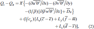The term is the LH due to microphysical phase changes, and the first three terms on the right-hand side (RHS) of Eq. (2) are the two horizontal divergence and vertical heat flux (transport), respectively. D_θ is the turbulence term, and its value is smaller than the other terms. The horizontal divergence terms are usually neglected when Eq. (2) is spatially averaged over an area suitable for diagnostic analysis. The domain-averaged horizontal divergence term is zero in the GCE model simulations because cyclic lateral boundary conditions are used.

There is a relationship between column-integrated apparent heating, radiation effects, the net surface precipitation, and the net surface heat fluxes as shown in the following equation (see Yanai et al. 1973):   

where P_o is the surface precipitation rate, S_o is the surface heat flux, g is gravity, and L_v is the latent heat of condensation. Lx and Ly are the horizontal lengths of the x- and y-directions, respectively, and Ptop and Psfc are the cloud top and surface, respectively. In order to derive Eq. (1), Yanai et al. (1973) stated that “we consider an ensemble of cumulus clouds, which is embedded in a tropical large-scale motion system, then we imagine a horizontal area that is large enough to contain the ensemble of clouds, but small enough to be regarded as a fraction of the large-scale system”.

Replacing the left-hand side of Eq. (1) with the RHS of Eq. (2) and vertically integrating the RHS of Eq. (2) give a relationship between LH and the surface rainfall and sensible heat fluxes (i.e., the RHS of Eq. 1). The retrieved LH can therefore, be vertically integrated to produce an “equivalent surface rain rate”, which can then be compared against the GPM Combined-derived (input) surface rain rate to check its performance (and biases).

In the tropical-warm season GCE model simulations, surface heat fluxes are calculated using the TOGA COARE flux algorithm (Wang et al. 1996, 2003) for all ocean cases, except for DYNAMO, in which they are prescribed. Over land, the TOGA COARE flux algorithm is used for the two Department of Energy (DOE) Atmospheric Radiation Measurement cases, but surface fluxes are prescribed for the Midlatitude Continental Convective Clouds Experiment (MC3E) and GoAmazon cases. For the TOGA COARE flux algorithm, each surface model grid point has its own fluxes. The prescribed fluxes vary in time but are applied horizontally uniform over all surface grid points.

4.3 CSH-derived zonal mean vertically integrated Q₁–Q_R

Three-month (July, August, and September 2014) zonal mean vertically integrated 3GCSH-retrieved equivalent surface rain rates (Q₁–Q_R) are shown in Fig. 11a. This particular period was selected because of the overlap between TRMM and GPM. The GPM Combined algorithm-derived mean surface rain rates are also shown for comparison. The equivalent and Combined-derived surface rain rates are in excellent agreement in the Inter Tropical Convergence Zone (ITCZ) region/deep tropics (5–17°N). They are also in very good agreement over the high latitudes in the Northern Hemisphere (∼ 30°N to 65°N) as well as the region from ∼ 20°S to 40°S in the Southern Hemisphere. However, the equivalent surface rain rates are higher than the Combined surface rain rates in the subtropics (the maximum difference is around 20°N and 15°S in the Northern and Southern Hemispheres, respectively). Note that eddy fluxes are not included in the V6 cold season LUTs generated from NU-WRF model simulations. Overall, the eddy fluxes are quite small in the warm season cases.

The equivalent and Combined surface rain rates over the ocean only and land only are shown in Figs. 11b and 11c, respectively. Note that the area covered by the ocean, especially in the tropics and subtropics, is much larger than the area covered by land. In the TRMM domain, the good agreement between the equivalent and Combined-derived surface rain rates as shown in Fig. 11a is mainly from the ocean region (Fig. 11b). In general, equivalent surface rain rates are larger than the Combined surface rain rates over land (Fig. 11c). The difference is quite large in the deep tropics (5°S to 5°N) and subtropics in the Northern Hemisphere. Outside of the TRMM domain, there is good agreement between the equivalent and Combined surface rain rates over land in the Northern Hemisphere. This is the reason for the good agreement between the equivalent and Combined-derived total surface rain rates there (Fig. 11a). The equivalent surface rain rate is higher (lower) than the Combined derived in the Southern (Northern) Hemisphere. Because the ocean has a smaller area coverage in the Northern Hemisphere, its contribution to the total surface rain rate is lower than its land counterpart. On the other hand, the ocean covers a larger area in the Southern Hemisphere, so it has a larger contribution to the total surface rain rate. That is why both the total surface rain rate and its ocean component are larger (higher) than those from the Combined algorithm (Figs. 11a, b). These differences and similarities between the equivalent and Combined-derived surface rain rates can provide guidance for improving the CSH algorithm in the future, as well as potential applications for users.

Figure 11 also shows the same three-month (July, August, and September 2014) zonal mean vertically integrated retrieved equivalent surface rain rates for the previous V5 algorithm. Although the biases are comparable over the ocean (though V6 still shows notable improvement especially in the Southern Hemisphere), V5 clearly has much larger positive biases than V6 over land. The net result is that V6 has significantly reduced biases over nearly every latitude compared to V5 and is therefore, in much better overall heat balance.

Figure 12a shows the three-month (July, August, and September 2014) CSH vertically integrated Q₁–Q_R (equivalent surface rain rate). The GPM Combined algorithm-derived surface rain rate is also shown in Fig. 12b for comparison. The horizontal distribution (or pattern) between the equivalent and Combined-derived surface rain rates is quite similar. For example, both show high rainfall rates over the ITCZ, the South Pacific Convergence Zone (SPCZ), and the midlatitude storm track (along the east coast of China and North America), and at mid-to-high latitudes (30–50°S) in the Southern Hemisphere. In addition, light rain rates or no surface rainfall occurs over the west coast of both the American and African continents, and Australia.

Fig. 12.

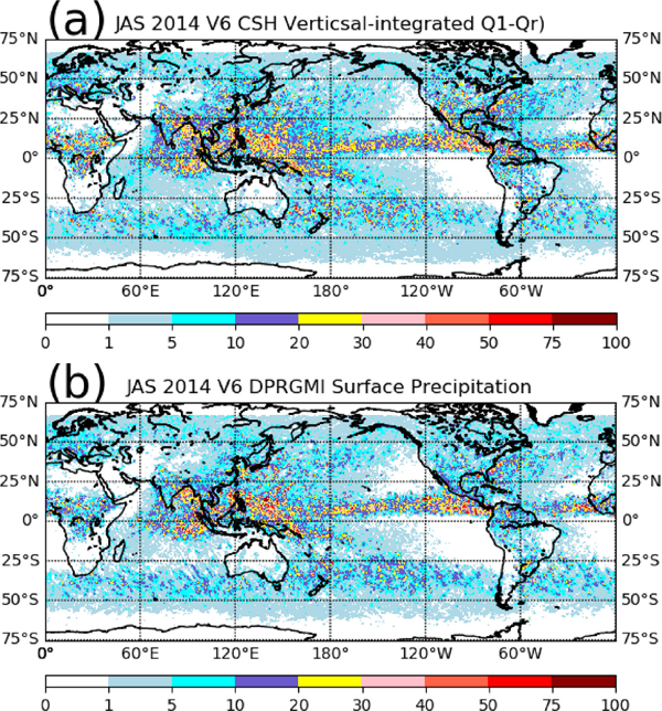
Three-month mean (a) CSH vertically integrated Q₁–Q_R (equivalent surface rain rate) and (b) Combined algorithm surface rain rate (mm day⁻¹). Results are for July, August, and September 2014 at 0.25° × 0.25° resolution.

The net difference between the CSH equivalent (3GCSH, 0.25° × 0.25°) and the GPM Combined surface rain rates over the same three-month period from July 1 to September 30, 2014 is shown in Fig. 13a. Clearly, the differences between the equivalent and Combined-derived rainfall rates are larger over the regions with high rainfall rates (Fig. 11). Over land, the equivalent surface rain rate is larger than the Combined derived over central Africa, the Indian subcontinent, Southeast Asia, and America (including Central America, the Southwest US, and northern South America). These estimates are also evident in Fig. 11c (from 10°S to 25°N). Over the ocean, the equivalent surface rain rate is larger than the Combined derived over the Pacific Ocean (especially, the SPCZ, the Central and West Pacific). Overall, the difference is larger in terms of intensity (rainfall rate) as well as the areal coverage over land than that over the ocean.

Fig. 13.

The difference between the CSH equivalent and Combined surface rain rates (mm day⁻¹). (a) is for 0.25° × 0.25°, (b) is for 0.5° × 0.5°, and (c) is 1.0° × 1.0° resolution.

Yanai et al. (1973) stated that the area “is large enough to contain the ensemble of clouds, but small enough to be regarded as a fraction of the large-scale system” for Eq. (3). Figures 13b and 13c show the differences averaged into 0.5° × 0.5° and 1.0° × 1.0°, respectively. The differences between the equivalent and Combined-derived surface rain rates are still present in both Figs. 13b and 13c. However, the local differences are smaller for the larger area averages compared to the smaller area averages. Note that the averages are a simple arithmetic area averaged from high resolution (i.e., 0.5° × 0.5° is from 0.25° × 0.25°, and 1.0° × 1.0° is from 0.5° × 0.5°). Note that the bias is the same in these figures (Figs. 13a, b, c) because this arithmetic average is used. The results suggest that users need to consider averaging the CSH standard product, 3GCSH (0.25° × 0.25°), to coarser resolution for their specific applications.

Figures 14a and 14b show the mean surface rainfall from the Combined algorithm for the three-month period of July, August, and September 2014 for both TRMM and GPM. The mean rainfall is from the 0.25° × 0.25° standard gridded product. Note that the TRMM domain is about 37°S to 37°N, and the GPM domain is about 67°S to 67°N. All observed tropical major rainfall regimes, such as the ITCZ, the SPCZ, the Maritime Continent, and midlatitude storm tracks, are captured in both the TRMM and GPM Combined algorithm-derived surface rainfall. However, the mean rain rates in the ITCZ region (Central Pacific, Atlantic, and Indian ocean) as well as the subtropical oceans are higher for GPM, which is consistent with GPM's ability to detect lighter rain rates (Hamada and Takayabu 2016). Rainfall rates over land are also higher for GPM. Table 8 shows the mean surface rainfall rates for TRMM and GPM. Within the TRMM domain, GPM has a slightly higher mean rainfall rate than TRMM (2.91 mm day⁻¹ vs. 2.85 mm day⁻¹). The higher surface rain rates occur over both land and ocean. However, the difference in the surface rain rate is higher over land (2.49 mm day⁻¹ vs. 2.37 mm day⁻¹) than over the ocean (3.09 mm day⁻¹ vs. 3.05 mm day⁻¹).

Fig. 14.

Mean surface precipitation rate (mm day⁻¹) from the Combined algorithm for the three-month period July, August, and September 2014 for (a) TRMM and (b) GPM, and the stratiform rain percentage for (c) TRMM and (d) GPM at 0.25° × 0.25° resolution. Note that TRMM only covers the tropics and subtropics and GPM extends to higher latitudes.

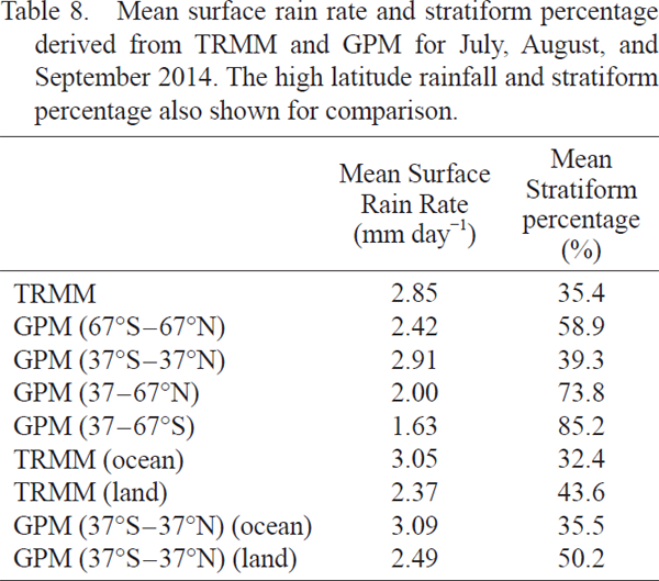
The corresponding surface rainfall stratiform percentage for both TRMM and GPM is shown in Figs. 14c and 14d, respectively. High stratiform percentages (40–50 %) are associated with regions over the ITCZ, the SPCZ, and the Maritime Continent, whereas low stratiform percentages (∼ 5–10 %) are over the coast of South America and the Atlantic and Indian Oceans (between the equator and 25°S). These features are quite similar between TRMM and GPM in the tropics. Over the TRMM domain, the mean stratiform percentages are 35.0 % and 39.3 %, respectively, for TRMM and GPM (see Table 8). The higher stratiform percentage for GPM occurs over both land (50.2 % vs. 43.6 %) and ocean (35.5 % vs. 32.4 %). The stratiform percentage and the total surface rainfall amount are the two major factors that determine the vertical distribution of CSH-retrieved LH (Tao et al. 1993). Specifically, a higher stratiform rain percentage produces a higher altitude of maximum LH. A higher surface rainfall amount has stronger LH. The difference in the mean rainfall rate is 0.6 mm day⁻¹ (or 2 %) between TRMM and GPM. The difference in the stratiform rain is only about 3.9 %. Consequently, these differences may not have a major impact on the mean vertical distribution of LH (Tao et al. 1993).

Outside the TRMM domain, there are very high stratiform percentages (∼ 70 %) at higher latitudes (Fig. 14d). The high stratiform feature is associated with light rainfall rates (Fig. 14b) and midlatitude precipitation systems (Yokoyama et al. 2017). For the Northern Hemisphere, its mean rainfall rate is higher than its counterpart in the Southern Hemisphere, but its mean stratiform rain percentage is less than its counterpart in the Southern Hemisphere (Table 8). In addition, the mean rainfall area is much larger in the Southern Hemisphere than in the Northern Hemisphere (Fig. 14b). This suggests that the mean rainfall rate is weak (light rainfall) in the Southern Hemisphere. Note that July, August, and September are during summer (winter) in the Northern Hemisphere (Southern Hemisphere). The seasonal difference could be one of the main reasons for the difference in mean surface rain rates and its stratiform component.

Figure 15 shows the three-month zonal mean CSH-retrieved equivalent surface rain rates for TRMM and GPM. The surface rain rates derived from the TRMM and GPM Combined algorithm are also shown in Fig. 15 for comparison. The CSH equivalent surface rain rates for TRMM and GPM are in very good agreement with each other. The TRMM and GPM Combined-derived surface rain rates are also in excellent agreement with each other. Note that the same equivalent and Combined-derived zonal mean surface rain rates for GPM were already shown and discussed in Fig. 11. The equivalent surface rain rates are in slightly better agreement with the Combined derived for TRMM than GPM in the Southern Hemisphere (20°S to the equator). The same good agreement in the deep tropics (ITCZ region, from 5°S to 15°N) is also shown in the CSH equivalent surface rainfall for TRMM. However, local differences still occur with the surface rain rate for TRMM (similar to Fig. 13).

Fig. 15.

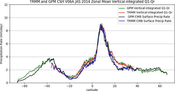
Same as Fig. 11a, except for TRMM and GPM. The black and blue lines are the mean surface rain rate (mm day⁻¹) from the Combined algorithm for GPM and TRMM, respectively. The green and red lines are the CSH-retrieved vertically integrated Q₁–Q_R from TRMM and GPM, respectively.

In addition to the Northern Hemisphere's warm season, the CSH-retrieved equivalent and GPM Combined-derived zonal mean surface rainfall rates for the Northern Hemisphere's cold season (November and December 2014 and January 2015) are shown in Fig. 16a. Overall, the CSH-retrieved equivalent surface rain rates are in very good agreement with the GPM derived for the Northern Hemisphere, especially in the deep tropics – ITCZ region (0–15°N). This excellent agreement is consistent with the results from the warm season in the Northern Hemisphere (Fig. 11a). The results also show that the equivalent surface rain rates are in better agreement for the cold season (November and December 2014 and January 2015 in the Northern Hemisphere and July, August, and September 2014 in the Southern Hemisphere) than the warm season in both hemispheres (see Figs. 11, 16).

Fig. 16.

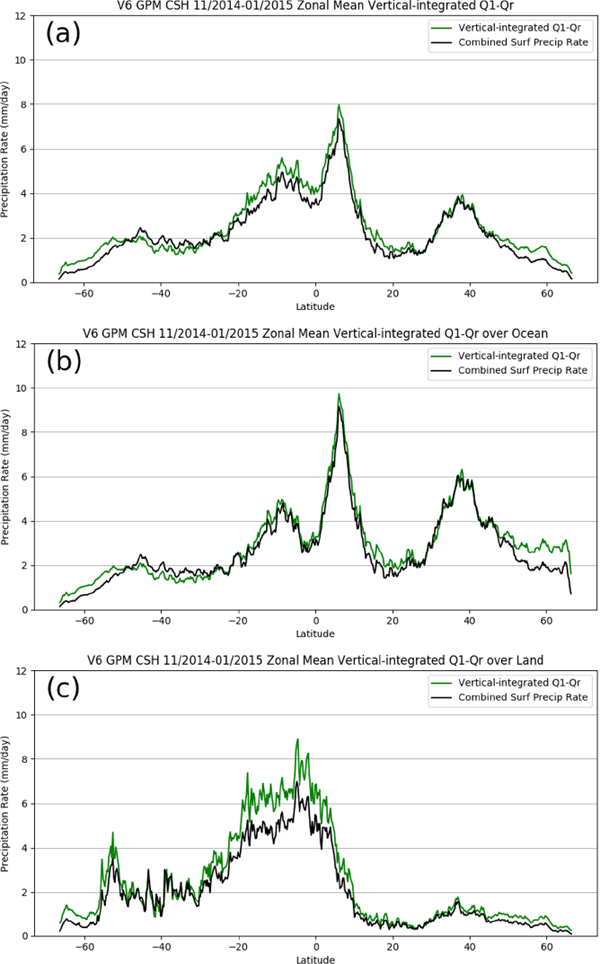
Same as Fig. 11, except for the threemonth period from November 1, 2014 to January 31, 2015.

The corresponding surface rain rates from ocean and land regions are shown in Figs. 16b and 16c, respectively. The high CSH-retrieved equivalent surface rain rates in the deep tropics – ITCZ region are mainly from the ocean region and are in excellent agreement with the Combined derived. This result is consistent with that from the Northern Hemisphere's warm season (Fig. 10b). The CSH equivalent surface rain rates are in better agreement with the Combined derived over the ocean than over land. Equivalent surface rain rates from 20°S to 5°N over land are higher compared to the Combined derived. This is also consistent with the Northern Hemisphere's warm season (Fig. 11c).

Figure 17 shows the one-to-one correlation between CSH-retrieved equivalent and GPM-derived surface rain rates for the Northern (Southern) Hemisphere's warm (cold) season. The surface rain rate is the monthly gridded data (level 3). The results indicate that there is more scatter for light rainfall rates. Both Northern Hemisphere's three-month cold and warm seasons show very similar correlations between the CSH equivalent and Combined-derived surface rainfall rates with a quite high correlation coefficient of 0.99. However, the CSH-retrieved equivalent surface rain has more light rain rates than the Combined derived. In addition, it has fewer large rain rates than the Combined derived.

Fig. 17.

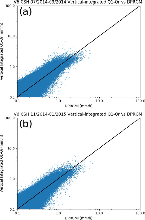
Scatterplots showing the co-relations between CSH equivalent and GPM-derived surface rainfall rate. (a) is for July, August, and September 2014 and (b) is for November and December 2014 and January 2015.

5. Summary and future work

Two different numerical models, namely, the GCE and NU-WRF, have been used to generate CSH LH LUTs. The GCE-generated LUT is for the tropical-warm season, and the NU-WRF generated is for the high latitude – cold season. For the tropical-warm season, the GCE model-simulated LH is from high-resolution (200 m) simulations, and the convective-stratiform separation method is more consistent with that for the GPM DPR. These are the two major differences between the current V6 CSH and the previous V5 CSH. Long-term GCE model simulations for one continental (GoAmazon) and one oceanic (DYNAMO) case are conducted to examine these differences (convective and stratiform separation method and model resolution). Sounding network estimated Q₁ and surface rain rate are used for comparison. For the high latitude – cold season, the NU-WRF-simulated LH LUTs do not use convective-stratiform separation, but simulated LH structures still have convective-like and stratiform-like structures (Tao et al. 2019).

Officially, the CSH algorithm is used with precipitation products from the GPM DPR-GMI and TRMM PR-TMI Combined algorithm (i.e., surface precipitation rates, composite radar reflectivity, freezing level height, and echo-top height) as input (see Fig. 1). Because there is no direct measurement of LH, comparisons between the CSH vertically integrated heating equivalent surface rainfall rates and the Combined algorithm-derived surface rain rates are used to examine CSH performance. The major highlights are as follows:

• ・The GCE-simulated Q₁ profiles and the temporal variation of the surface rain are in very good agreement with those from sounding estimates for both the GoAmazon and DYNAMO cases.
• ・The GCE-simulated total Q₁ profile and its convective and stratiform component are almost identical for two different model resolutions (1000 m and 200 m) using the same convective-stratiform separation method.
• ・The GCE-simulated vertical profile of Q₁ in the convective and stratiform region is sensitive to the convective-stratiform separation method. Its simulated Q₁ shows heating from the low to upper levels in the convective region for both separation methods. Using the GCE separation method, the GCE-simulated Q₁ stratiform profiles show a classic structure, heating aloft and cooling beneath the melting level. Using the 2A23-type method, however, there is no (or very small) low-level cooling in the stratiform region.
• ・Mean CSH and SLH-retrieved LH profiles for five different regions in the tropics and subtropics (TOGA COARE, GATE, DYNAMO, GoAmazon, and SCSMEX) show heating in the convective region and heating aloft but cooling beneath in the stratiform region. These CSH and SLH-retrieved LH profiles display the classical heating profiles shown in Tao et al. (2000). This differs from the mean stratiform profiles extracted from the full GCE simulation data for GoAmazon and DYNAMO using the 2A23-type separation at 4 km resolution, which show little cooling or even warming below the freezing level, due to the inclusion of shallow stratiform in the model, some of which falls below the detection limit of the satellite.
• ・The CSH three-month and zonal mean equivalent and Combined-derived surface rain rates are in excellent agreement in the ITCZ region/deep tropics (5–17°N in the Northern Hemisphere warm season and 0–15°N in the Northern Hemisphere cold season). These agreements are mainly from the ocean region.
• The CSH three-month and zonal mean equivalent surface rain rates are larger than the Combined surface rain rates over land and in the deep tropics and subtropics in both the Northern Hemisphere warm and cold seasons.
• ・The CSH three-month mean equivalent surface rainfall and TRMM and GPM Combined-derived surface rainfall distributions capture many well-known weather features, such as the ITCZ, SPCZ, the Maritime Continent, and midlatitude storm tracks during the Northern Hemisphere warm season.
• The CSH three-month and zonal mean equivalent surface rain rates are in very good agreement using TRMM and GPM Combined-derived surface rain rates and precipitation properties. This good agreement could be caused by the fact that there is also a good agreement in surface rain rates derived by the TRMM and GPM Combined algorithm.
• ・The CSH three-month mean equivalent surface rainfall distribution has differences with the Combined-derived rainfall rates for both ocean and land regions. The difference is larger in terms of intensity (rainfall rate) as well as the areal coverage over land than that over the ocean. However, all of these differences can be reduced locally with arithmetic horizontal averaging (i.e., 3GCSH's 0.25° to coarser resolution, 0.5° or 1.0°) depending on specific applications.
• ・The CSH mean equivalent surface rainfall has more light and less large rainfall rates compared to the Combined derived even though there is a high correlation between the CSH mean equivalent and Combined derived.

It is expected that all PMM rainfall/snowfall and LH V7 retrieval algorithms will be released in late 2021/early 2022. The CSH algorithm LUTs will continue to be improved using 3D GCE model simulations for the tropical-warm season and additional NU-WRF simulations of synoptic cold season systems. For V7, radiative profiles and surface heat fluxes from NU-WRF will be added to the high latitude cold season.

The heating structure using the GCE method is more similar to the classic heating profile than that of the 2A23-type method (i.e., Houze 1982; Johnson 1984). Positive heating via condensation and deposition (and freezing) dominates throughout the column in the convective region. In the stratiform region, heating occurs above the melting level through deposition whereas cooling mainly from evaporation prevails beneath the melting level. However, the GCE method requires information on the vertical velocity as well as cloud properties to separate the convective and stratiform regions. This information is not directly available from TRMM and GPM nor other satellite missions. However, the future NASA satellite Aerosol, Cloud, Convection and Precipitation mission is planned to measure the vertical velocity and cloud/precipitation properties. The GCE convective-stratiform separation method could be utilized for this future satellite mission.

Surface heat fluxes could play a major role in the balance with equivalent surface rain rates as shown in Eq. (3). The large difference between the CSH-retrieved equivalent and Combined-derived surface rain rates over land might be caused by the land surface heat fluxes (these are mainly by the GCE model simulated or specified in the CSH V6). Both the CSH and SLH algorithm teams plan to examine the global energy balance between LH, precipitation, and surface heat fluxes based on physical understanding (via comparisons with global reanalysis and/or different precipitation features).

In addition, the CSH algorithm is being applied to an upward-looking ground radar at GoAmazon to produce high-temporal resolution LH estimates in a project supported by the DOE Atmospheric Science Research program (V6 algorithm is being implemented at present, with subsequent algorithms incorporated as they become available).

Acknowledgments

This research was supported by the NASA Precipitation Measuring Mission (PMM). The authors are grateful to Dr. G. Skofronick-Jackson at NASA headquarters for her support of this research. We would like to dedicate this paper to Dr. Skofronick-Jackson. Acknowledgment is also made to the NASA Goddard Space Flight Center and NASA Ames computing centers for the computational resources used in this research. Stephen Lang's contribution to this research was supported in part by the U.S. Department of Energy's Atmospheric System Research, an Office of Science Biological and Environmental Research program, under Interagency Agreement 89243019SSC 000032. The large-scale forcing for GoAmazon and DYNAMO was provided by Dr. Shaocheng Xie and Shuaiqi Tang at DOE Livermore National Laboratory. The authors also thank the Editor and two anonymous reviewers for their helpful comments, which helped in improving this paper.

References

•  Awaka,  J.,  T.  Iguchi, and  K.  Okamoto, 2009: TRMM PR standard algorithm 2A23 and its performance on bright band detection. J. Meteor. Soc. Japan, 87A, 31-52.
•  Awaka,  J.,  M.  Le,  V.  Chandrasekar,  N.  Yoshida,  T.  Higashiuwatoko,  T.  Kubota, and  T.  Iguchi, 2016: Rain type classification algorithm module for GPM Dual-Frequency Precipitation Radar. J. Atmos. Oceanic Technol., 33, 1887-1898.
•  Churchill,  D. D., and  R. A.  Houze, Jr., 1984: Mesoscale updraft magnitude and cloud-ice content deduced from the ice budget of the stratiform region of a tropical cloud cluster. J. Atmos. Sci., 41, 1717-1725.
•  Ciesielski,  P. E.,  R. H.  Johnson,  X.  Jiang,  Y.  Zhang, and  S.  Xie, 2017: Relationships between radiation, clouds, and convection during DYNAMO. J. Geophys. Res.: Atmos., 122, 2529-2548.
•  Grecu,  M.,  W. S.  Olson,  S. J.  Munchak,  S.  Ringerud,  L.  Liao,  Z.  Haddad,  B. L.  Kelley, and  S. F.  McLaughlin, 2016: The GPM combined algorithm. J. Atmos. Oceanic Technol., 33, 2225-2245.
•  Hamada,  A., and  Y. N.  Takayabu, 2016: Improvements in detection of light precipitation with the Global Precipitation Measurement dual-frequency precipitation rada. (GPM DPR). J. Atmos. Oceanic Technol., 33, 653-667.
•  Hou,  A. Y.,  R. K.  Kakar,  S.  Neeck,  A. A.  Azarbarzin,  C. D.  Kummerow,  M.  Kojima,  R.  Oki,  K.  Nakamura, and  T.  Iguchi, 2014: The Global Precipitation Measurement mission. Bull. Amer. Meteor. Soc., 95, 701-722.
•  Houze,  R. A., Jr., 1982: Cloud clusters and large-scale vertical motions in the tropics. J. Meteor. Soc. Japan, 60, 396-410.
•  Houze,  R. A., Jr., 1997: Stratiform precipitation in regions of convection: A meteorological paradox? Bull. Amer. Meteor. Soc., 78, 2179-2196.
•  Johnson,  R. H., 1984: Partitioning tropical heat and moisture budgets into cumulus and mesoscale components: Implications for cumulus parameterization. Mon. Wea. Rev., 112, 1590-1601.
•  Johnson,  R. H., and  G. S.  Young, 1983: Heat and moisture budgets of tropical mesoscale anvil clouds. J. Atmos. Sci., 40, 2138-2147.
•  Katsumata,  M.,  P. E.  Ciesielski, and  R. H.  Johnson, 2011: Evaluation of budget analyses during MISMO. J. Appl. Meteor. Climatol., 50, 241-254.
•  Kojima,  M.,  T.  Miura,  K.  Furukawa,  Y.  Hyakusoku,  T.  Ishikiri,  H.  Kai,  T.  Iguchi,  H.  Hanado, and  K.  Nakagawa, 2012: Dual-frequency precipitation radar (DPR) development on the global precipitation measurement (GPM) core observatory. Proceeding SPIE 8528, Earth Observing Missions and Sensors: Development, Implementation, and Characterization II, 85281A, doi:10.1117/12.976823.
•  Lang,  S. E., and  W.-K.  Tao, 2018: The next-generation Goddard convective–stratiform heating algorithm: New tropical and warm-season retrievals for GPM. J. Climate, 31, 5997-6026.
•  Lang,  S.,  W.-K.  Tao,  J.  Simpson, and  B.  Ferrier, 2003: Modeling of convective-stratiform precipitation processes: Sensitivity to partitioning methods. J. Appl. Meteor., 42, 505-527.
•  Lang,  S. E.,  W.-K.  Tao,  J.-D.  Chern,  D.  Wu, and  X.  Li, 2014: Benefits of a fourth ice class in the simulated radar reflectivities of convective systems using a bulk microphysics scheme. J. Atmos. Sci., 71, 3583-3612.
•  Martin,  S. T.,  P.  Artaxo,  L. A. T.  Machado,  A. O.  Manzi,  R. A. F.  Souza,  C.  Schumacher,  J.  Wang,  M. O.  Andreae,  H. M. J.  Barbosa,  J.  Fan,  G.  Fisch,  A. H.  Goldstein,  A.  Guenther,  J. L.  Jimenez,  U.  Pöschl,  M. A.  Silva Dias,  J. N.  Smith, and  M.  Wendisch, 2016: Introduction: Observations and modeling of the Green Ocean Amazon (GoAmazon2014/5). Atmos. Chem. Phys., 16, 4785-4797.
•  Nakamura,  K., 2021: Progress from TRMM to GPM. J. Meteor. Soc. Japan, 99, 697-729.
•  Shige,  S.,  Y. N.  Takayabu,  W.-K.  Tao, and  D. E.  Johnson, 2004: Spectral retrieval of latent heating profiles from TRMM PR data. Part I: Development of a model-based algorithm. J. Appl. Meteor., 43, 1095-1113.
•  Shige,  S.,  Y. N.  Takayabu,  W.-K.  Tao, and  C.-L.  Shie, 2007: Spectral retrieval of latent heating profiles from TRMM PR data. Part II: Algorithm improvement and heating estimates over tropical ocean regions. J. Appl. Meteor. Climatol., 46, 1098-1124.
•  Shige,  S.,  Y. N.  Takayabu, and  W.-K.  Tao, 2008: Spectral retrieval of latent heating profiles from TRMM PR data. Part III: Estimating apparent moisture sink profiles over tropical oceans. J. Appl. Meteor. Climatol., 47, 620-640.
•  Shige,  S.,  Y. N.  Takayabu,  S.  Kida,  W.-K.  Tao,  X.  Zeng,  C.  Yokoyama, and  T.  L'Ecuyer, 2009: Spectral retrieval of latent heating profiles from TRMM PR data. Part IV: Comparisons of lookup tables from two- and three-dimensional cloud-resolving model simulations. J. Climate, 22, 5577-5594.
•  Simpson,  J.,  R. F.  Adler, and  G. R.  North, 1988: A proposed Tropical Rainfall Measuring Mission (TRMM) satellite. Bull. Amer. Meteor. Soc., 69, 278-295.
•  Simpson,  J.,  C.  Kummerow,  W.-K.  Tao, and  R. F.  Adler, 1996: On the Tropical Rainfall Measuring Mission (TRMM). Meteor. Atmos. Phys., 60, 19-36.
•  Skofronick-Jackson,  G.,  W. A.  Petersen,  W.  Berg,  C.  Kidd,  E. F.  Stocker,  D. B.  Kirschbaum,  R.  Kakar,  S. A.  Braun,  G. J.  Huffman,  T.  Iguchi,  P. E.  Kirstetter,  C.  Kummerow,  R.  Meneghini,  R.  Oki,  W. S.  Olson,  Y. N.  Takayabu,  K.  Furukawa, and  T.  Wilheit, 2017: The Global Precipitation Measurement (GPM) mission for science and society. Bull. Amer. Meteor. Soc., 98, 1679-1695.
•  Soong,  S.-T., and  W.-K.  Tao, 1980: Response of deep tropical cumulus clouds to mesoscale processes. J. Atmos. Sci., 37, 2016-2034.
•  Steiner,  M.,  R. A.  Houze, Jr., and  S. E.  Yuter, 1995: Climatological characterization of three-dimensional storm structure from operational radar and rain gauge data. J. Appl. Meteor., 34, 1978-2007.
•  Takayabu,  Y. N., and  W.-K.  Tao, 2020: Latent heating retrievals from satellite observations. Satellite Precipitation Measurement.  Levizzani,  V.,  C.  Kidd,  D. B.  Kirschbaum,  C. D.  Kummerow,  K.  Nakamura, and  F. J.  Turk (eds.), Advances in Global Change Research, 69, Springer, Cham, 897-915.
•  Tang,  S.,  S.  Xie,  Y.  Zhang,  M.  Zhang,  C.  Schumacher,  H.  Upton,  M. P.  Jensen,  K. L.  Johnson,  M.  Wang,  M.  Ahlgrimm,  Z.  Feng,  P.  Minnis, and  M.  Thieman, 2016: Large-scale vertical velocity, diabatic heating and drying profiles associated with seasonal and diurnal variations of convective systems observed in the GoAmazon2014/5 experiment. Atmos. Chem. Phys., 16, 14249-14264.
•  Tao,  W.-K., and  S.-T.  Soong, 1986: A study of the response of deep tropical clouds to mesoscale processes: Three-dimensional numerical experiments. J. Atmos. Sci., 43, 2653-2676.
•  Tao,  W.-K., and  J.  Simpson, 1989: Modeling study of a tropical squall-type convective line. J. Atmos. Sci., 46, 177-202.
•  Tao,  W.-K., and  M. W.  Moncrieff, 2009: Multiscale cloud system modeling. Rev. Geophys., 47, RG4002, doi: 10.1029/2008RG000276.
•  Tao,  W.-K.,  J.  Simpson, and  S.-T.  Soong, 1991: Numerical simulation of a subtropical squall line over the Taiwan Strait. Mon. Wea. Rev., 119, 2699-2723.
•  Tao,  W.-K.,  J.  Simpson,  S.  Lang,  M.  McCumber,  R.  Adler, and  R.  Penc, 1990: An algorithm to estimate the heating budget from vertical hydrometeor profiles. J. Appl. Meteor., 29, 1232-1244.
•  Tao,  W.-K.,  S.  Lang,  J.  Simpson, and  R.  Adler, 1993: Retrieval algorithms for estimating the vertical profiles of latent heat release: Their applications for TRMM. J. Meteor. Soc. Japan, 71, 685-700.
•  Tao,  W.-K.,  S.  Lang,  J.  Simpson,  W. S.  Olson,  D.  Johnson,  B.  Ferrier,  C.  Kummerow, and  R.  Adler, 2000: Vertical profiles of latent heat release and their retrieval for TOGA COARE convective systems using a cloud resolving model, SSM/I and ship-borne radar data. J. Meteor. Soc. Japan, 78, 333-355.
•  Tao,  W.-K.,  S.  Lang,  W. S.  Olson,  R.  Meneghini,  S.  Yang,  J.  Simpson,  C.  Kummerow,  E.  Smith, and  J.  Halverson, 2001: Retrieved vertical profiles of latent heat release using TRMM rainfall products for February 1988. J. Appl. Meteor., 40, 957-982.
•  Tao,  W.-K.,  E. A.  Smith,  R. F.  Adler,  Z. S.  Haddad,  A. Y.  Hou,  T.  Iguchi,  R.  Kakar,  T. N.  Krishnamurti,  C. D.  Kummerow,  S.  Lang,  R.  Meneghini,  K.  Nakamura,  T.  Nakazawa,  K.  Okamoto,  W. S.  Olson,  S.  Satoh,  S.  Shige,  J.  Simpson,  Y.  Takayabu,  G. J.  Tripoli, and  S.  Yang, 2006: Retrieval of latent heating from TRMM measurements. Bull. Amer. Meteor. Soc., 87, 1555-1572.
•  Tao,  W.-K.,  S.  Lang,  X.  Zeng,  S.  Shige, and  Y.  Takayabu, 2010: Relating convective and stratiform rain to latent heating. J. Climate, 23, 1874-1893.
•  Tao,  W.-K.,  Y. N.  Takayabu,  S.  Lang,  S.  Shige,  W.  Olson,  A.  Hou,  G.  Skofronick-Jackson,  X.  Jiang,  C.  Zhang,  W.  Lau,  T.  Krishnamurti,  D.  Waliser,  M.  Grecu,  P. E.  Ciesielski,  R. H.  Johnson,  R. A.  Houze, Jr.,  R.  Kakar,  K.  Nakamura,  S.  Braun,  S.  Hagos,  R.  Oki, and  A.  Bhardwaj, 2016a: TRMM latent heating retrieval: Applications and comparisons with field campaigns and large-scale analyses. Meteor. Monogr., 56, 2.1-2.34.
•  Tao,  W.-K.,  D.  Wu,  S.  Lang,  J.-D.  Chern,  C.  Peters-Lidard,  A.  Fridlind, and  T.  Matsui, 2016b: High-resolution NU-WRF simulations of a deep convective-precipitation system during MC3E: Further improvements and comparisons between Goddard microphysics schemes and observations. J. Geophys. Res.: Atmos., 121, 1278-1305.
•  Tao,  W.-K.,  T.  Iguchi, and  S.  Lang, 2019: Expanding the Goddard CSH algorithm for GPM: New extratropical retrievals. J. Appl. Meteor. Climatol., 58, 921-946.
•  Wang,  Y.,  W.-K.  Tao, and  J.  Simpson, 1996: The impact of ocean surface fluxes on a TOGA COARE convective system. Mon. Wea. Rev., 124, 2753-2763.
•  Wang,  Y.,  W.-K.  Tao,  J.  Simpson, and  S.  Lang, 2003: The sensitivity of tropical squall lines to surface fluxes: Three-dimensional cloud-resolving model simulations. Quart. J. Roy. Meteor. Soc., 129, 987-1006.
•  Yanai,  M.,  S.  Esbensen, and  J.-H.  Chu, 1973: Determination of bulk properties of tropical cloud clusters from large-scale heat and moisture budgets. J. Atmos. Sci., 30, 611-627.
•  Yoneyama,  K.,  C.  Zhang, and  C. N.  Long, 2013: Tracking pulses of the Madden–Julian oscillation. Bull. Amer. Meteor. Soc., 94, 1871-1891.
•  Yokoyama,  C.,  Y. N.  Takayabu, and  T.  Horinouchi, 2017: Precipitation characteristics over East Asia in early summer: Effects of the subtropical jet and lower-tropospheric convective instability. J. Climate, 30, 8127-8147.