再解析データで表される熱帯季節内振動に関連した海洋への大気強制の評価

Abstract

Previous studies suggest the nature of the air–sea interaction of the tropical intraseasonal oscillation (ISO) can strongly influence our understanding and simulation of the ISO characteristics. In this study, we assess the representation of the surface components in three of the most up-to-date reanalyses, namely, the fifth generation of the European Centre for Medium-Range Weather Forecasts' (ECMWF) reanalysis (ERA5), ERA-interim (ERAi), and Japanese global atmospheric reanalysis (JRA55), to identify which reanalysis dataset is more suitable for investigating air–sea interaction associated with the ISO and to quantify the intraseasonal biases of related variables for simulating the ocean responses. All three reanalyses well capture the ISO convective characteristics in terms of the spatial patterns and the propagation features, although the amplitude of the outgoing longwave radiation is severely underestimated (by ∼ 40–60 %, depending on region and season) in JRA55. Out of the two ERA reanalysis datasets, our results indicate the ERA5 may serve as a better ocean forcing dataset, as the ERAi largely underestimates the magnitudes of the ISO-related precipitation and 10 m winds (of summer ISO or boreal summer ISO) but overestimates the latent heat flux (of winter ISO or the Madden–Julian oscillation). JRA55, while having comparable amplitude biases to ERA5 in variables except precipitation, generally shows larger phase biases in comparison with the two ERA reanalyses.

1. Introduction

1.1 Background

The tropical intraseasonal oscillation (ISO) is an intraseasonal variability of the atmosphere that impacts not only the tropical Indo-Pacific basins but also remote regions (e.g., Zhang 2005; Jiang et al. 2020). The convective and precipitation anomalies associated with the ISO dominate subseasonal variability over the tropical Indian and Pacific Oceans, and the ISO phase can influence various weather and climate phenomena at different timescales including tropical cyclones (Maloney and Hartmann 2000a, b; Camargo et al. 2008; Kikuchi and Wang 2010), El Niño–Southern Oscillation (ENSO) (Kessler 2001; Zhang and Gottschalck 2002), and the active/break episodes of the Asian–Australian monsoons (Yasunari 1979; Lau and Chen 1985; Kayano and Kousky 1999; Higgins and Shi 2001; Annamalai and Slingo 2001; Wheeler and Hendon 2004; Lorenz and Hartmann 2006). Having recognized its local and remote impacts on weather and climate variability, improved understanding, realistic simulation, and accurate prediction of the ISO are essential to benefiting society across the world.

The ISO during different seasons shows significantly different characteristics: the convection propagates slowly eastward along the equator during boreal winter (Lau and Chan 1985; Knutson and Weickmann 1987), whereas the equatorial eastward propagation is accompanied by an additional northward propagation of convection over the northern Indian Ocean and the western Pacific Ocean during boreal summer (Lau and Chan 1985; Wang and Rui 1990; Annamalai and Slingo 2001). Despite dedicated efforts from the modeling community, most of the current general circulation models (GCMs) have severe limitations to simulate the ISO characteristics, particularly the eastward propagation of the boreal winter ISO (the Madden–Julian oscillation or MJO) (Slingo et al. 1996; Hung et al. 2013), beyond the Maritime Continent (MC; Jiang et al. 2015). Models also have difficulties in simulating the northward propagation of the summertime ISO (the boreal summer intraseasonal oscillation or BSISO) to South Asia (e.g., Wang et al. 2009; Sharmila et al. 2013; Li et al. 2018). The lack of our understanding of the ISO's interaction with the ocean is one possible candidate (Zhang 2005; Sobel et al. 2010; DeMott et al. 2015). Previous studies have shown the importance of ocean processes to the ISO, with the simulation of ISO being improved when an atmospheric-only GCM (AGCM) is coupled to an ocean model (compared with the simulation using an AGCM) (Fu and Wang 2004; Zhang et al. 2006; Kim et al. 2008). Furthermore, it is suggested that air–sea interaction at the intraseasonal timescales is a source of energy for the ISO-related convective anomalies (e.g., Krishnamurti et al. 1988) and thus, suggesting that the ocean state is essential to the ISO. Observation-based studies demonstrate the crucial role of the surface fluxes to destabilize the ISO. For example, Riley Dellaripa and Maloney (2015) suggested the latent heat flux can contribute up to 8 % of the intraseasonal precipitation variability. It is of interest, therefore, to simulate and better understand the ocean response to the ISO signals and how the response feeds back to the ISO. Simulating the ISO-related ocean processes requires an ocean model with sufficient resolution (e.g., Bernie et al. 2005) together with a forcing that realistically captures the surface heat, momentum, and freshwater fluxes associated with the ISO. Regarding the latter, given that oceans are data-sparse regions in observation, one can apply analyzed variables from reanalysis products in which the global analysis injects model prejudices (e.g., Raymond et al. 2009).

The ocean communicates with the atmosphere through momentum, heat, and freshwater fluxes. The atmospheric state variables are crucial when computing these fluxes. Although the estimate of the freshwater flux depends on salinity-related variables such as river run off, precipitation, and evaporation, the heat fluxes require more atmospheric variables to be determined. The surface heat fluxes, sensible and latent, can be estimated using bulk formulas. Thus, reasonable representations of atmospheric components are crucial when simulating ISO-related ocean processes. Reportedly, however, that the amplitude of intraseasonal variability of several variables associated with the ISO tends to be underestimated in most reanalysis datasets by a factor of 2–3 compared with observations (e.g., Shinoda et al. 1999; Tian et al. 2006; Kikuchi 2020), resulting in poor prediction skill if they are used as is (Fu et al. 2009). Wang et al. (2012) also demonstrated the large biases in the ISO-related tropical intraseasonal rainfall in widely used reanalysis datasets. They showed that the NCEP/NCAR reanalysis and NCEP/DOE reanalysis produce biases of too weak rainfall variability and too strong westward propagation, respectively. The NCEP Climate Forecast System Reanalysis (CFSR), although it produces improved tropical intraseasonal rainfall when compared with the two NCEP reanalyses, still shows lag biases in MJO-related moisture convergence. ERA-interim, at the time, is shown to produce more realistic rainfall than the other reanalyses. This leads us to assess the ISO characteristics in newly emerging reanalysis products and to infer their usefulness to study the ocean's response.

1.2 Present study

In the present study, by identifying the MJO and BSISO events using an updated bimodal ISO index (Kikuchi 2020; more details in Section 2a), we assess the representation of ISO characteristics in three reanalysis datasets to test whether they can serve as a reliable forcing for ISO-related simulations with ocean-only models or be used to investigate air–sea interactions. As mentioned in the previous section, the ISO signals impact the ocean through exchange of heat, moisture, and momentum, and the primary variables involved are precipitation, near-surface winds, and surface fluxes of latent and sensible heat. As new reanalysis products are made available, such an assessment is necessitated as improved models and data assimilation systems, in conjunction with better coverage of in situ and satellite-based observations assimilated into the system, are expected to provide improved analysis of the global atmosphere (e.g., ERA5, Hersbach et al. 2020). Here, we identify which of the three reanalysis datasets is more suitable for investigating air–sea interaction associated with the ISO: ERA5, ERA-interim, and Japanese global atmospheric reanalysis (JRA55), described below. With known improvements such as convection parameterization in ERA5 (e.g., Hersbach et al. 2018), we quantitatively investigated whether ERA5 shows a better representation of ISO-related variability, especially the intraseasonal precipitation. The JRA55 is utilized to test the bimodal index by Kikuchi (2020) and is included specially to quantify the representation of the ISO events.

In this assessment, we are aware that a direct comparison of precipitation intensity is limited because in data-sparse regions, such as the tropical oceans, precipitation estimates from reanalysis will depend on the first guess supplied by the forecast models (Dee et al. 2011) that is sensitive to the physical parameterizations used in the reanalysis model (Annamalai et al. 1999). In other words, our assessment is expected to suggest if the precipitation anomalies associated with the ISO are realistically represented (or lack thereof) in emerging reanalysis products. If the representation of precipitation is improved, the expectation is that there will also be improved representations of near-surface winds and surface fluxes. Here, we assess ISO representations in both boreal winter (MJO) and summer (BSISO) seasons as the bimodal index aptly captures the space–time evolution of convective anomalies in both seasons. By assessing the representation of these ISO-related air–sea variables in different reanalyses, our results suggest the most suitable datasets for ISO-related research, especially for investigation of the air–sea interaction and the ocean responses induced by ISO signals.

The remainder of this paper is structured as follows: Section 2 introduces the data and methodology, including details of the updated bimodal ISO index, the reanalysis products diagnosed, especially the fifth generation of the ECMWF reanalysis (ERA5), and the ISO-related variables used in ocean models. Section 3 demonstrates the representativeness of different reanalyses, as well as the observational-based bimodal ISO index, and the phase composites of the ISO-related variables based on the index. Section 4 provides a discussion and a summary to conclude this study.

2. Data and methodology

2.1 Updated bimodal ISO index

To define the ISO events, different indices have been utilized. Other than quantifying single variable fluctuations at a fixed location (Julian and Madden 1981; Hendon and Salby 1994) and the comprehensive tracking method (Wang and Rui 1990; Jones et al. 2004), eigen techniques have been utilized to extract the ISO signal. Because of the convective and large-scale circulation coupled characteristics of the ISO, outgoing longwave radiation (OLR) (e.g., Lau and Chan 1985) and upper and lower troposphere winds (e.g., Maloney and Hartmann 1998) are applied in an empirical orthogonal function (EOF) analysis to obtain a real-time multivariate MJO (RMM) index (Wheeler and Hendon 2004), which is one of the most widely used indices to monitor and predict the ISO. However, given that the ISO has a pronounced seasonal cycle and convection plays the most important role in the ISO (Madden 1986; Salby and Hendon 1994; Webster et al. 1998; Zhang and Dong 2004; Annamalai and Sperber 2005; Kikuchi et al. 2012), with the nature of RMM capturing the dynamical field better than the convective field (Straub 2013; Ventrice et al. 2013), one wonders whether RMM can well represent the ISO throughout the year. Moreover, since the RMM index has no latitudinal structure of its EOF construction, it is not a suitable index for capturing the northward propagation of the BSISO (Wang et al. 2018). Alternately, new indices have been introduced to better account for the seasonal variation and the latitudinal structure of the ISO. One example is the bimodal ISO index, in which only the OLR is used. This index has been shown to have a high correlation with the RMM index and a better representation in the annual ISO variability (Kikuchi et al. 2012) as well as the northward propagating structure of BSISO (Wang et al. 2018). The extended EOF (EEOF) analysis used to calculate this index focuses on the spatial–temporal evolution and is particularly suitable to identify propagating phenomena (Weare and Nasstrom 1982; Lau and Chen 1985; Kikuchi et al. 2012).

Different from the all-season RMM index (Wheeler and Hendon 2004), the bimodal index relies on two different seasonal modes: (1) the MJO mode during the boreal winter and (2) the BSISO mode during the boreal summer. To avoid confusion, the ISO index will be used to represent the combination of MJO and BSISO modes in the later part of this paper. In other words, MJO and BSISO modes will be used to represent the winter and summer modes of the ISO. Readers can refer to Fig. 1 in Kikuchi (2020) for the detailed procedure in identifying the two modes. To calculate the bimodal ISO index, the intraseasonal component of the 2.5° by 2.5° daily tropical (30°S–30°N) OLR was first extracted by applying a 25–90-day bandpass filter. Then, to extract the spatial–temporal signals of the ISO, the EEOF analysis with three lags (−10, −5, and 0 days) was applied to the filtered OLR for two extended seasons, with December to April (DJFMA) as the winter and June to October (JJASO) as the summer season, leaving May and November as transitional months (Kikuchi 2020). Note that the longer than usual definition of the seasons is used in the updated index, since the ISO events are shown also to occur outside the typical winter (DJF) and summer (JJA) months (Kiladis et al. 2014; Szekely et al. 2016). The updated version (with longer seasons) has been shown to represent the ISO better than the original version of the ISO index throughout the year (Kikuchi 2020). The first two EEOFs for each season, defined as the MJO and the BSISO modes, and their corresponding principal components (PCs) for the three lags were used. ISO-related surface variables from several different reanalyses were then assessed during identified significant events.

2.2 Reanalysis products and observations

To evaluate potential forcing for ocean-only models, we assess several reanalysis datasets: the second JRA55 by the Japan Meteorological Agency (Kobayashi et al. 2015), the European Centre for Medium-Range Weather Forecasts' (ECMWF) ERA-interim reanalysis (ERAi) (Dee et al. 2011), and the fifth generation of the ECMWF reanalysis (ERA5) (Hersbach et al. 2020). Both JRA55 and ERAi have been used by several ISO-related studies (e.g., Kikuchi 2020; DeMott et al. 2015). ERA5, although newer than the other two, has been utilized in ISO-related and other climate studies (e.g. Jiang et al. 2018; Graham et al. 2019).

Replacing the previous reanalysis ERA-interim, the ERA5 provides estimates of global atmospheric variables at a temporal resolution of hourly. With high resolutions in both time and space (0.25° for atmosphere and 0.5° for ocean), ERA5 is particularly useful for investigating a phenomenon with a fine timescale. For example, the ocean responses to the ISO events with significant diurnal variability in surface temperature and mixed layer properties (e.g., DeMott et al. 2015), and a reanalysis with a high temporal resolution is required to investigate this variability.

The forecast times used for calculating daily means of the convective related variables (for event-day composites and bimodal index) of each reanalysis depend on the availability. The daily values for both the ERA datasets were calculated according to the guide in the ECMWF documentation: For example, the daily ERA5 precipitation was calculated on the basis of the downloaded hourly ERA5 (1:00–24:00 each day) from the C3S Climate Data Store, in which the forecasts are computed twice a day (at 6:00–18:00) with hourly steps (steps 1–12 h). The ERA-interim daily precipitation was calculated on the basis of the 12-hourly data (12:00 and 24:00 each day) downloaded from the IPRC APDRC, with two forecasts at 0:00 and 12:00 (both at step 12). The daily JRA55 precipitation was calculated on the basis of the 3-hourly precipitation (3:00–24:00 each day) from the NCAR Research Data Archive, with four initial times (0:00, 6:00, 12:00, and 18:00) and two 3-hourly steps each (initial+0 to initial+3 and initial+3 to initial+6).

Observations are used to quantify the accuracies of the reanalyses. Particularly, the NOAA daily OLR dataset (Liebmann and Smith 1996) was used to compute the index and identify the observational ISO events. Regarding other ISO-related variables, we utilized the daily 3B42 Tropical Rainfall Measuring Mission (TRMM) data (Kummerow et al. 1998) for rainfall, Quik Scatterometer 3 day moving-average data for wind (QuikScat data are produced by Remote Sensing Systems and sponsored by the NASA Ocean Vector Winds Science Team. Data are available at https://podaac-www.jpl.nasa.gov/), NOAA Optimum Interpolation (OI-) 0.25° daily SST blended with AVHRR data version 2 (Reynolds et al. 2007) for the surface temperature, and the WHOI OA air–sea fluxes (OAFlux) (Yu et al. 2004) for surface heat fluxes, including sensible and latent heat fluxes, and 2 m air temperature. At the time of writing, the ERA5 was available from 1979 onward. Thus, the period from January 1979 to January 2017 was used for consistency with the results of Kikuchi (2020) and comparing different reanalyses with observations. To investigate the ISO-related variability on the basis of the bimodal index, all the variables were filtered using a bandpass filter with a cutoff period of 25–90 days before further analysis.

3. Results

3.1 Representation of ISO events

To examine how the ISO-related convective anomalies are represented in different reanalysis products, spatial patterns of EEOF1 and EEOF2 along with those obtained from observations are shown in Fig. 1 for the MJO and in Fig. 2 for the BSISO. To represent the magnitudes of a typical MJO event, the EEOF values are multiplied by one standard deviation of the corresponding PCs. The pair of the first two EEOFs represents half of the ISO cycle (Kikuchi et al. 2012). Variance explained by each EEOF is shown in the respective figure. To assess the robustness of the patterns, we calculated EEOFs on the basis of different lengths of data period, and the results are consistent with those shown in Figs. 1 and 2. The propagation patterns are consistent with the ISO characteristics found in previous studies, with the MJO mode propagating to the east (Lau and Chan 1985; Knutson and Weickmann 1987) and the BSISO mode with a prominent northward movement in conjunction with a weakened eastward propagation (Lau and Chan 1985; Wang and Rui 1990; Annamalai and Slingo 2001; Annamalai and Sperber 2005).

Fig. 1.

MJO spatial patterns derived from EEOF1 (left panels) and EEOF2 (right panels) (days 0, −5, and −10) of DJFMA OLR from (a) NOAA observation (OBS), (b) ERA-interim (ERAi), (c) ERA5, and (d) JRA55. Two EEOFs taken together explain a half-cycle of the MJO. The percentage of variance explained by each EEOF in each data is shown in the subtitle of the top panels. Here, positive values indicate enhanced or active convection. The period of the analysis is 1979–2016.

Fig. 2.

BSISO spatial patterns derived from EEOF1 (left panels) and EEOF2 (right panels) (days 0, −5, and −10) of DJFMA OLR from (a) NOAA observation (OBS), (b) ERA-interim (ERAi), (c) ERA5, and (d) JRA55. Two EEOFs taken together explain a half-cycle of the BSISO. The percentage of variance explained by each EEOF in each data is shown in the subtitle of the top panels. Here, positive values indicate enhanced or active convection. The period of the analysis is 1979–2016.

Regarding spatial patterns, all three reanalyses show good agreement with the observation from −10 days to 0 day in both EEOF1 and EEOF2, especially in the equatorial Indian Ocean, MC, and the W. Pac. Regarding amplitude, by contrast, JRA55 underrepresents the EEOF values during both convectively active (red) and suppressed (blue) phases, consistent with Kikuchi (2020). The weak MJO amplitude in JRA55 is suggested to be caused by the errors in cloud radiation effects (Kobayashi et al. 2015), which induced an overestimation in the time mean OLR value and underestimation in the intraseasonal variability (Kikuchi 2020; Harada et al. 2016).

To illustrate the ISO-related phase relationship, correlation coefficients estimated between observational-based and different reanalysis-based PCs are shown in Table 1. Only days with PC > 1 were used for calculation. The correlation coefficients shown all have P values smaller than 0.01. All the reanalysis-based PCs show large correlations with the observational-based PCs with a slight time lag (up to 2 days). These large correlations suggest the biases in the representation of ISO in the reanalyses are systematic and therefore, have little impact on the PCs (Kikuchi et al. 2020). To understand co-varying ISO-related variables with OLR, we computed composites of different ISOrelated variables on the basis of the ISO phases and discuss them later.

To understand how well the reanalysis OLR captures the interannual variability of the MJO/BSISO events, we computed the 91 day running mean PC amplitude for all three reanalysis and observations (Fig. 3). According to the correlation coefficients of PC amplitude based on the whole period (1979–2016), all three reanalyses reasonably represent the interannual variability of both MJO (Fig. 3a) and BSISO (Fig. 3b) modes, with a correlation coefficient (with P values < 0.01) of 0.97, 0.99, and 0.99 for the MJO mode, and 0.95, 0.99, and 0.98 for the BSISO mode, respectively. Nonetheless, JRA55 shows an overestimation of the amplitude for stronger events, especially after the year 2000 when stronger BSISO events occurred (Yamaura and Kajikawa 2017). Similar overestimation is also shown for JRA55 during MJO events after the year 2000, except around 2000 and 2010 when the MJO was relatively inactive.

Fig. 3.

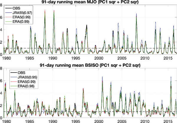
Interannual (91 day running mean) variability of the MJO and BSISO mode PC amplitudes. Values from observations (OBS) and three different reanalyses are shown. The correlation coefficients between OBS and reanalyses are shown in parentheses in the legend after each reanalysis name.

3.2 Phase composites of MJO and BSISO signals

For each MJO phase, Fig. 4 shows the event composites of intraseasonal OLR in three regions: Eastern Indian Ocean (E. IO; 85–95°E, 5°S–5°N), MC (125–135°E, 10°S–Eq), and Western Pacific (W. Pac; 165 –175°E, 10°S–Eq). The eight MJO phases are defined by the PCs. The detailed definition and the associated positions of the major convection can be found in Fig. 7 in Kikuchi et al. (2012). The procedure for identifying the event days can also be found in Kikuchi et al. (2012) (Fig. 3). The regions used for averaging are chosen based on “local convective variability maximum” based on observational EEOFs (Fig. 1a) and intraseasonal OLR spatial patterns (not shown). Here, apart from the timing, we infer if OLR from the reanalyses “converge” toward observed OLR values. The negative (positive) values correspond to MJO convectively active (suppressed) phases. Consistent with Fig. 1, JRA55 underestimates the amplitude of MJO throughout all the three regions and for all the phases, especially during the peak convective (phases 3, 5, and 7 in the three regions, respectively) and peak suppressed (phases 7, 1, and 2) ones. By contrast, ERAi and ERA5 are comparable in terms of both magnitudes and phases in all the regions. A closer look suggests that ERAi is perhaps better in phasing with observation, particularly during the peak phase of convection (phase 5) in the MC region.

Fig. 4.

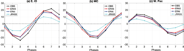
Regional averaged values over Eastern Indian Ocean (E. IO; 85–95°E, 5°S–5°N), Maritime Continent (MC; 125–135°E, 10°S–Eq), and Western Pacific (W. Pac; 165–175°E, 10°S–Eq) of OLR composites of each MJO phase from observations (OBS, in black), ERA5 (in red), ERA-interim (ERAi, in blue), and JRA55 (in light blue). Daily OLR values were bandpass-filtered (25–90 days) before constructing the composites. The period of the analysis is 1979–2016. Shading areas show the standard errors.

For BSISO, Fig. 5 shows the composites for three regions. The same longitude but different latitude centers as Fig. 4 are chosen for each region. Because of the northward propagating nature and longitudinal extent of BSISO convection (Fig. 2), phase composites in MC (Fig. 5b) and W. Pac (Fig. 5c) are almost in phase, but with a decrease in values to the east (W. Pac). Consistent with the MJO composites, in the three regions both ERA reanalyses are comparable with the observation, whereas JRA55 largely underestimates the OLR composite values. ERA5 shows the best estimates in both amplitudes and phases when compared with the observation for BSISO.

Fig. 5.

Regional averaged values over Eastern Indian Ocean (E. IO; 85–95°E, 5°S–5°N), Maritime Continent (MC; 125–135°E, 5–15°N), and Western Pacific (W. Pac; 165–175°E, 5–15°N) of OLR composites of each BSISO phase from observations (OBS, in black), ERA5 (in red), ERA-interim (ERAi, in blue), and JRA55 (in light blue). Daily OLR values were bandpass-filtered (25–90 days) before constructing the composites. The period of the analysis is 1979–2016. Shading areas show the standard errors.

Precipitation is one of the most influential ocean-forcing variables associated with ISO as it can impact the upper-ocean stability. In Indo-Pacific warm pool region, salinity is suggested to be the main controller of the upper-ocean stratification, and its modulation of upper-ocean stratification and intraseasonal SST can potentially feedback onto the ISOs (e.g., Drushka et al. 2012; Guan et al. 2014). Of the regions considered here, the intensity of both MJO and BSISO convective anomalies is higher over the E. IO (Figs. 4a, 5a). The MJO composite evolution of precipitation (Fig. 6a) suggests that all three reanalysis products underestimate the precipitation amount during “peak” phases, particularly missing the timing of “amplitude intensification”. Besides magnitude, phasing is also not well represented. For example, active peak timing occurs at phase 2 in the two ERA reanalyses and at phase 1 in JRA55, whereas it is at phase 3 in observation. Similar underestimations in precipitation amplitude and errors in MJO phasing are also noticed in the other two regions (Figs. 6b, 6c), with larger errors in the W. Pac, especially around the peak phases (phases 3 and 7 based on observation). Compared with MJO, the reanalyses better estimate the BSISO-related precipitation both the amplitudes and phases of the peaks in E. IO and W. Pac, but ERAi misses the convective peak (phase 6) in MC (Fig. 7). Nonetheless, the composite values are underestimated in all the regions during both MJO and BSISO, with ERA5 showing closer estimates to the observational values. JRA55, while showing the worst estimates in MJO composites, demonstrates better estimates in BSISO composites when compared with those of ERAi. A more quantitative discussion on these precipitation differences in both amplitudes and phases with other ISO-related variables can be found in the next section.

Fig. 6.

Eastern Indian Ocean (E. IO; 85–95°E, 5°S–5°N), Maritime Continent (MC; 125–135°E, 10°S–Eq), and Western Pacific (W. Pac; 165–175°E, 10°S–Eq) regional averaged intraseasonal precipitation composites of each MJO phase from TRMM observation (OBS), ERA5, ERA-interim (ERAi), and JRA55. The period of the analysis is 1998–2016. Shading areas show the standard errors.

Fig. 7.

Eastern Indian Ocean (E. IO; 85–95°E, 5°S–5°N), Maritime Continent (MC; 125–135°E, 5–15°N), and Western Pacific (W. Pac; 165–175°E, 5–15°N) regional averaged intraseasonal precipitation composites of each BSISO phase from TRMM observation (OBS), ERA5, ERA-interim (ERAi), and JRA55. The period of the analysis is 1998–2016. Shading areas show the standard errors.

Another diagnostic to assess regional precipitation characteristics is the probability distribution (Fig. 8). Note that the probability density functions (PDFs) were computed on the basis of bandpass-filtered daily anomalies over the regions of interest in Fig. 6 (instead of only based on MJO or BSISO event days, during which the PC amplitudes are larger than 1, as the composites in Figs. 6, 7). As the MJO propagates eastward, the shape of the PDF narrows from a higher probability of occurrences of higher amplitude days to “near-normal” days. Although the PDFs show that both ERA5 and ERAi underrepresent the number of stronger convection (as well as suppression) events, the PDFs from ERA5 are closer to observations when compared with ERAi, particularly in the E. IO region. JRA55, especially in MC and W. Pac regions, shows the closest PDFs to observation. However, it is not the case for event composites (Figs. 6, 7). This inconsistency between intraseasonal PDFs and event composites of MJO and BSISO may suggest the importance of the estimation of the timing of the events. As precipitation is strongly related to the ISO variability, the underestimations of intraseasonal variability of precipitation and errors in the peak phases may potentially influence simulations and investigation of ISOs when using the reanalysis datasets.

Fig. 8.

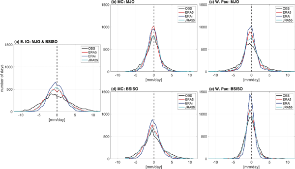
Eastern Indian Ocean [(a) E. IO; 85–95°E, 5°S–5°N for both MJO and BSISO], Maritime Continent [MC; 125–135°E, 10°S–Eq for MJO (b) and 5°N to 15°N for BSISO (d)], and Western Pacific [W. Pac; 165–175°E, 10°S–Eq for MJO (c) and 5°N to 15°N for BSISO (e)] regional averaged intraseasonal probability density function (PDF) from TRMM observation (OBS), ERA5, ERA-interim (ERAi), and JRA55. The interval used to calculate PDF was 0.5 mm day⁻¹. The period of the analysis is 1998–2016.

3.3 Biases in estimates of MJO and BSISO-related intraseasonal variables

Given that the ERA5 shows an improved representation of MJO- and BSISO-related precipitation when compared with ERAi, does this lead to corresponding improvements in other ISO-related variables (e.g., winds and other surface fluxes) that are important to ocean forcing? Moreover, given that the JRA55 shows large underestimations in amplitudes and biases in the phasing of event composites for convective-related variables (OLR and precipitation), does it also show large biases in other variables? To answer these questions, Figs. 9 and 10 show composites of the convective phases of MJO- and BSISO-related variables from observations and the corresponding errors or biases (expressed as a percentage in comparison with observations) in the reanalyses. Convective phases for each variable are chosen from the maximum regional mean values, and the observation-based peak phase for each variable is shown (in black parentheses). The phase biases in reanalyses (if any), in comparison with observations, are also shown (in brackets; color differs by reanalyses). Those percentage differences not passing the 95 % student t-test are in parentheses, suggesting the reanalysis biases (compared with observations) are not significant.

Fig. 9.

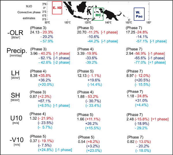
Biases of MJO convective phase-related intraseasonal values of air–sea variables from ERA5 (percentage in red), ERAi (percentage in blue), and JRA55 (percentage in light blue) in the Eastern Indian Ocean (left panel), Maritime Continent (middle panel), and Western Pacific Ocean (right panel). Percentage differences not passing the 95 % Student t-test are in parentheses. Convective phases for each variable are chosen from the maximum regional mean. Composite value and the corresponding peak phase computed on the basis of observation are shown in black for each variable. All the percentages (biases) are compared with the observational values (shown in black numbers). Phase biases (positive represents the reanalysis lagging the observation) in reanalyses (compared with observation) are shown in brackets following the percentage biases. Different periods were used for each variable depending on the availability of observation: 1979–2016 for OLR, 1998–2016 for precipitation, 1985–2016 for heat fluxes, and 1999–2009 for 10 m winds.

Fig. 10.

Biases of BSISO convective-phase related intraseasonal values of air–sea variables from ERA5 (percentage in red), ERAi (percentage in blue), and JRA55 (percentage in light blue) in Eastern Indian Ocean (left panel), Maritime Continent (middle panel), and Western Pacific Ocean (right panel). Percentage differences not passing the 95 % Student t-test are in parentheses. Convective phases for each variable are chosen from the maximum regional mean values. Composite value and the corresponding peak phase computed on the basis of observation are shown in black for each variable. All the percentages (biases) are compared with the observational values (shown in black numbers). Phase biases (positive represents the reanalysis lagging the observation) in reanalyses (compared with observation) are shown in brackets following the percentage biases. Different periods were used for each variable depending on the availability of observation: 1979–2016 for OLR, 1998–2016 for precipitation, 1985–2016 for heat fluxes, and 1999–2009 for 10 m winds. The gray text indicates the regional composite values are too small, and therefore, the biases between reanalyses and observation are not shown.

In Fig. 9, the peak amplitudes of MJO precipitation and OLR are shown to be underestimated by all three reanalyses, and the reanalyses tend to show phase biases of 1–2 phases leading the observation in E. IO and W. Pac regions for precipitation. Although the two ERA reanalyses produce better OLR composites than the JRA55, all of them show significant biases in precipitation: The underestimates in the precipitation amplitudes range from approximately 20–60, 30–70, and 40–80 %, depending on the region in ERA5, ERAi, and JRA55, respectively. Although ERA5 best represents the variability of precipitation associated with MJO convective phases in all the three regions, similar improvements in other variables are not evident. The errors in surface heat fluxes and near-surface winds compared with the observations are regionand variable- dependent. Nonetheless, ERA5 shows a better estimation than ERAi in latent heat flux in all three regions. Moreover, we note that both ERA5 and ERAi tend to underestimate near-surface (10 m) winds, although the errors in underestimating the winds are generally statistically insignificant for MJO (with parentheses in Fig. 9). The JRA55, although showing comparable bias amplitudes to ERA5 in heat fluxes and winds, tends to show phase leads (by 1 phase) in the E. IO during MJO convective phases.

For BSISO, consistent with the MJO composites, ERA5 outperforms the other two reanalyses in estimating OLR and precipitation amplitudes in all the regions (Fig. 10). However, no phase bias, except the 1 phase lagging of OLR in JRA55 in E. IO, is shown in the reanalyses for BSISO events. ERA5 also outperforms ERAi in 10 m winds in almost all the regions during BSISO convective phases. Nonetheless, a significant underestimation of 10 m zonal wind by approximately 50 % in amplitude is seen in E. IO during BSISO, accompanied with 1–2 phase biases (lagging the observation) depending on the reanalyses.

Since the suppressed phases are also crucial in terms of the ISO-related air–sea interaction, we also computed the amplitude and phase biases during suppressed phases for both MJO (Fig. 11) and BSISO (Fig. 12). The convective suppressed phases are chosen on the basis of the negative peaks for each variable. Consistent with the convective phase of MJO (Fig. 9), the amplitudes of precipitation composites show large and significant biases during MJO suppressed phases for all three reanalyses (Fig. 11). Additionally, large biases are noted in sensible heat (SH), especially in the E. IO. Besides the amplitudes, the reanalyses show larger phase biases (leading the observations) during the suppressed phases for all the variables. For JRA55, the phase biases occur in all three regions. The BSISO composites for suppressed phases (Fig. 12) are more consistent with convective phases (Fig. 10) than those of MJO, although during BSISO suppressed phases, the reanalyses show better estimates in the peak phases, with no phase biases for precipitation, SH, and winds.

Fig. 11.

Same as in Fig. 9 but shows the results for suppressed phases. Suppressed phases for each variable are chosen from the minimum (largest negative) regional mean values.

Fig. 12.

Same as in Fig. 10 but shows the results for suppressed phases. Suppressed phases for each variable are chosen from the minimum (largest negative) regional mean values.

Furthermore, despite ERAi and ERA5 not representing the amplitudes of the MJO convective peaks well especially in the E. IO, the lead–lag relationship between precipitation and the heat fluxes are similar between the ERA reanalyses and the observations (Fig. 9): the heat fluxes, specifically the latent heat flux, lags the peak of precipitation in the E. IO by approximately 5 days in observation and 10 days in the ERA reanalyses (one and two phases, respectively), and the lag decreases eastward to approximately no lag in the W. Pac. The phase relationship during MJO events is consistent with previous studies, with the latent heat flux peak lagging the OLR minimum and the rainfall peak in the Indian Ocean (e.g., Inness and Slingo 2003; Fu and Wang 2004; Duvel and Vialard 2007; DeMott et al. 2015). During the active phase of MJO, the convection system generates a maximum precipitation, accompanied by a minimum OLR. This increase in cloudiness leads to a reduction in the shortwave radiation reaching the ocean surface, as well as induces a strong westerly wind on the west side of the convective system (as part of the Rossby wave response), which then induces an increase in the surface heat fluxes, especially the latent heat flux, lagging the convection. Moreover, DeMott et al. (2015) demonstrated the SH to have almost no lag to the peak of convection (OLR), and this consistency in phase can be seen in both observation and reanalyses (Fig. 9), implying that both ERA reanalyses are suitable datasets to investigate the MJO-related flux variabilities.

We also want to note the small composite values of E. IO latent heat flux (LH) and W. Pac SH flux for BSISO. Because of the complicated movement (both northward and eastward) of BSISO convection, the LH flux is not spatially coherent with BSISO-associated OLR in the E. IO (red boxes in Fig. 13). During the strongest convection in E. IO (phase 2, during which the most negative OLR is shown), the LH shows a rather small composite value in the region. A similar relationship is also found for SH in the Pacific Ocean. In Fig. 14, although the OLR (convection or suppression) feature extends to almost the central Pacific in some phases (for example, phases 1 and 5, when OLR shows the largest values in the W. Pac box), SH shows near-zero values, given that SH is generally low over the open oceans. LH in the E.IO and SH in the E. Pac boxes both show very small values. In other words, it is hard to quantify how BSISO convection (OLR and precipitation) modulates the heat flux variability at the locations we have chosen, although OLR shows a strong signal in these regions. Overall, both ERA reanalyses estimate well the amplitudes of LH during both convective and suppressed BSISO phases, whereas larger errors are shown in SH (Figs. 10, 12). A better way of quantifying the BSISO-associated heat fluxes, however, is needed to investigate the robustness of this conclusion.

Fig. 13.

Event composites of OLR (contour) and LH (shaded) for each BSISO phase computed from observation. Numbers in parentheses show the event days for each phase. Red boxes show the region we chose for averaging for the BSISO over the E. IO.

Fig. 14.

Event composites of OLR (contour) and SH (shaded) for each BSISO phase computed from observation. The numbers in parentheses show the event days for each phase. Red boxes show the region we chose for averaging for the BSISO over the W. Pac.

4. Conclusion and discussion

Using a bimodal ISO index calculated solely from OLR, we show that although ERAi and ERA5 are comparable in representing the variability of ISO-related OLR, ERA5 demonstrates a better representation in precipitation. Both ERA5 and ERAi reasonably represent the ISO spatial patterns and magnitudes throughout its eastward propagation and northward propagation (for BSISO only) from the Indian Ocean to W. Pac. JRA55, however, severely underestimates the OLR variability (by approximately 40–60 % depending on the region and season).

Regarding precipitation, ERA5 tends to outperform the other two reanalyses in estimating the intraseasonal and event-composite magnitudes, although all the reanalyses show errors in representing phases depending on the region of interest. Although on different timescales, a previous assessment of ERA5 shows improvements in timing and the value of the diurnal precipitation in comparison with ERAi, presumably because of a better convection parameterization (Hersbach et al. 2018). Although previous studies suggest a general underestimation of the amplitude of precipitation associated with MJO events in both ERAi (e.g., Adames 2017) and ERA5 (Jiang et al. 2019; near the MC), we further quantify the underestimation in regions with strong convection through the MJO and BSISO life cycle and compare the differences between the two reanalyses in this study. Since all the three analyses show significantly large differences in precipitation with observations (largest for convective MJO phases, by approximately 20–60 % for ERA5, approximately 30–70 % for ERAi, and approximately 40–80 % for JRA55, with phase biases of 1–2 depending on the region), attention should be paid when using the precipitation variable. We also demonstrate the underestimation (overestimation) of the numbers of higher amplitude (near-normal) precipitation days in the two ERA reanalyses, whereas the PDFs computed from ERA5 are closer to observations, especially in the E. IO. Furthermore, according to the phase composites, the reanalyses are not capturing the intensification of precipitation associated with the eastward propagation of the MJO and BSISO. These misrepresentations of the peaks can be one of the causes that leads to the underestimation in the amplitude of precipitation.

Despite ERA5 showing a better representation in precipitation, it does not show a better representation than ERAi and JRA55 in some of the variables associated with MJO events, such as the SH flux in MC during both the convective and suppressed phases of MJO. This is different from our expectation as winds are strongly related to the convective systems and thus, to the precipitation. However, how the nearsurface vertical gradients of temperature and moisture, which strongly impact the surface heat fluxes, improve with an improved estimate of convection systems in ERA5 is not examined. A detailed study of the vertical structure of atmospheric moisture and heating patterns, and their association with near-surface winds as well as the fluxes is required for further explanation of the differences in the improvements between precipitation and other MJO-related variables. BSISO composites of the reanalyses, conversely, suggest a better representation of 10 m winds in ERA5 than ERAi. The spatial features of each BSISO phase, however, are more complicated, and the relationship between convection (OLR and precipitation) and other variables, especially heat fluxes, is difficult to quantify by the regional composites. Another topic worthy of investigation is how the biases in the reanalysis datasets can influence the ocean salinity and heat responses. Given that the freshwater flux, and thus, the precipitation, can strongly influence the upper-ocean salinity, which further affects the stratification and upper-ocean temperature, it is important to understand how the errors in the ISO-associated precipitation in the reanalyses impact the upper-ocean variability, and how these upper-ocean changes can feedback to the ISO.

Last but not least, there are several caveats in this study: (1) All results are based on composites, whereas individual event characteristics were not tested. (2) Only three analyses were tested. (3) Several observational variables are limited to shorter periods, and only one observational dataset for each variable was used. Different observational datasets may generate different results compared with each reanalysis, although the relationship among the reanalyses will not change. (4) Space–time evolutions of BSISO convective anomalies are complex and therefore, variability of BSISO-related variables may not be well captured by the regional composites shown here. (5) Due to the focus of this study, the possible influence from phase lag biases, especially in JRA55, on simulation of the ISOs, and how the phase biases of one variable relate to other variables was not discussed. Even with these restraints, our results quantitively show a benchmark for possible datasets used for ISO-related ocean forcing by comparing them to current available observations and suggest limitations and strengths of the new ERA5 and JRA55 reanalyses. With better spatial and temporal resolutions in the new reanalyses, our results suggest potential improvements of our understanding in simulating both MJO- and BSISO-related convections and ocean responses. For example, given the known requirements of high resolution for simulating the ISO-related reasonable ocean response, such as the diurnal variability of the upper ocean, our results suggest that the usage of the improved ERA5 estimates can potentially advance our investigation in related studies.

Acknowledgment

The authors wish to thank the editor and two anonymous reviewers for comments that greatly improved the quality of this paper. This study is funded by NOAA grant NA17OAR4310252. KK also acknowledges support from NOAA grant NA17OAR4310250. The ERA5 data are available on the ECMWF Copernicus Climate Change Service (https://cds.climate.copernicus.eu/cdsapp#!/home), and the JRA55 data are available through the Japan Meteorological Agency (https://jra.kishou.go.jp/JRA-55/index_en.html#download). All other data are obtained from the Asia-Pacific Data-Research Center (ADPRC) at the University of Hawai'i (http://apdrc.soest.hawaii.edu/).

References

•  Adames,  Á. F., 2017: Precipitation budget of the Madden-Julian oscillation. J. Atmos. Sci., 74, 1799-1817.
•  Annamalai,  H., and  J. M.  Slingo, 2001: Active/break cycles: Diagnosis of the intraseasonal variability of the Asian summer monsoon. Climate Dyn., 18, 85-102.
•  Annamalai,  H., and  K. R.  Sperber, 2005: Regional heat sources and the active and break phases of boreal summer intraseasonal (30-50 day) variability. J. Atmos. Sci., 62, 2726-2748.
•  Annamalai,  H.,  J. M.  Slingo,  K. R.  Sperber, and  K.  Hodges, 1999: The mean evolution and variability of the Asian summer monsoon: Comparison of ECMWF and NCEP-NCAR reanalyses. Mon. Wea. Rev., 127, 1157-1186.
•  Bernie,  D. J.,  S. J.  Woolnough,  J. M.  Slingo, and  E.  Guilyardi, 2005: Modeling diurnal and intraseasonal variability of the ocean mixed layer. J. Climate, 18, 1190-1202.
•  Camargo,  S. J.,  A. W.  Robertson,  A. G.  Barnston, and  M.  Ghil, 2008: Clustering of eastern North Pacific tropical cyclone tracks: ENSO and MJO effects. Geochem., Geophys., Geosyst., 9, Q06V05, doi:10.1029/2007GC001861.
•  Dee,  D. P.,  S. M.  Uppala,  A. J.  Simmons,  P.  Berrisford,  P.  Poli,  S.  Kobayashi,  U.  Andrae,  M. A.  Balmaseda,  G.  Balsamo,  P.  Bauer,  P.  Bechtold,  A. C. M.  Beljaars,  L.  van de Berg,  J.  Bidlot,  N.  Bormann,  C.  Delsol,  R.  Dragani,  M.  Fuentes,  A. J.  Geer,  L.  Haimberger,  S. B.  Healy,  H.  Hersbach,  E. V.  Hólm,  L.  Isaksen,  P.  Kållberg,  M.  Köhler,  M.  Matricardi,  A. P.  McNally,  B. M.  Monge-Sanz,  J.-J.  Morcrette,  B.-K.  Park,  C.  Peubey,  P.  de Rosnay,  C.  Tavolato,  J.-N.  Thépaut, and  F.  Vitart, 2011: The ERA-interim reanalysis: Configuration and performance of the data assimilation system. Quart. J. Roy. Meteor. Soc., 137, 553-597.
•  DeMott,  C. A.,  N. P.  Klingaman, and  S. J.  Woolnough, 2015: Atmosphere-ocean coupled processes in the Madden-Julian oscillation. Rev. Geophys., 53, 1099-1154.
•  Drushka,  K.,  J.  Sprintall,  S. T.  Gille, and  S.  Wijffels, 2012: In situ observations of Madden-Julian oscillation mixed layer dynamics in the Indian and western Pacific Oceans. J. Climate, 25, 2306-2328.
•  Duvel,  J. P., and  J.  Vialard, 2007: Indo-Pacific sea surface temperature perturbations associated with intraseasonal oscillations of tropical convection. J. Climate, 20, 3056-3082.
•  Fu,  X., and  B.  Wang, 2004: The boreal-summer intraseasonal oscillations simulated in a hybrid coupled atmosphere-ocean model. Mon. Wea. Rev., 132, 2628-2649.
•  Fu,  X.,  B.  Wang,  Q. Bao P.  Liu, and  J.-Y.  Lee, 2009: Impacts of initial conditions on monsoon intraseasonal forecasting. Geophys. Res. Lett., 36, L08801, doi:10.1029/2009GL037166.
•  Graham,  R. M.,  S. R.  Hudson, and  M.  Maturilli, 2019: Improved performance of ERA5 in Arctic gateway relative to four global atmospheric reanalyses. Geophys. Res. Lett., 46, 6138-6147.
•  Guan,  B.,  T.  Lee,  D. J.  Halkides, and  D. E.  Waliser, 2014: Aquarius surface salinity and the Madden-Julian Oscillation: The role of salinity in surface layer density and potential energy. Geophys. Res. Lett., 41, 2858-2869.
•  Harada,  Y.,  H.  Kamahori,  C.  Kobayashi,  H.  Endo,  S.  Kobayashi,  Y.  Ota,  H.  Onoda,  K.  Onogi,  K.  Miyaoka, and  K.  Takahashi, 2016: The JRA-55 reanalysis: Representation of atmospheric circulation and climate variability. J. Meteor. Soc. Japan, 94, 269-302.
•  Hendon,  H. H., and  M. L.  Salby, 1994: The life cycle of the Madden-Julian oscillation. J. Atmos. Sci., 51, 2225-2237.
•  Hersbach,  H.,  P.  de Rosnay,  B.  Bell,  D.  Schepers,  A.  Simmons,  C.  Soci,  S.  Abdalla,  M.  Alonso-Balmaseda,  G.  Balsamo,  P.  Bechtold,  P.  Berrisford,  J.-R.  Bidlot,  E.  de Boisséson,  M.  Bonavita,  P.  Browne,  R.  Buizza,  P.  Dahlgren,  D.  Dee,  R.  Dragani,  M.  Diamantakis,  J.  Flemming,  R.  Forbes,  A. J.  Geer,  T.  Haiden,  E.  Hólm,  L.  Haimberger,  R.  Hogan,  A.  Horányi,  M.  Janiskova,  P.  Laloyaux,  P.  Lopez,  J.  Munoz-Sabater,  C.  Peubey,  R.  Radu,  D.  Richardson,  J.-N.  Thépaut,  F.  Vitart,  X.  Yang,  E.  Zsótér, and  H.  Zuo, 2018: Operational global reanalysis: Progress, future directions and synergies with NWP. ERA Report Series, 27, 65 pp. [Available at https://www.ecmwf.int/node/18765.]
•  Hersbach,  H.,  B.  Bell,  P.  Berrisford,  S.  Hirahara,  A.  Horányi,  J.  Muñoz-Sabater,  J.  Nicolas,  C.  Peubey,  R.  Radu,  D.  Schepers,  A.  Simmons,  C.  Soci,  S.  Abdalla,  X.  Abellan,  G.  Balsamo,  P.  Bechtold,  G.  Biavati,  J.  Bidlot,  M.  Bonavita,  G.  De Chiara,  P.  Dahlgren,  D.  Dee,  M.  Diamantakis,  R.  Dragani,  J.  Flemming,  R.  Forbes,  M.  Fuentes,  A.  Geer,  L.  Haimberger,  S.  Healy,  R. J.  Hogan,  E.  Hólm,  M.  Janisková,  S.  Keeley,  P.  Laloyaux,  P.  Lopez,  C.  Lupu,  G.  Radnoti,  P.  de Rosnay,  I.  Rozum,  F.  Vamborg,  S.  Villaume, and  J.-N.  Thépaut, 2020: The ERA5 global reanalysis. Quart. J. Roy. Meteor. Soc., 146, 1999-2049.
•  Higgins,  R. W., and  W.  Shi, 2001: Intercomparison of the principal modes of interannual and intraseasonal variability of the North American Monsoon System. J. Climate, 14, 403-417.
•  Hung,  M.-P.,  J.-L.  Lin,  W.  Wang,  D.  Kim,  T.  Shinoda, and  S. J.  Weaver, 2013: MJO and convectively coupled equatorial waves simulated by CMIP5 climate models. J. Climate, 26, 6185-6214.
•  Inness,  P. M., and  J. M.  Slingo, 2003: Simulation of the Madden-Julian oscillation in a coupled general circulation model. Part I: Comparison with observations and an atmosphere-only GCM. J. Climate, 16, 345-364.
•  Jiang,  X.,  D. E.  Waliser,  P. K.  Xavier,  J.  Petch,  N. P.  Klingaman,  S. J.  Woolnough,  B.  Guan,  G.  Bellon,  T.  Crueger,  C.  DeMott,  C.  Hannay,  H.  Lin,  W.  Hu,  D.  Kim,  C.-L.  Lappen,  M.-M.  Lu,  H.-Y.  Ma,  T.  Miyakawa,  J. A.  Ridout,  S. D.  Schubert,  J.  Scinocca,  K.-H.  Seo,  E.  Shindo,  X.  Song,  C.  Stan,  W.-L.  Tseng,  W.  Wang,  T.  Wu,  X.  Wu,  K.  Wyser,  G. J.  Zhang, and  H.  Zhu, 2015: Vertical structure and physical processes of the Madden-Julian oscillation: Exploring key model physics in climate simulations. J. Geophys. Res.: Atmos., 120, 4718-4748.
•  Jiang,  X.,  H.  Su, and  D. E.  Waliser, 2018: Barrier effect of the Maritime Continent on the MJO: Perspectives from the large-scale control and local topographic effect. Proceeding of American Geophysical Union, Fall Meeting 2018, Washington D.C., Abstract #A24F-01, American Geophysical Union.
•  Jiang,  X.,  H.  Su, and  D. E.  Waliser, 2019: A damping effect of the Maritime Continent for the Madden-Julian Oscillation. J. Geophys. Res.: Atmos., 124, 13693-13713.
•  Jiang,  X.,  Á. F.  Adames,  D.  Kim,  E. D.  Maloney,  H.  Lin,  H.  Kim,  C.  Zhang,  C. A.  DeMott, and  N. P.  Klingaman, 2020: Fifty years of research on the Madden-Julian Oscillation: Recent progress, challenges, and perspectives. J. Geophys. Res.: Atmos., 125, e2019JD030911, doi:10.1029/2019JD030911.
•  Jones,  C.,  L. M. V.  Carvalho,  R. W.  Higgins,  D. E.  Waliser, and  J.-K. E.  Schemm, 2004: Climatology of tropical intraseasonal convective anomalies: 1979-2002. J. Climate, 17, 523-539.
•  Julian,  P. R., and  R.  Madden, 1981: Comments on a paper by T. Yasunari, a quasi-stationary appearance of 30 to 40-day period in the cloudiness fluctuations during the summer monsoon over India. J. Meteor. Soc. Japan, 59, 435-437.
•  Kayano,  M. T., and  V. E.  Kousky, 1999: Intraseasonal (30-60 day) variability in the global tropics: Principal modes and their evolution. Tellus A, 51, 373-386.
•  Kessler,  W. S., 2001: EOF representations of the Madden–Julian oscillation and its connection with ENSO. J. Climate, 14, 3055-3061.
•  Kikuchi,  K., 2020: Extension of the bimodal intraseasonal oscillation index using JRA-55 reanalysis. Climate Dyn., 54, 919-933.
•  Kikuchi,  K., and  B.  Wang, 2010: Formation of tropical cyclones in the northern Indian Ocean associated with two types of tropical intraseasonal oscillation modes. J. Meteor. Soc. Japan, 88, 475-496.
•  Kikuchi,  K.,  B.  Wang, and  Y.  Kajikawa, 2012: Bimodal representation of the tropical intraseasonal oscillation. Climate Dyn., 38, 1989-2000.
•  Kiladis,  G. N.,  J.  Dias,  K. H.  Straub,  M. C.  Wheeler,  S. N.  Tulich,  K.  Kikuchi,  K. M.  Weickmann, and  M. J.  Ventrice, 2014: A comparison of OLR and circulationbased indices for tracking the MJO. Mon. Wea. Rev., 142, 1697-1715.
•  Kim,  H.-M.,  C. D.  Hoyos,  P. J.  Webster, and  I.-S.  Kang, 2008: Sensitivity of MJO simulation and predictability to sea surface temperature variability. J. Climate, 21, 5304-5317.
•  Knutson,  T. R., and  K. M.  Weickmann, 1987: 30–60 day atmospheric oscillations: Composite life cycles of convection and circulation anomalies. Mon. Wea. Rev., 115, 1407-1436.
•  Kobayashi,  S.,  Y.  Ota,  Y.  Harada,  A.  Ebita,  M.  Moriya,  H.  Onoda,  K.  Onogi,  H.  Kamahori,  C.  Kobayashi,  H.  Endo,  K.  Miyaoka, and  K.  Takahashi, 2015: The JRA-55 reanalysis: General specifications and basic characteristics. J. Meteor. Soc. Japan, 93, 5-48.
•  Krishnamurti,  T. N.,  D. K.  Oosterhof, and  A. V.  Mehta, 1988: Air-sea interaction on the timescale of 30 to 50 days. J. Atmos. Sci., 45, 1304-1322.
•  Kummerow,  C.,  W.  Barnes,  T.  Kozu,  J.  Shiue, and  J.  Simpson, 1998: The Tropical Rainfall Measuring Mission (TRMM) sensor package. J. Atmos. Oceanic Technol., 15, 809-817.
•  Lau,  K.-M., and  P. H.  Chan, 1985: Aspects of the 40-50 day oscillation during the northern winter as inferred from outgoing longwave radiation. Mon. Wea. Rev., 113, 1889-1909.
•  Li,  Y.,  W.  Han,  W.  Wang,  L.  Zhang, and  M.  Ravichandran, 2018: The Indian summer monsoon intraseasonal oscillations in CFSv2 forecasts: Biases and importance of improving air-sea interaction processes. J. Climate, 31, 5351-5370.
•  Liebmann,  B., and  C. A.  Smith, 1996: Description of a complete (interpolated) outgoing longwave radiation dataset. Bull. Amer. Meteor. Soc., 77, 1275-1277.
•  Lorenz,  D. J., and  D. L.  Hartmann, 2006: The effect of the MJO on the North American monsoon. J. Climate, 19, 333-343.
•  Madden,  R. A., 1986: Seasonal variations of the 40-50 day oscillation in the tropics. J. Atmos. Sci., 43, 3138-3158.
•  Maloney,  E. D., and  D. L.  Hartmann, 1998: Frictional moisture convergence in a composite life cycle of the Madden-Julian oscillation. J. Climate, 11, 2387-2403.
•  Maloney,  E. D., and  D. L.  Hartmann, 2000a: Modulation of eastern north Pacific hurricanes by the Madden–Julian oscillation. J. Climate, 13, 1451-1460.
•  Maloney,  E. D., and  D. L.  Hartmann, 2000b: Modulation of hurricane activity in the Gulf of Mexico by the Madden-Julian oscillation. Science, 287, 2002-2004.
•  Raymond,  D. J.,  S. L.  Sessions,  A. H.  Sobel, and  Ž.  Fuchs, 2009: The mechanics of gross moist stability. J. Adv. Model. Earth Syst., 1, 9, doi:10.3894/JAMES.2009.1.9.
•  Reynolds,  R. W.,  T. M.  Smith,  C.  Liu,  D. B.  Chelton,  K. S.  Casey, and  M. G.  Schlax, 2007: Daily high-resolution-blended analyses for sea surface temperature. J. Climate, 20, 5473-5496.
•  Riley Dellaripa,  E. M., and  E. D.  Maloney, 2015: Analysis of MJO wind-flux feedbacks in the Indian Ocean using RAMA buoy observations. J. Meteor. Soc. Japan, 93A, 1-20.
•  Salby,  M. L., and  H. H.  Hendon, 1994: Intraseasonal behavior of clouds, temperature, and motion in the tropics. J. Atmos. Sci., 51, 2207-2224.
•  Sharmila,  S.,  P. A.  Pillai,  S.  Joseph,  M.  Roxy,  R. P. M.  Krishna,  R.  Chattopadhyay,  S.  Abhilash,  A. K.  Sahai, and  B. N.  Goswami, 2013: Role of ocean–atmosphere interaction on northward propagation of Indian summer monsoon intra-seasonal oscillations (MISO). Climate Dyn., 41, 1651-1669.
•  Shinoda,  T.,  H. H.  Hendon, and  J.  Glick, 1999: Intraseasonal surface fluxes in the tropical western Pacific and Indian Oceans from NCEP reanalyses. Mon. Wea. Rev., 127, 678-693.
•  Slingo,  J. M.,  K. R.  Sperber,  J. S.  Boyle,  J.-P.  Ceron,  M.  Dix,  B.  Dugas,  W.  Ebisuzaki,  J.  Fyfe,  D.  Gregory,  J.-F.  Gueremy,  J.  Hack,  A.  Harzallah,  P.  Inness,  A.  Kitoh,  W. K.-M.  Lau,  B.  McAvaney,  R.  Madden,  A.  Matthews,  T. N.  Palmer,  C.-K.  Parkas,  D.  Randall, and  N.  Renno, 1996: Intraseasonal oscillations in 15 atmospheric general circulation models: Results from an AMIP diagnostic subproject. Climate Dyn., 12, 325-357.
•  Sobel,  A. H.,  E. D.  Maloney,  G.  Bellon, and  D. M.  Frierson, 2010: Surface fluxes and tropical intraseasonal variability: A reassessment. J. Adv. Model. Earth Syst., 2, 2, doi:10.3894/JAMES.2010.2.2.
•  Straub,  K. H., 2013: MJO initiation in the real-time multivariate MJO index. J. Climate, 26, 1130-1151.
•  Székely,  E.,  D.  Giannakis, and  A. J.  Majda, 2016: Extraction and predictability of coherent intraseasonal signals in infrared brightness temperature data. Climate Dyn., 46, 1473-1502.
•  Tian,  B.,  D. E.  Waliser,  E. J.  Fetzer,  B. H.  Lambrigtsen,  Y. L.  Yung, and  B.  Wang, 2006: Vertical moist thermodynamic structure and spatial-temporal evolution of the MJO in AIRS observations. J. Atmos. Sci., 63, 2462-2485.
•  Ventrice,  M. J.,  M. C.  Wheeler,  H. H.  Hendon,  C. J.  Schreck III,  C. D.  Thorncroft, and  G. N.  Kiladis, 2013: A modified multivariate Madden-Julian oscillation index using velocity potential. Mon. Wea. Rev., 141, 4197-4210.
•  Wang,  B., and  H.  Rui, 1990: Synoptic climatology of transient tropical intraseasonal convection anomalies: 1975–1985. Meteor. Atmos. Phys., 44, 43-61.
•  Wang,  J.,  W.  Wang,  X.  Fu, and  K.-H.  Seo, 2012: Tropical intraseasonal rainfall variability in the CFSR. Climate Dyn., 38, 2191-2207.
•  Wang,  S.,  D.  Ma,  A. H.  Sobel, and  M. K.  Tippett, 2018: Propagation characteristics of BSISO indices. Geophys. Res. Lett., 45, 9934-9943
•  Wang,  W.,  M.  Chen, and  A.  Kumar, 2009: Impacts of ocean surface on the northward propagation of the boreal summer intraseasonal oscillation in the NCEP Climate Forecast System. J. Climate, 22, 6561-6576.
•  Weare,  B. C., and  J. S.  Nasstrom, 1982: Examples of extended empirical orthogonal function analyses. Mon. Wea. Rev., 110, 481-485.
•  Webster,  P. J.,  V. O.  Magaña,  T. N.  Palmer,  J.  Shukla,  R. A.  Tomas,  M.  Yanai, and  T.  Yasunari, 1998: Monsoons: Processes, predictability, and the prospects for prediction. J. Geophys. Res., 103, 14451-14510.
•  Wheeler,  M. C., and  H. H.  Hendon, 2004: An all-season real-time multivariate MJO index: Development of an index for monitoring and prediction. Mon. Wea. Rev., 132, 1917-1932.
•  Yamaura,  T., and  Y.  Kajikawa, 2017: Decadal change in the boreal summer intraseasonal oscillation. Climate Dyn., 48, 3003-3014.
•  Yasunari,  T., 1979: Cloudiness fluctuations associated with the Northern Hemisphere summer monsoon. J. Meteor. Soc. Japan, 57, 227-242.
•  Yu,  L.,  R. A.  Weller, and  B.  Sun, 2004: Improving latent and sensible heat flux estimates for the Atlantic Ocean (1988-99) by a synthesis approach. J. Climate, 17, 373-393.
•  Zhang,  C., 2005: Madden-Julian Oscillation. Rev. Geophys., 43, RG2003, doi:10.1029/2004RG000158.
•  Zhang,  C., and  J.  Gottschalck, 2002: SST anomalies of ENSO and the Madden-Julian oscillation in the equatorial Pacific. J. Climate, 15, 2429-2445.
•  Zhang,  C., and  M.  Dong, 2004: Seasonality in the Madden-Julian oscillation. J. Climate, 17, 3169-3180.
•  Zhang,  C.,  M.  Dong,  S.  Gualdi,  H. H.  Hendon,  E. D.  Maloney,  A.  Marshall,  K. R.  Sperber, and  W.  Wang, 2006: Simulations of the Madden-Julian Oscillation in four pairs of coupled and uncoupled global models. Climate Dyn., 27, 573-592.