Review and Further Validation of a Practical Single-Particle Breakage Model

Abstract

Particle breakage occurs in comminution machines and, inadvertently, in other process equipment during handling as well as in geotechnical applications. For nearly a century, researchers have developed mathematical expressions to describe single-particle breakage having different levels of complexity and abilities to represent it. The work presents and analyses critically a breakage model that has been found to be suitable to describe breakage of brittle materials in association to the discrete element method, either embedded in it as part of particle replacement schemes or coupled to it in microscale population balance models. The energy-based model accounts for variability and size-dependency of fracture energy of particles, weakening when particles are stressed below this value, as well as energy and size-dependent fragment size distributions when particles are stressed beyond it, discriminating between surface and body breakage. The work then further validates the model on the basis of extensive data from impact load cell and drop weight tests. Finally, a discussion of challenges associated to fitting its parameters and on applications is presented.

1. Introduction

Single-particle breakage tests have long been used to analyze fracture phenomena (Arbiter et al., 1969; Schönert, 1972; Rumpf, 1973), study energy utilization in comminution processes (Rumpf, 1973; Schubert, 1987; Dan and Schubert, 1990; Tavares, 1999), analyze the effect of particle size, shape, material properties and modes of loading on particle breakage characteristics (Yashima et al., 1987; Tavares and King, 1998; Rozenblat et al., 2012; Saeidi et al., 2016; Saeidi et al., 2017; Lois-Morales et al., 2020), investigate energy-size reduction relationships (Piret, 1953; Bergstrom et al., 1961; Rumpf, 1973; Narayanan and Whiten, 1988; Morrell, 2004) and analyze material deformation response under applied stresses (Schönert, 1991; Sikong et al., 1990; Tavares and Almeida, 2020).

One application of single-particle breakage information that has grown significantly in recent decades has been to support mathematical models of comminution and mechanical degradation during handling. This information was initially used as part of phenomenological models of comminution devices, including ball mills, autogenous and semi-autogenous mills and cone crushers (Narayanan and Whiten, 1988; Napier-Munn et al., 1996), as well as of degradation during handling (Teo et al., 1990; Weedon and Wilson, 2000), although originally in a fairly simplistic way. Perhaps influenced by the conditions used in the standardized twin pendulum, and later also in the drop weight tester (JKDWT) by the Julius Kruttschnitt Mineral Research Centre (JKMRC) (Napier-Munn et al., 1996), attention was initially only given to the relationship between the energy applied and the resulting fragmentation at relatively high specific impact energies.

From the beginning of the 1990s, research on the discrete element method (DEM) applied to tumbling mills (Mishra and Rajamani, 1992; King and Bourgeois, 1993; Morrison and Cleary, 2004) has demonstrated that very few impacts occur at the high specific energies that are object of testing in the JKDWT, and that the majority of collisions occur at impact energies that are either able to only impose limited breakage to particles or break them only after repeated stressing. This led to recognition of the importance of deepening the investigation of conditions that result in primary breakage, including breakage probability, weakening by repeated impacts and progeny size distributions at very low specific impact energies (Tavares, 2007). This shed new light into the subject, which had been object of relatively scattered studies before then (Rumpf, 1973; Baumgardt et al., 1975; Krogh, 1980; Schönert, 1979; Yashima et al., 1987). Nevertheless, the importance of very low energy impacts was recognized over 70 years ago by Fred Bond, when developing the standard crushability test (Bond, 1947), in which particles are repeatedly stressed at increasing impact energies until primary breakage occurs (Tavares and Carvalho, 2007).

A definition that has a central role when dealing with particle breakage is that of particle fracture energy (Baumgardt et al., 1975; King and Bourgeois, 1993). It corresponds to the stressing energy below which the core of the particle is maintained unbroken, whereas potentially damaged, while the surface of the particle may lose mass due to abrasion-like breakage when it is subjected to a stressing event. This particle fracture energy varies from particle to particle as well as with particle size and defines the threshold between massive or body breakage at higher impact energies and surface breakage that occurs at lower stressing energies (Tavares and King, 1998).

As mathematical models of different mills, crushers and handling systems evolved, incorporating information from DEM, it became evident that more detailed information on particle breakage was necessary. It is worth mentioning that several approaches circumvented the need for this information by either using data from particle bed breakage tests (Datta and Rajamani, 2002) or from the process itself, by back-calculating the selection function from data (Capece et al., 2014; Wang et al., 2012). However, they are not as generally applicable given their more limited ability to decouple material from process (Tavares, 2017). As such, the most powerful approaches used in advanced mathematical models and simulations are particle-based, that is, require information on how individual particles respond to stresses, either when they are fully resolved in the DEM simulation or when they are not. It is important to recognize that in order to be useful in such models, particle response must be known under the variety of conditions to which it will be subjected to in a comminution device or a system that can cause mechanical degradation. These typically include widely varied particle sizes, stressing intensities, geometries and rates of stressing as well as modes of stress application.

A fairly large number of mathematical models describing particle breakage has been proposed in the literature, which may be potentially of use in association to advanced mathematical models and DEM simulations. In most of them the variable of interest is the stressing energy (Tavares and King, 1998; Vogel and Peukert, 2003; Morrison et al., 2007; Bonfils, 2017; Ballantyne et al., 2017), whereas in a few the variable of interest is impact velocity (Ghadiri and Zhang, 2002; Rozenblat et al., 2012) or force (Rodnianski et al., 2019). Also, several of these models have been proposed that relate the size distribution of fragments to the stressing energy applied, not discriminating between volume or surface breakage (Ballantyne et al., 2017; Ouchterlony and Sanchidrián, 2018). These models, however, are not meant to discriminate particles individually, being only suited to describe the response of the entire batch. Other models have been proposed to describe the so-called incremental breakage, lumping together surface breakage and weakening by repeated stressing (Morrison et al., 2007; Bonfils et al., 2016), being very limited when used in association to advanced mathematical models of comminution and degradation. Yet other models focused exclusively on surface breakage (Ghadiri and Zhang, 2002).

The present work analyzes critically and also presents further evidence of the validity of a comprehensive mathematical model proposed by the author and his co-workers over the last 25 years (Tavares, 1997; Tavares and King, 1998; Tavares and King, 2002; Tavares, 2009; Carvalho et al., 2015; Tavares and Chagas, 2021) and schematically shown in Fig. 1 to describe several aspects of particle breakage.

Fig. 1

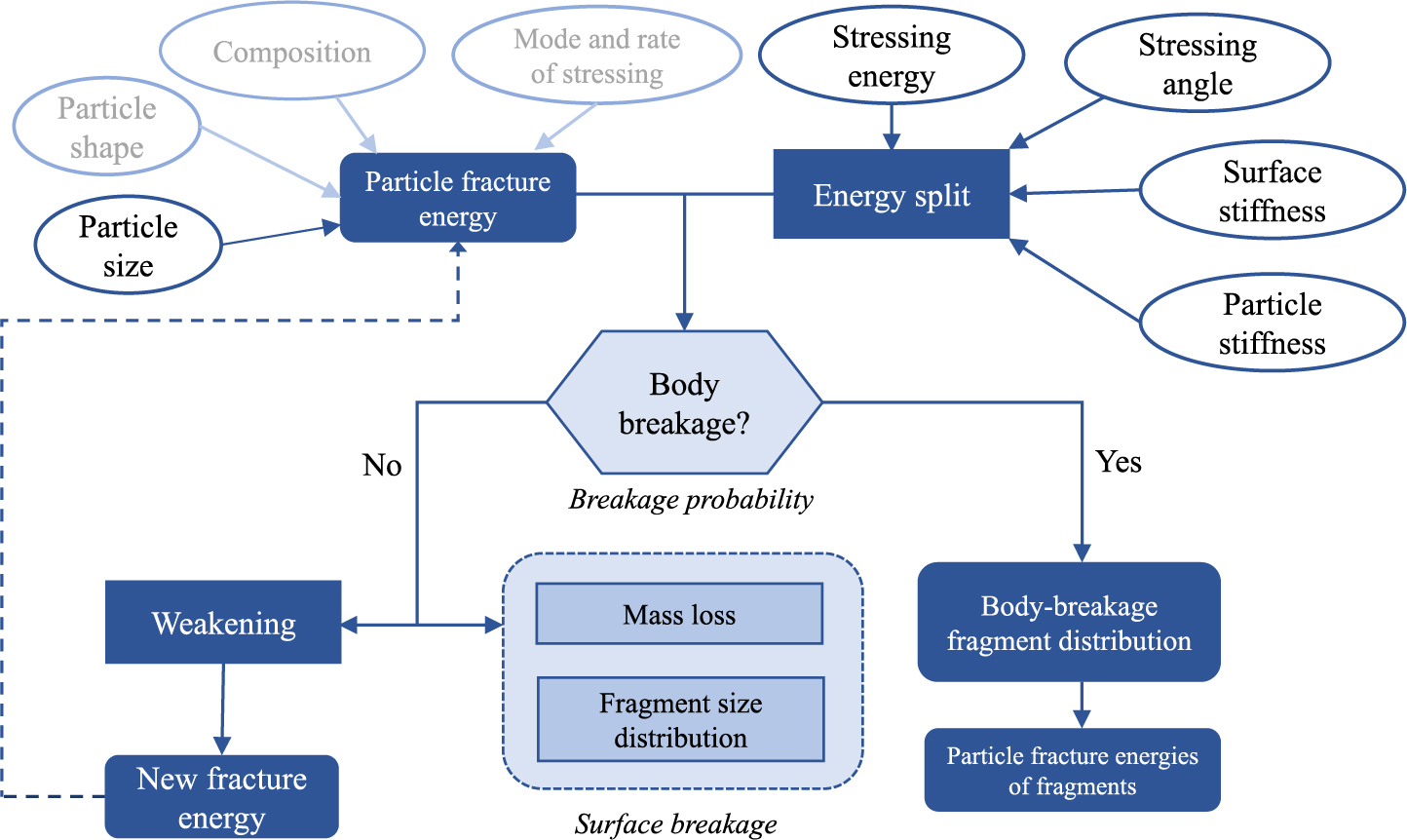
General scheme of the breakage model.

2. Breakage probability

2.1 Body breakage probability distributions

Arguably, the central part of the model is the breakage probability (Fig. 1). It represents the relationship between the applied stressing energy and the resulting proportion of particles that have undergone body or massive breakage when particles contained in a batch are stressed under identical conditions. Breakage in this context is defined arbitrarily as loss of at least 10 % of the particle mass (Dan and Schubert, 1990; Tavares, 2007). Estimates of breakage probability may be obtained experimentally from tests in which lots of particles contained in narrow size ranges are subjected to impacts by propelling them, one-by-one, against a target at a controlled velocity or dropping them under gravity. In this case the mass-specific impact energy is given by   

$$E_k=\frac{{\overline{v}}^2}{2}$$(1)

where $\overline{v}$ is the average velocity at the instant of collision against the target, which can be obtained, for instance, from measurements using a high-speed camera (Cavalcanti et al., 2021).

Alternatively, an estimate of breakage probability may be obtained by impacting particles using a drop weight tester. Assuming no loss of momentum during drop of the impactor (free-fall), the specific impact energy may be given by   

$$E_k=\frac{m\hspace{0.17em}g\hspace{0.17em}h}{{\overline{m}}_{\text{p}}}$$(2)

where m is the mass of the drop weight, ${\overline{m}}_{\text{p}}$ is the average weight of particles in the lot tested, g the acceleration due to gravity and h the net drop height, that is, the distance between the bottom of the striker and the top of the particle.

In either case, the estimate of breakage probability for a given mass-specific impact energy E is given by the proportion broken, represented by the ratio   

$$P(E_k)=\frac{N_{\text{b}}}{N}$$(3)

where N is the number of stressed particles and N_b is the number of particles that underwent body breakage as a result of application of the specific impact energy E_k. Although Eqn. (3) relates numbers of particles, it is assumed to be equivalent to the mass-based probability, given their narrow size range. In order to remove ambiguity in identifying which particles underwent breakage during execution of the test, each should be weighed individually prior to the test and also after each impact, to verify if loss of at least 10 % of their mass occurred. The measurement after the impact becomes obviously unnecessary if the particle suffered evident disintegration.

Either when particles are projected against a target or when a drop weight impacts individual particles, the specific impact energy E_k is actually a random variable, subjected to variability owing to the velocity of impact and, in the case of the later, also due to variability in particle weight. In addition to that, the proportion broken given by Eqn. (3) is only an estimate of the breakage probability, with the uncertainty reducing as the number of test-particles increase, provided no bias existed in selecting particles for the test. The magnitude of the sampling error has been estimated (Tavares, 2009) on the basis of the Binomial distribution, so that the confidence interval for the proportion broken is given by   

$$\frac{N_{\text{b}}}{N}\pm z\left(\frac{\alpha }{2}\right)\sqrt{\frac{\frac{N_{\text{b}}}{N}\left(1-\frac{N_{\text{b}}}{N}\right)}{N}}$$(4)

where α is the significance and z is the reduced Gaussian distribution.

An example of data collected following this approach is presented in Fig. 2. Obtained from impact of iron ore pellets against a target, it exhibits the typical S shape and asymmetry, evident from the skewness of the distribution to the right.

Fig. 2

Proportion broken as a function of specific impact energy from propelling fired iron ore pellets contained in the size range 12.5–9.0 mm against a steel target (data from Cavalcanti et al., 2021). Vertical error bars are given by Eqn. (4) and horizontal error bars were estimated from measurements of impact velocity using a high-speed camera.

A more direct and less time-consuming approach is to measure directly the energy required to break individual particles, using either slow compression devices (Sikong et al., 1990; Tavares, 2007; Rozenblat et al., 2011; Ribas et al., 2014; Campos et al., 2021) or instrumented drop weight test devices, such as the impact load cell (King and Bourgeois, 1993; Tavares and King, 1998; Bonfils, 2017; Lois-Morales et al., 2020), analyzing the distribution of data. While requiring more specialized equipment, this approach has the advantage of demanding significantly smaller sample volumes. In this approach, the force-deformation profile during loading of each particle is recorded and the mass-specific particle fracture energy E is given by numerical integration of the curve up to the deformation or force responsible for fracture   

$$E=\frac{1}{m_{\text{p}}}{\int }_0^{{\mathit{\Delta }}_{\text{c}}}F\hspace{0.17em}\text{d}\mathit{\Delta }$$(5)

where m_p is the weight of each individual particle, F the load, whereas Δ and Δ_c are the deformations and the deformation at primary fracture, respectively.

Typically, data in these tests present large variability (Tavares and King, 1998), so that they should be properly analyzed. A convenient method is order statistics, through which the test results are ranked in ascending order and the values i = 1, 2, …, N assigned to the ranked observations, where N is the total number of valid tests performed. The cumulative probability distribution estimates for the particle fracture energy are given by

  

$$P(E_i)=\frac{i-0.5}{N}$$(6)

An example of this type of data is shown in Fig. 3 from impact-breakage of quartz particles. Different probability distributions have been proposed over the years to describe data such as in Figs. 2 and 3, including the lognormal and upper truncated lognormal (Baumgardt et al., 1975; King and Bourgeois, 1993; Tavares and King, 1998; Tavares and King, 2002), the logistic and log-logistic (Vervoorn and Austin, 1990; Rozenblat et al., 2011; 2012), the gamma (Cavalcanti and Tavares, 2019) and the Weibull distribution (Weichert, 1992; Salman et al., 2002; Vogel and Peukert, 2004), just to name a few that have been used to fit such data (Cavalcanti and Tavares, 2018). These distributions are typically skewed to the right, with either two or three parameters and with or without a clear upper limiting (truncation) value. Fig. 3 compares some of the distributions to data. In particular when dealing with data from proportion broken, in which results only from relatively a limited number of stressing energies are available (Fig. 2), several distributions may provide fairly similar fit (Tavares, 1997), so that the selection of the most suitable distribution is not straightforward but is often not critical either. Differences in fit provided by the distribution functions are typically limited to the extremes (tails) of the data. In particular, the lower tail of the distribution, represented by the particles that are more amenable to breakage, is particularly important when describing degradation due to handling (Cavalcanti et al., 2021). On the other hand, the accurate description of the upper part of the distribution, in particular for the coarser particles, is particularly critical when using the model to predict breakage in tumbling mills, since it will determine the likelihood that particles will remain unbroken in spite of the collisions in the mill (Tavares and Carvalho, 2009).

Fig. 3

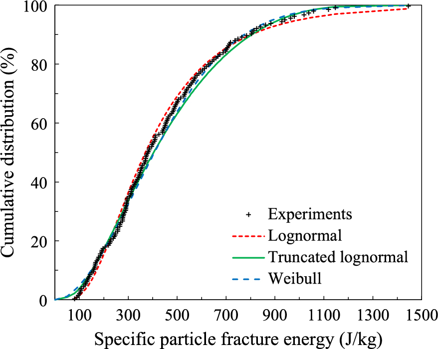
Distribution of fracture energies from impact of 200 quartz particles contained in the size range 1.18–1.0 mm in the impact load cell device. Data from Tavares (1997).

A distribution that has demonstrated to be able to describe well the variability of the data is the upper truncated lognormal distribution, given by   

$$P(E)=\frac{1}{2}\left[1+\text{erf}\left(\frac{\text{ln\hspace{0.17em}}{E}^{*}-\text{ln\hspace{0.17em}}{E}_{50}}{\sqrt{2{\sigma }^2}}\right)\right]$$(7)

and   

$$E^{*}=\frac{E_{\text{max}}\hspace{0.17em}E}{E_{\text{max}}-E}$$(8)

where P(E) represents the breakage probability or the cumulative distribution, E is the mass-specific fracture energy of the particle, which corresponds to the maximum stressing energy that it can sustain in a collision and not break, E_max is the upper truncation value of the distribution, E₅₀ and σ² are the median and the variance of the distribution, respectively. The upper truncation value is often represented by the ratio E_max/E₅₀. In the case when this ratio is equal to infinity, E* = E and Eqn. (7) becomes the lognormal distribution.

Besides stressing energy, several other variables also influence breakage probability (Fig. 1). The stiffness of the surface in contact is such a variable, which is analyzed in greater detail in 2.2, whereas the important effect of particle size is analyzed in section 2.3. The effect of impact angle on the breakage probability has been the object of some studies (Dan and Schubert, 1990; Salman et al., 2003; Tavares et al., 2018; Cavalcanti et al., 2021). In a comprehensive campaign of experiments in which iron pellets were propelled against a target (Tavares et al., 2018; Cavalcanti et al., 2021) it was found that breakage probability, and therefore body breakage, may be described considering only the normal component of the impact velocity, at least for impacts at angles that range from 90° (normal) to 30°. The effects of other variables, such as particle shape, stressing rate and mode of stressing (single or double) (Fig. 1) have been studied in the literature (Tavares, 2007; Bonfils, 2017; Saeidi et al., 2017; Lois-Morales et al., 2020) but the lack of a proper understanding on how they affect the several aspects of breakage for brittle materials in general made it impossible to properly account for them in the model. As such, it is advised that the user fits the model parameters using data that most closely match conditions that dominate in the device that is meant to be simulated.

Adapting Eqns. (7) and (8) to be used to describe discrete particles, such as those embedded in a DEM simulation (Tavares et al., 2020b; 2021) is quite straightforward, since it only requires randomly sampling the distribution every time a particle is created.

2.2 Effect of stiffness on body breakage probability

Analyzes in section 2.1 assumed that the stiffness of a particle is significantly smaller than that of the surface of the testing device or machine which is in contact with the particle. In several instances, however, that is not the case, so that a correction must be used. Given the local nature of the contacts involving application of stresses to particles and assuming validity of the Hertz contact theory (Tavares and King, 1998; Tavares et al., 2021), the proportion e of the stressing energy involved in any given event that is used to deform the particle is given by (Becker et al., 2001; Tavares and Carvalho, 2011; Tavares et al., 2021)   

$$e=\frac{1}{1+k_{\text{p}}/k_{\text{s}}}$$(9)

where k_p is the particle stiffness (Tavares and King, 1998), k_s is the Hertzian stiffness of the surface in contact with the particle. For instance, Eqn. (9) may be used to estimate the proportion of the energy recorded using Eqn. (5) in the test that was actually dissipated in breakage of the particle. Since steel surfaces are typically used in the testing devices, with Young’s modulus (Y) of 209 GPa and Poisson’s ratio of 0.3, their stiffness [k_s = Y/(1 − ν²)] is 230 GPa. The apparent particle stiffness may be estimated using a convenient procedure in an earlier work (Tavares and King, 1998), whereas a more accurate, but more laborious, measure may be obtained using a procedure that was recently proposed (Angulo et al., 2020). If the particle stiffness is significantly lower than that of the surface, then e ≅ 1. However, in a collision involving two particles of the same material, then e = 1/2, with the energy being equally shared between the colliding particles.

In order to assess the validity of Eqn. (9), tests were conducted in an impact load cell device on limestone particles using different types of impactors. In this modified impact load cell device a rod rather than a drop ball is used as impactor (Tavares and King, 2004), so that tests were carried out comparing the specific fracture energies measured using steel or hard polymer (Polyether ether ketone or PEEK) impacting rods. The values of Hertzian stiffness of the impactors were estimated as 230 GPa for steel and 4.8 GPa for PEEK, this later calculated on the basis of data from manufacturer’s catalogs (Young’s modulus of 4.0 GPa with Poisson’s ratio of 0.4). The median apparent stiffness for the limestone particles, estimated using the procedure proposed by Tavares and King (1998) was 6.4 GPa. Fig. 4 shows that the energies required to break particles when the softer impactor (PEEK) is used are significantly higher than when steel surfaces are used. These higher values for the polymeric striker are consistent with the larger dissipation of the energy which results from using a striker with lower stiffness (Eqn. 9). Considering now the application of Eqn. (9) considering the stiffness values, Fig. 4 shows the dashed line, which nearly superimposes to data for the steel striker, showing that the actual fracture energies of the limestone particles were independent of the striker used.

Fig. 4

Distribution of particle fracture energies of 4.75–4.0 mm limestone (Karslruhe) particles stressed with different strikers in an impact load cell device. Symbols are experimental data, solid lines the fit to the lognormal distribution, whereas the dashed line the fit to PEEK striker after applying Eqn. (9) (data from Tavares, 1997).

It is important to bear in mind that Eqn. (9) only accounts for the elastic part of the deformation (Tavares et al., 2021). Whenever stressing events occur with significant contribution from plastic deformation, Eqn. (9) provides only a conservative estimate. An example of this was the impact of iron ore pellets against an aluminum alloy plate, in which Eqn. (9) underestimated the energy dissipated on the impact surface, leading to incorrect predictions (Cavalcanti et al., 2021).

This effect of stiffness of the parts in contact can be dealt with readily using Eqn. (9) either in the case of applying the model to continuum distributions, such as in microscale population balance model formulations (Tavares, 2017), and in discrete forms imbedded in DEM (Tavares et al., 2020a; 2021).

2.3 Size effect on body breakage probability

Besides stressing energy, the most critical variable influencing breakage probability is particle size. When dealing with brittle materials, it is expected that the stress or energy require for their fracture increases as particle sizes reduce (Schönert, 1979; Yashima et al., 1987; Tavares, 2007). However, such variation depends on material, with Fig. 5 showing the distributions of particle fracture energies for a sample of gneiss.

Fig. 5

Distribution of specific particle fracture energies for different particle sizes of gneiss (Santa Luzia quarry). Symbols represent experimental data and lines the fit to the lognormal distribution (Eqn. 7).

Several expressions have been proposed in the literature to describe the size effect on the median value of the distribution (Vogel and Peukert, 2004; Rozenblat et al., 2012). In the present model the effect of particle size on E₅₀ is described using an expression inspired in reliability theory (Tavares and King, 1998; Tavares and Neves, 2008), given by   

$$E_{50,i}=\frac{E_{\infty }}{1+k_{\text{p}}/k_{\text{s}}}\left[1+{\left(\frac{d_{\text{o}}}{d_i}\right)}^{\varphi }\right]$$(10)

where E_∞, d_o and ϕ are model parameters that must be fitted to experimental data and d_i is the representative size of particles contained in size class i. k_p and k_s are the values of Hertzian stiffness of the particle and of the surface of the device used in measuring the breakage characteristics, respectively. As such, Eqn. (10) already incorporates the effect of stiffness of the tools, given by Eqn. (9).

Data from a variety of materials are presented in Fig. 6, which also shows the model fit. It is evident that the model is able to represent variations that range from power-law relationships of fracture energies with particle size up to cases in which a constant fracture energy is achieved at coarse sizes. Parameters of Eqn. (10) for these and other materials are presented in Table 1. Values of parameter ϕ vary from as low as about 0.7 to as high as 2. However, since it describes primarily the power-law increase of the median fracture energies with the reduction in particle size, this parameter is more prone to uncertainty, due to the challenge associated with estimations of fracture energies at fine sizes, as discussed in section 5.1. Values of parameter d_o, on the other hand, varied significantly, from values as low as 0.5 mm to values as high as 200 mm. When this value lies in the range of particle sizes tested (Table 1), it may be interpreted as a characteristic dimension of the material microstructure (Tavares and King, 1998; Tavares and Neves, 2008). On the other hand, values of d_o above these make it simply a fitting parameter with no particular physical meaning, implying that no clear plateau would have been reached in the measurements of fracture energies at coarse sizes.

Fig. 6

Variation of median particle fracture energies of selected materials as a function of representative particle size.

Table 1 Values of parameters in the size model for selected materials (Eqn. 10).

Material	Source	Specific gravity (g/cm3)	E∞ (J/kg)	do (mm)	ϕ	Size range (mm)	Reference
Apatite	Cantley, Canada	3.21	1.50	19.3	1.62	0.25–8.00	Tavares (1997)
Galena	Park Valley, Idaho	7.40	3.19	7.31	1.03	0.70–7.60	Tavares (1997)
Gilsonite	Fort Duchesne, Utah	1.07	5.50	7.07	1.60	1.18–10.0	Tavares (1997)
Quartz	Karlsruhe, Germany	2.65	43.4	3.48	1.61	0.25–4.75	Tavares (1997)
Sphalerite	Na*	4.10	7.00	8.24	1.16	0.35–10.0	Tavares (1997)
Basalt	Utah	2.59	9.59	3.93	1.96	0.25–7.20	Tavares (1997)
Limestone	Karlsruhe, Germany	2.73	114	0.49	2.05	0.35–5.60	Tavares (1997)
Limestone	Cantagalo, Brazil	2.71	7.0	100.	0.80	0.50–37.5	Carvalho and Tavares (2013)
Limestone	Brazil	2.98	150	0.79	1.30	0.50–37.5	Carvalho and Tavares (2013)
Marble	Vermont	2.68	45.9	0.88	1.76	0.35–10.0	Tavares (2007)
Gneiss	Santa Luzia, Brazil	2.80	48.7	2.78	1.82	0.50–90.0	Tavares and Neves (2008)
Syenite	Vigné, Brazil	2.64	26.5	101.	0.67	0.50–90.0	Tavares and Neves (2008)
Granulite	Pedra Sul, Brazil	2.79	123	0.91	1.68	0.50–90.0	Tavares and Neves (2008)
Bauxite	Paragominas, Brazil	2.40	70.3	14.6	0.91	0.50–75.0	Tavares (2007)
Copper ore	Bingham Canyon, Utah	2.83	96.1	1.17	1.26	0.25–15.8	Tavares (2007)
Copper ore	Green Valley, Arizona	2.83	171	1.37	1.41	0.50–12.5	Tavares (2007)
Copper ore	Sossego mine, Brazil	2.93	60.0	400.	0.45	0.50–90.0	Carvalho and Tavares (2013)
Copper ore	NSW, Australia	2.75	22.5	41.1	0.71	0.35–37.5	Tavares et al. (2020b)
Iron ore	Newfoundland, Canada	3.80	47.3	1.08	2.30	0.25–15.0	Tavares (2007)
Iron ore	Eveleth mine, Minnesota	3.65	164	0.86	1.76	0.35–10.0	Tavares (1997)
Iron ore	Conceição mine, Brazil	2.80	16.8	20.1	0.84	2.36–80.0	Tavares and Carvalho (2011)
Iron ore	Australia	Na*	0.86	200.	1.21	2.36–90.0	Fandrich et al. (1998)
Cement clinker	CEMEX, Mexico	2.49	46.4	6.68	1.09	0.25–12.5	Tavares (1997)
Cement clinker	CEMEX, Mexico	2.49	100	5.04	0.92	0.25–12.5	Tavares (1997)

*  Na: not available

Fitting all three parameters in Eqn. (10) typically requires data from at least five widely different particle size classes, ideally spanning at least two size decades. This is not typically a straight-forward task, since it would almost certainly require using multiple impact load cell or compression testing devices, given the different resolutions required.

Besides the effect of particle size on the median particle fracture energy, it is also worth examining its effect on the standard deviation of the distribution (Eqn. 7). For several materials, the variation of the standard deviation of the distribution may be considered small or negligible. An example of this is presented in Fig. 7, which shows data from Fig. 5 plotted as a function of ratio between the specific particle fracture energy of individual particles and the median value E₅₀ for each size. Since data approximately superimpose, forming a mastercurve, it may be assumed that the standard deviation of the distribution is invariable with particle size in the range studied. Values of the variance σ² have been found to vary, exceptionally, from as low as 0.15 to as high as 1.2, with typical values of about 0.7. For some materials, however, it has been found that the variability of the distribution increases for finer particle sizes (Barrios et al., 2011) and expressions that are analogous to Eqn. (10) have been successfully used to describe the data (Carvalho and Tavares, 2013). The ratio E_max/E₅₀ also shows the same general trend as the variance with size. These variations are typically associated to rocks/ores, which behave as composites at coarser sizes, responding as individual minerals at finer sizes, with the corresponding wide range of fracture energies of the components.

Fig. 7

Distributions of particle fracture energies of gneiss particles of different sizes (data from Fig. 5) plotted in normalized form.

2.4 Weakening by repeated stressing events

Breakage models in the literature have been proposed to describe the so-called incremental damage (Morrison et al., 2007; Bonfils et al., 2016), which is given by the proportion of fines generated as a function of repeated stressing. In these models, however, weakening by repeated stressing is confounded with the fines associated to surface breakage. Thus, a more rigorous approach is to describe the increase in breakage probability with the repeated impacts separately. Indeed, when the specific stressing energy involved in a collision is smaller than the fracture energy of the particle, the particle will not undergo breakage (Fig. 1), but will sustain internal crack-like damage, which will make it more amenable to break in a future stressing event. This weakening has been described on the basis of a model based on continuum damage mechanics (Kachanov, 1958), through which the specific fracture energy of the particle will be reduced to (Tavares and King, 2002; Tavares, 2009)   

$$E^{\prime }=E(1-D)$$(11)

where E′ is the fracture energy of the particle after the stressing event and D is the damage variable, which is given by (Tavares, 2009)   

$$D={\left[\frac{2\gamma }{(2\gamma -5D+5)}\frac{e{E}_k}{E}\right]}^{\frac{2\gamma }{5}}$$(12)

where γ, the only fitting parameter in the model, is the damage accumulation coefficient, which characterizes the amenability of a material to sustain damage prior to catastrophically breaking, and eE_k is the specific energy in the collision available to the particle. Eqn. (12) is implicit but can be easily solved iteratively with the initial guess D = 0.

The constant γ is typically estimated through tests in which lots of particles are repeatedly impacted at a given specific energy and the proportion broken recorded (Eqn. 3). From the distribution of specific particle fracture energies, given by Eqns. (7) and (8) and the model Eqns. (11) and (12) the optimal value of the constant may be estimated. This is illustrated in Fig. 8, which compares the model fit to experiments. Tavares (2009) carried out a comprehensive study, which demonstrated that the constant γ is typically independent of particle size, with more limited data showing independence of particle shape. Also, it was observed that values of γ varied from about 1.5 for materials that are highly amenable to accumulate damage prior to breakage, up to 8.1 for materials with exceptionally little amenability to weaken by repeated stressing, with average values being in the range of 3 and 4. Finally, it has then been found that the value of γ is not directly influenced by the mechanical strength of the particle, but by its microstructure: it is often lower for materials with complex microstructures, which are more capable of sustaining damage prior to collapsing and higher for more brittle materials (Tavares, 2000).

Fig. 8

Proportion broken from drops on a steel surface at different drop height (or specific impact energies) of 125–75 mm copper ore (Sossego) particles. Experimental results represent symbols and lines the model fit (Carvalho and Tavares, 2011).

Eqns. (11) and (12) are useful when the model is applied to individual particles, such as when it is embedded in a DEM simulation (Tavares et al., 2020a; 2021). An alternative formulation of the model, useful when it is applied in a continuum, such as associated to microscale population balance formulations (Tavares and Carvalho, 2009; Carvalho and Tavares, 2013; Oliveira et al., 2020), is given by   

$$P^{\prime }(E)=\left[\frac{P(E/(1-D))-P(e{E}_k)}{1-P(e{E}_k)}\right]$$(13)

which should be solved in association to   

$$D={\left[\frac{2\gamma (1-D)}{(2\gamma -5D+5)}\frac{e{E}_k}{E}\right]}^{\frac{2\gamma }{5}}$$(14)

where E in Eqns. (13) and (14) represent the fracture energy of the particle after the impact.

The model does not have a minimum threshold, that is, as E_k reduces, D vanishes in Eqns. (12) and (14). In practice, however, a minimum value of E_k is often selected, for computation efficiency, when using the model, so as to prevent computing damage in collisions with negligibly small magnitudes.

2.5 Surface breakage mass loss

In the breakage model the description of surface breakage is certainly in an earlier stage of development than the models described in sections 2.1 to 2.4. Surface breakage has been widely investigated as part of attrition studies and an elegant model has been proposed by Ghadiri and Zhang (2002). An adaptation of the model for the case when the controlled variable is the specific impact energy gives (Cavalcanti et al., 2019)   

$${\xi }_i=100\hspace{0.17em}\kappa d_{i}e{E}_k$$(15)

where κ is the attrition parameter, fitted from data, and d_i is the representative particle size. This model has been successfully applied to both natural and recycled aggregates (Cunha et al., 2014; Moreno-Juez et al., 2021) and iron ore pellets (Boechat et al., 2018; Cavalcanti et al., 2019). Unfortunately, it has only been validated for particles contained in a relatively limited (22–9 mm) range of sizes. Selected results are presented in Fig. 9 for tests in which particles are dropped one-by-one by gravity and their mass loss recorded after each impact, showing the validity of the model.

Fig. 9

Average percentage of mass loss per impact of selected materials dropped by gravity onto a thick steel plate. Gneiss and granulite: 22.4–19 mm; recycled aggregate: 14–10 mm; iron ore pellet: 12.5–9 mm.

Evidently, this model does not account for the fact that surface breakage tends to deviate from linearity as the number of impacts increases and neither for the dependency on particle shape, so it may only be used as a first approximation of a rather complex problem. In an attempt to account for the effect of impact angle on surface breakage, Cavalcanti et al. (2019) used the total energy dissipated in the collision, given by the sum of the normal and the shear energy loss estimated in DEM in place of E_k in Eqn. (15), obtaining good agreement to data from impact of iron ore pellets.

3. Breakage distribution

3.1 Breakage distribution function

As mentioned in the introductory section, several models have been proposed in the literature to describe the progeny size distribution from single-particle breakage. Several of them benefit from the fact that when cumulative progeny size distributions are plotted as a function of the relative fragment size, that is, the ratio between the sieve size and the representative size of the parent particles, they superimpose, independently of parent particle size. This representative parent particle size is given by the geometric mean sizes of the initial sieve sizes containing the tested lot.

An illustration of this is presented in Fig. 10, which shows data for different initial sizes for syenite. In spite of the scatter, data for the different initial sizes superimpose reasonably well, demonstrating that such normalization of data in respect to the initial parent size is valid. This behavior has been explained on the basis of the fractal nature of breakage of brittle particulate materials (Tavares, 2007). However, for some materials such normalization is only valid above a minimum fragment size. This is illustrated in Fig. 11 for a sample of gneiss. These so-called non-normalizable fragment size distributions have been identified to be associated to some brittle materials in which discontinuities concentrate in well-defined size scales, creating an inflection point in the cumulative fragment size distribution (Tavares and Neves, 2008; Powell et al., 2014). As such, data contained in sizes below this value should be treated separately, as addressed later in the section.

Fig. 10

Progeny size distributions from testing syenite particles from Vigné quarry contained in different size ranges in drop weight testers (modified from Tavares and Neves, 2008).

Fig. 11

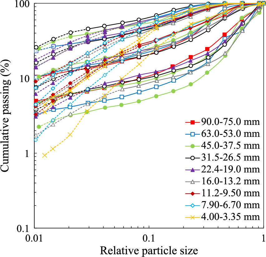
Progeny size distributions from testing gneiss particles from Santa Luzia quarry contained in different size ranges in drop weight testers (modified from Tavares and Neves, 2008).

One convenient method to deal with data such as those in Fig. 10 is to select particular markers on each curve. This is the so-called t₁₀ procedure originally proposed by Narayanan and Whiten (1988). As part of this procedure the percentage of material passing different 1/nth fractions of the initial particle size, called t_ns, are estimated from the cumulative size distribution, typically interpolated using cubic splines. Commonly used values of n are 2, 4, 10, 25, 50 and 75. With the aim of representing the progeny size distribution in greater detail, additional markers may also be used, including 1.2 and 1.5 (Carvalho et al., 2015; Ballantyne et al., 2017). In order to illustrate this, breakage data in Fig. 10 are presented in normalized form in Fig. 12, which shows that data for each n value follows well-defined trends as a function of t₁₀. The principle of the method is that, if the user has an estimate of the t₁₀ value of the size distribution, likely from an expression that relates the initial particle size and the specific impact energy, the entire size distribution can be reconstructed (Napier-Munn et al., 1996; Tavares, 2017).

Fig. 12

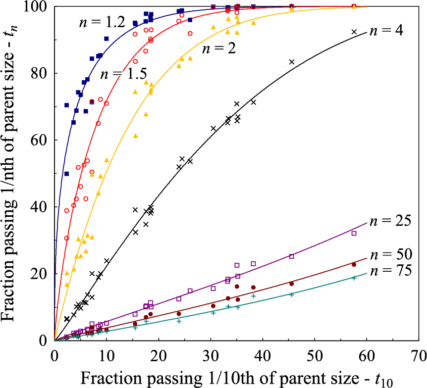
Progeny size distributions presented in the normalized t₁₀ versus t_n format for syenite from Vigné quarry (data from Fig. 10).

Several functional forms have been proposed over the years to describe cumulative progeny size distributions from drop weight tests, including the cubic splines (Narayanan and Whiten, 1988; Napier-Munn et al., 1996), the upper truncated Rosin-Rammler (King, 2001; Tavares, 2004) and combined exponential functions (Ballantyne et al., 2017). Given its ability to describe data with great flexibility, the incomplete beta function is used as part of the present model (Carvalho et al., 2015), given by   

$$t_n\left(t_{10}\right)=\frac{100}{{\int }_0^1{x}^{{\alpha }_n-1}{\left(1-x\right)}^{{\beta }_n-1}\hspace{0.17em}\text{d}x}{\int }_0^{t_{10}/100}{x}^{{\alpha }_n-1}{\left(1-x\right)}^{{\beta }_n-1}\hspace{0.17em}\text{d}x$$(16)

where the cumulative mass of the particles passing a screen (t_n) with relative size x is calculated by the given t₁₀ value of the distribution. In the model two parameters (α and β) must be fitted to each value of n selected. As such, with the seven n values (1.2, 1.5, 2, 4, 25, 50 and 75) a total of 14 parameters must be fitted from data, which is substantial.

Fig. 12 shows that data can be well described using Eqn. (16). The equation has also demonstrated to successfully fit the data for several other materials, as was also evident in previous publications (Barrios et al., 2011; Carvalho and Tavares, 2013; Carvalho et al., 2015). Unfortunately, given the lack of a proper physical description of fragmentation that would allow extrapolation of data, characterizing the response of a given material requires extensive testing over a range of stressing energies and sizes, which is a time-consuming task. Although it may be argued that each material has its well-defined breakage pattern, so that they will present different t₁₀ versus t_n relationships such as the one presented in Fig. 12 (Tavares and Neves, 2008), it is worthwhile to search for a mean distribution that would be able to describe data for a variety of materials with reasonable confidence.

As such, data from drop weight tests of a total of 40 materials have been gathered (Tavares and Chagas, 2021) and plotted in normalized axes as those in Fig. 12, with results being presented in Fig. 13 for selected values of n. A large scatter in the data appears, but it is also evident that data can be reasonably well represented using a single set of curves. The scatter in the graph in a logarithmic scale suggests the structure of the errors and the validity of the logarithmic objective function used in fitting the model parameters (Carvalho et al., 2015).

Fig. 13

Relationship between t₁₀ and selected t_ns for a variety of materials, with the exception of iron ores. Solid lines represent the fit to the incomplete beta function (data from Tavares and Chagas, 2021).

A more detailed examination of the data (Tavares and Chagas, 2021) allowed to conclude that the different types of materials (rocks, ores, cement clinkers and coals) did not appear particularly segregated in each of the plots in Fig. 13, which suggests the validity of the generalization proposed. The only exceptions were iron ores (Tavares and Chagas, 2021), which were not included in model fitting. Also, deviations were typically limited to the extremes of the size distributions, that is, either at the coarse (t_1.2 and t_1.5) or the fine (t₅₀ or t₇₅) end.

The list of parameters that resulted from fitting the data in Fig. 13 is presented in Table 2, covering the 40 materials (Tavares and Chagas, 2021). These parameters may be used as default in case of the absence of enough fragmentation data that would allow fitting of the various parameters in Eqn. (16) for a material of interest.

Table 2 Optimal parameters of the incomplete beta function (Eqn. 16) for 40 materials (Tavares and Chagas, 2021), without including iron ores.

n	αn	βn
1.2	0.448	10.508
1.5	0.706	7.913
2	0.959	5.780
4	1.105	2.619
25	0.981	0.524
50	0.956	0.339
75	0.934	0.255

Fig. 14 is obtained by plotting the various t_n values as a function of normalized fragment size for selected t₁₀ values using Eqn. (16) with parameters given in Table 2.

Fig. 14

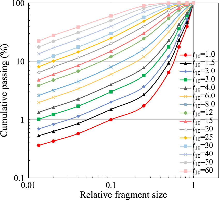
Calculated normalized size distributions using the incomplete beta function and parameters from Table 2 (Tavares and Chagas, 2021). Symbols represent the calculated t values for the different n markers, while lines are cubic spline fits (Eqn. 17) to these values.

Although not included in the present work (Cavalcanti et al., 2021), data from projecting particles against a target could also be well described using the incomplete beta function and parameters from Table 2.

The normalizable breakage function can then be obtained from Eqn. (16) using the ratio between the fragment size D_i and the parent particle size d_j, so that   

$$B_{ij}\hspace{0.17em}\left(t_{10}\right)=B\left(x,t_{10}\right)=\text{interp}\left(t_{10},x\right)$$(17)

where x = d_i/D_j.

As mentioned earlier in the section, there are instances in which the normalization approach proposed by the t₁₀ procedure is not valid below a given fragment size D*. This is the case of the so-called non-normalizable progeny size distributions, which appear typically when materials have a well-defined dimension in which discontinuities concentrate (Tavares, 2000). Indeed, non-normalizable breakage functions have occasionally been used with the population balance model equations for materials such as iron ores (Faria et al., 2019; Campos et al., 2019). Table 3 shows examples of materials whose breakage description required the non-normalizable part of the breakage distribution.

Table 3 Fragment sizes below which progeny size distributions are not normalizable for selected materials (Eqn. 18).

Material	Particle size – D* (mm)	η	Reference
Vermont marble	0.32	1.46	Tavares (1997)
Utah siltstone	0.15	0.59	Tavares (1997)
IOCC iron ore	0.35	1.83	Tavares (1997)
Pedra Sul granulite	0.17	0.64	Barrios et al. (2011)
Santa Luzia gneiss	0.80	0.80	Tavares and Neves (2008)

This behavior can be described in the form of a power-law relationship below a minimum normalization size D*,   

$$\begin{array}{l}{B}_{ij}=B\left(D_i,d_j\right)=B_{i-j}\hspace{0.17em}\text{for\hspace{0.17em}}{D}_i<D^{*}\\ B_{ij}=B\left(D_i,d_j\right){\left(\frac{D_i}{D^{*}}\right)}^{\eta }\hspace{0.17em}\text{for\hspace{0.17em}}{D}_i<D^{*}\end{array}$$(18)

which shows that the non-normalizable part of the distribution is attached to the fine end of the normalizable progeny size distribution obtained using the incomplete beta function (Eqn. 16). Values of the exponent η are shown in Table 3 for selected materials. It is worth comparing these to the average slope at fine sizes from the model for the 40 materials (Fig. 14), which varies from 0.53 at low t₁₀ values to 0.63 (Tavares and Chagas, 2021).

Adapting the present model to describe breakage of discrete particles in DEM has been carried out by different methods, depending on the shapes of particles. In the case of polyhedral particles (Tavares et al., 2020a) these have been used as part of the Voronoi tessellation scheme to create the appropriate fragment size distribution and are implemented in the commercial software Rocky DEM. On the other hand, in order to represent breakage of spherical particles in a DEM simulation, families of spherical progeny have been created for a variety of values of t₁₀ using a procedure described elsewhere (Tavares and Chagas, 2021). This later has been implemented in the commercial software Altair EDEM (Tavares et al., 2021).

The described normalization procedure only accounts partially for the effect of particle size. The additional effect of particle size associated to the increase in resistance to breakage as particle sizes reduce, as well as the effect of stressing energy, are described using expressions presented in detail in section 3.2. In addition to those, studies have shown that other variables, such as impact geometry (Tavares, 2007; Saeidi et al., 2016), stressing rate (Saeidi et al., 2017) and mode of stressing, if single or double impact (Tavares, 2007), are known to have an influence on breakage distribution. However, the lack of a proper understanding of their effect made it unfeasible to take them into account explicitly in the model.

At stressing energies that are insufficient to cause body breakage, particles will undergo surface breakage. Carvalho and Tavares (2011) proposed to describe it using the Gaudin-Schuhmann equation   

$$\begin{array}{l}{A}_{ij}=1\hspace{0.17em}\text{for\hspace{0.17em}}{d}_i\ge d_{\text{A}}\\ A_{ij}={\left(\frac{d_i}{d_{\text{A}}}\right)}^{\lambda }\hspace{0.17em}\text{for\hspace{0.17em}}{d}_i<d_{\text{A}}\end{array}$$(19)

where d_A is the top size of surface breakage products, which together with λ, must be fit from data. The variation of these as a function of parent particle size and stressing energy has not been studied in as much detail in the literature. From tumbling tests d_A has been found to vary typically from about 0.20 to 0.45 mm (Tavares and Neves, 2008; Carvalho and Tavares, 2011). This parameter will likely be strongly influenced by parent particle size, but the data are not yet comprehensive enough to characterize such dependence (Cavalcanti et al., 2021).

3.2 Effect of particle size and stressing energy on body breakage distribution

In the original t₁₀ method (Narayanan and Whiten, 1988; Napier-Munn et al., 1996), size-independent relationships between the stressing energy and the t₁₀ value were proposed. In the present model the relationship accounts simultaneously for the effects of stressing energy and particle size, this later incorporated in the median fracture energy of particles (Tavares, 2009),   

$$t_{10}=A\left[1-\text{exp}\left(-\frac{b^{\prime }e{E}_k}{E_{50\text{b}}}\right)\right]$$(20)

where A and b′ are model parameters fitted to experimental data, in which A corresponds to the maximum value of t₁₀ that can be achieved when breaking a material in a single stressing event, whereas E_50b is the median specific fracture energy of particles that underwent breakage. The higher the specific impact energy E_k in comparison to the specific fracture energy of the particles, the higher the value of t₁₀ and the finer the progeny size distribution. By using the median specific fracture energy of the particles that underwent breakage, Eqn. (20) is able to account for the particle size effect in breakage.

Data from a variety of materials have been fitted to Eqn. (20) and results are listed in Table 4. Values of parameter A, representing the maximum t₁₀ value achieved in a single stressing event, were found to vary between about 40 to 75, with typical values around 50 %. This demonstrates that a limiting maximum fineness can be achieved in a single stressing event on individual particles, regardless of the intensity of the stressing energy. The product of the parameters (A*b′), which corresponds to the derivative of Eqn. (20) at the origin, represents the amenability of the material to fragmentation. Since the toughness of the material is already captured in the value of E_50b, this product actually characterizes how effectively the stressing energy is used to create new fracture surfaces and fragments. Its values range from as low as 0.5 % to as high as 10 % (Table 4). As such, some grouping in respect to type of material has been observed (Tavares, 2000), in which materials with simple microstructures, such as individual minerals or crystals, present values below about 1 %, whereas most rocks and ores present values in the range from about 1 and 2 %. Values higher than 2 % have been observed for ores and rocks with poor intergranular bonding (Tavares, 2000), coals, as well as some porous materials, such as cement clinkers.

Table 4 Values of parameters A and b′ (Eqn. 20) for selected materials.

Mineral/ore/rock	Source	A	b′	A*b′	Reference
Apatite	Cantley, Canada	45.4	0.012	0.52	Tavares (2007)
Quartz	Karlsruhe, Germany	38.8	0.018	0.68	Tavares (2007)
Hematite	Québec, Canada	45.6	0.016	0.75	Tavares (2007)
Galena	Park Valley, Idaho	44.5	0.018	0.78	Tavares (2007)
Copper-gold ore	Australia	66.2	0.013	0.85	Tavares et al. (2020b)
Granulite	Embu, Brazil	62.6	0.014	0.90	Tavares and Neves (2008)
Limestone	Utah	54.5	0.018	0.96	Tavares (2007)
Syenite	Vigné quarry, Brazil	58.0	0.017	0.97	Tavares and Neves (2008)
Limestone	Ribeirão Branco, Brazil	46.6	0.022	1.03	—
Copper ore (K)	Bingham Canyon, Utah	44.8	0.026	1.18	Tavares (2007)
Copper ore	Cyprus Sierrita, Arizona	58.9	0.020	1.20	Tavares (2007)
Granulite	Pedra Sul, Brazil	47.5	0.027	1.27	Tavares and Neves (2008)
Iron ore	Conceição Mine, Brazil	44.2	0.029	1.27	Tavares and Carvalho (2011)
Basalt	Utah	52.0	0.025	1.31	Tavares (2007)
Titanium ore	Titania, Norway	51.0	0.027	1.37	Tavares (2007)
Gneiss	Santa Luzia, Brazil	59.7	0.025	1.50	Tavares and Neves (2008)
Limestone #1	Brazil	53.3	0.033	1.76	Barrios et al. (2011)
Cement Clinker A	CEMEX, Mexico	69.2	0.028	1.91	Tavares (2007)
Copper ore (S)	Sossego, Brazil	67.7	0.029	1.96	Barrios et al. (2011)
Limestone #2	Brazil	63.4	0.033	2.09	Carvalho and Tavares (2013)
Cement Clinker B	CEMEX, Mexico	60.5	0.044	2.64	Tavares (2007)
Gold ore	South Africa	44.1	0.060	2.65	Pauw and Maré (1988)
Iron ore	Brazil	60.4	0.051	3.08	Carvalho and Tavares (2013)
Coal	Candiota, Brazil	44.1	0.091	4.01	—
Marble	Vermont	76.3	0.079	6.04	Tavares (2007)
Iron ore	Newfoundland, Canada	65.4	0.158	10.3	Tavares (2007)

Typical results from fitting the model to data are presented in Fig. 15, which shows the good agreement between the two. In some cases, however, the scatter is larger when particles of several sizes are included in the fit, potentially a consequence of effects that are not accounted for in the model, such as variation in standard deviation of the distribution with particle size, impact velocity and particle shape. The direct connection in the model between the breakage probability and the fragment distribution, offered by the normalizing value of E_50b in Eqn. (20), is considered an important feature, which renders internal consistency in the model.

Fig. 15

t₁₀ as a function of impact energy for different particle size ranges of limestone #1.

Adapting the model given by Eqn. (20) to describe breakage of discrete particles results in the modified equation (Tavares et al., 2021)   

$$t_{10}^{\prime }=A\left[1-\text{exp}\left(-\frac{b^{\prime }ke{E}_k}{E}\right)\right]$$(21)

where k is a variable introduced because the mean and the median values of the distribution do not coincide (Tavares and Chagas, 2021). This expression has been used in association to discrete implementations of the model for the case of either spherical (Tavares and Chagas, 2020; Tavares et al., 2021) or polyhedral particles (Tavares et al., 2020a) in DEM.

4. Model implications

4.1 Primary body breakage function

In several mills and crushers, the breakage distribution function is widely used to describe the average size distribution from each stressing event inside the devices, playing a central role in traditional population balance models (Austin et al., 1984; King, 2001). In practice, rather than a true material property, it represents the result of model fitting, at best estimated on the basis of the size distribution from short grinding times (Austin et al., 1984).

For the case in which the particle is stressed with the minimum energy to produce body breakage, the resulting fragment distribution is called primary single-particle breakage function (Saeidi et al., 2016). In the few studies that attempted to measure directly this primary breakage distribution function of individual particles, Bourgeois (1993) estimated in about 2 % the value of t₁₀ for quartz particles under double impact (Saeidi et al., 2016), whereas the corresponding value was about 1 % for iron ore pellets subjected to single impact (Cavalcanti et al., 2021). Tavares (2009) then demonstrated, for a sample of limestone, that it did not vary after each repeated impact. The importance of this primary single-particle breakage function has been demonstrated by Saeidi et al. (2016), who showed that it was possible to predict the response of a material in a drop weight tester to higher impact energies on the basis of this primary breakage function, besides Eqn. (10) and empirical functions representing probability of selection of fragments to secondary breakage. This has also been demonstrated to be valid in DEM environment, where the size distribution from higher impact energies could be predicted using the breakage model in the case of polyhedral particles in Rocky DEM (Tavares et al., 2020a) and Altair EDEM (Tavares et al., 2021).

The present model allows estimating this primary breakage function by considering the case in which eE_k ≅ E in Eqn. (21), giving

  

$$t_{10}^{\prime }\cong A[1-\text{exp}(-b^{\prime })]$$(22)

Given the values of the constants A and b′ (Table 4) and since at such low impact energies the constant k in Eqn. (22) may be considered equal to about 0.95 (Tavares and Chagas, 2021), then the resulting t₁₀ values corresponding to primary breakage range from as low as 0.5 to, exceptionally, higher than 5 %. As such, from comparison with the experimental measurements by Bourgeois (1993) and Cavalcanti et al. (2021), values estimated using Eqn. (22) are likely an underestimation of the actual value. Nevertheless, they may be considered generally valid, given the challenge in estimating directly the primary body breakage function.

With the aim of illustrating the variations encountered for different materials, Fig. 16 compares primary body breakage distribution functions for selected materials estimated using this approach. It shows the variations in shape and position of the primary fragment size distributions, representing differences in fragmentation pattern, with the single-phase materials (minerals) generating less fines than rocks/ores (Tavares, 2000).

Fig. 16

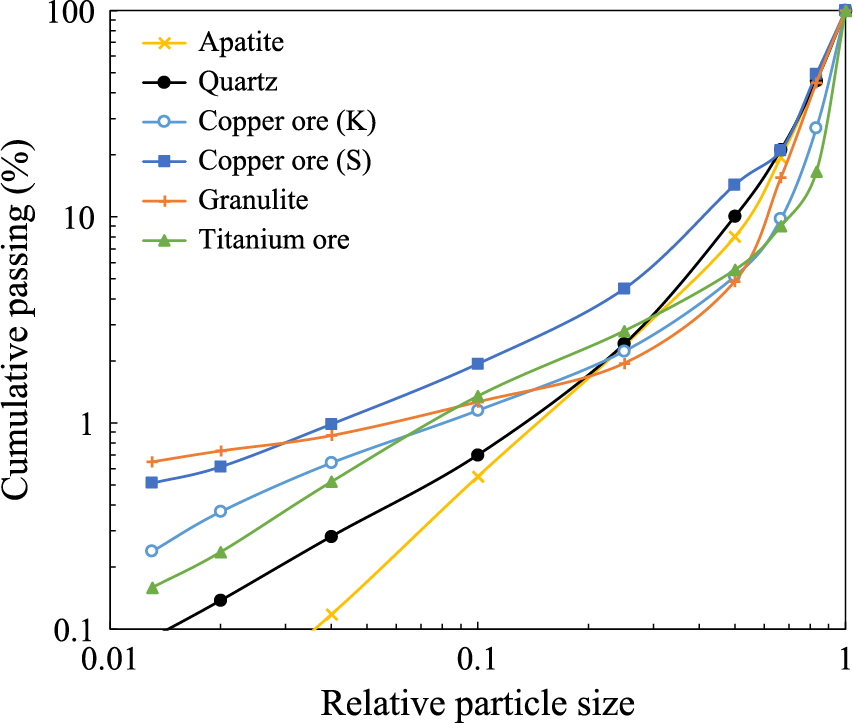
Primary breakage functions for selected materials, obtained by fitting single-particle breakage data to the incomplete beta function for t₁₀ given by Eqn. (22).

4.2 Predicting the outcome of a single stressing event

Arguably, the simplest demonstration of the application of a breakage model is to predict the outcome of a single impact on individual particles, such as in drop weight tester (Napier-Munn et al., 1996; Tavares, 2007). The outcome of this single impact event, considering both body and surface breakage, may be described by the mass balance given by (Tavares and Carvalho, 2011)   

$$\begin{array}{l}{w}_i^{*}=w_i\left[1-P_i\left(e{E}_k\right)\right]\hspace{0.17em}\left[1-{\xi }_i\left(e{E}_k\right)\right]\\ +\sum _{j=1}^i{w}_j\hspace{0.17em}\left\{P_j\left(e{E}_k\right)b_{ij}\left(e{E}_k\right)+{\xi }_i\left(e{E}_k\right)\left[1-P_j\left(e{E}_k\right)\right]\hspace{0.17em}{a}_i\right\}\end{array}$$(23)

where $w_i^{*}$ and w_i are the weight fractions of the material contained in size class i after and before the impact event, respectively. ξ_i is the fractional generation of surface breakage products, a_ij is the surface breakage distribution function and b_ij is the energy-specific body breakage distribution function. The term [1 − P_i(eE_k)][1 − ξ_i(eE_k)] on the right-hand side of Eqn. (23) represents the mass fraction of material that did not suffer body breakage during the stressing event and remained in the original size, whereas the term ${\mathrm{\Sigma }}_{j=1}^i{w}_j\hspace{0.17em}\left[P_j\left(e{E}_k\right)b_{ij}\left(e{E}_k\right)\right]$ represents the proportion of material from size classes i and coarser that suffered body breakage and generated fragments reported to size class i. The term ${\mathrm{\Sigma }}_{j=1}^i{w}_j\hspace{0.17em}\left\{{\xi }_i\left(e{E}_k\right)\left[1-P_j\left(e{E}_k\right)\right]\hspace{0.17em}{a}_i\right\}$ gives the cumulative proportion of surface breakage products that reports to size class i. P_i(eE_k) is the probability that a particle contained in size class i will suffer body breakage when it captures energy eE_k from a collision event.

When varying the specific impact energy applied to a batch of particles, breakage can transition from no body breakage at very low impact energies, where all particles undergo only surface breakage, to body breakage of all particles at high impact energies. In between these are impact energies in which a fraction of the particles underwent body breakage, whereas the remainder only suffered surface breakage. This is illustrated in Fig. 17 for particles of Pedra Sul granulite. In the figure, stressing energies above 360 J/kg were able to produce body breakage in the first impact on all particles, whereas those at 9 J/kg produced only surface breakage. For stressing energies between these, only a fraction of the particles underwent body breakage, resulting in size distributions that represent the transition between surface and body breakage. Unfortunately, validation data are available only for the higher impact energies, since at the lower impact energies the small amount of surface breakage products makes collection of accurate data a challenging task.

Fig. 17

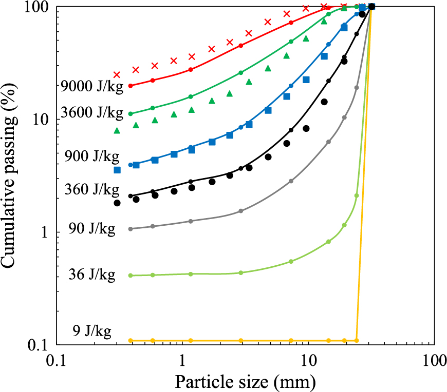
Progeny size distributions from impact of 31.5–26.5 mm granulite (Pedra Sul) particles in a drop weight tester at variable specific impact energies. Large symbols represent experiments and lines and small circles model predictions. σ = 0.90, κ = 4 × 10⁻⁴ kg/mmJ. Other parameters given in Tables 1 and 4.

5. Discussion

5.1 Breakage testing and model fitting

The breakage model contains a variety of parameters that must be fitted on the basis of experiments. Although some parameters, in particular those related to the fragment size distribution, may be assumed as default, since their variation for different materials may be relatively limited (section 3.1), experiments are required to estimate the several remaining ones. The originally proposed and most direct approach to estimate parameters from the model was based on the use of the impact load cell device (Tavares, 2007). It is an instrumented drop weight tester in which the minimum energy required for primary fracture (Tavares and King, 1998) as well as the net energy absorbed (Tavares, 1999) may be estimated for each individual particle. Besides that, repeated impact tests have then been used to estimate the damage accumulation parameter (section 2.3), whereas the fragment size distributions from different impact energies served as the basis to fitting the parameters in the model described in 3.2. Slow compression tests can also be used to estimate the fracture energy distribution of particles. Data from non-instrumented devices can also be used to estimate the parameters in several of the model equations. For instance, the breakage probability distributions may be estimated from either standard drop weight tests (Baumgardt et al., 1975) or tests in which particles are projected against a target (Dan and Schubert, 1990; Cavalcanti et al., 2021). These later are particularly relevant when modeling with the aim of simulating material degradation during handling.

Although the detailed analysis of the experimental procedures and devices used to fit parameters in the breakage model is beyond the scope of the present work and is well covered in other publications (Tavares and King, 1998; Tavares, 2007; Rozenblat et al., 2012; Ribas et al., 2014; Bonfils, 2017), it is worthwhile to highlight some important issues related to the tests. Indeed, one key challenge when estimating the fracture energy of individual particles using Eqn. (5) is the identification of primary fracture. This primary fracture or primary body breakage point is given by the condition in which the force suddenly drops, given the inability of the particle to continue transmitting stresses. Such condition is relatively straightforward to identify in some cases, such as in Fig. 18a, which is often found from testing regularly-shaped brittle particles. In these cases separation of newly created fracture surfaces is rapid, resulting from propagation of a major crack through the entire particle, facilitating the identification of the fracture point, given the sudden drop in load. In other cases, however, identifying the instant of fracture can be far more challenging and amenable to subjective judgement. A few examples of such cases are also illustrated in Fig. 18. Fig. 18b shows the case in which the particle suffered chipping at approximately 100 ms, but that primary breakage is still relatively straightforward to identify. This response is often found while testing highly irregularly-shaped particles, in which a small fraction of their volume becomes subjected to concentration of tensile stresses early in the test, causing the appearance of such superficial cracks. Yet in other cases either multiple peaks appear (Fig. 18c) or no clear fracture point may be identified (Fig. 18d), requiring some subjectivity in identifying the fracture load. Challenges such as these appear in association to testing more deformable and/or less brittle materials. This can be associated to cases in which either a single crack or several cracks grow sub-critically, being responsible for not such a clear reduction in load at primary fracture. However, since no relative motion of the fragments occur, due to the limited brittleness of the particle, the fragments continue to be able to sustain load, preventing a drop in load-bearing ability of the particle and, therefore, identification of the instant of primary breakage. Techniques that can be used to assist in interpreting these results will be analyzed in greater detail in a future publication.

Fig. 18

Typical force-time profiles from breakage of single particles of 12.5–9.0 mm iron ore pellets and their fragments in an impact load cell device. Arrows depict presumed primary breakage point.

A few useful guidelines when conducting experiments with the aim of estimating the distribution of particle fracture energies are:

• •   Particles should be contained in very narrow size ranges, ideally resulting from sieving following a $\sqrt[4]{2}$ series;
• •   Particle selection for the test should be conducted randomly, so as to guarantee that each lot tested has approximately the same average weight;
• •   Sample preparation should be carried out carefully, so as to avoid the use of crushing processes that may be responsible for generating flaky material, such as roll crushing (Gupta, 2016). Ideally either no crushing or the adoption of the size reduction process that is meant to be used in the targeted industrial operation should be preferred. Also, size reduction processes which are known to induce cracks in particles, sub as high-pressure roll grinding (Tavares, 2005), should also be avoided, whenever possible, in this task;
• •   Differences in particle shapes introduce variability in the distribution (Tavares, 2007; Lois-Morales et al., 2020). One possibility to deal with this is to segregate particles contained within the $\sqrt[4]{2}$ series according to mass and test separately. If that approach is not used, particles should be randomly selected and the size of the tested lot increased accordingly with the variability;
• •   The number of particles tested in each size range must be at least 30, but should increase as the variability of particle composition and shape in the sample also increases, so that 50 or 100 are typically optimal;
• •   In the case of tests in impact load cell devices, it is advisable to select an average specific impact energy for the test (Eqn. 2) that is just high enough to break the toughest particle in the lot. The use of specific impact energies that are much higher than those must be avoided, in particular in the case of testing less brittle materials, since they can lead to greater difficulty in identifying properly the load responsible for primary fracture (Fig. 18d).

While particles in the size range from 100 mm (Fandrich et al., 1998; Tavares, 2007) down to 0.25 mm (Tavares and Cerqueira, 2007) have been tested in impact load cell devices, the greatest challenge lies in measuring fracture energies of particles contained in the lower range and even finer sizes, given the tedious nature of testing single particles and the limitation in the resolution of the devices. Some researchers have demonstrated the potential of measuring the strength and fracture energies of fine particles in special devices (Steier and Schönert, 1972; Yashima et al., 1979; Sikong et al., 1990; Antonyuk et al., 2005; Nguyen et al., 2009; Yan et al., 2009). Ribas et al. (2014) showed the potential of using a commercially-available micro compression tester to measure the fracture energy distributions of single particles in the 45–37 μm size range, whereas Campos et al. (2021) recently applied it to test iron ore particles contained in the range of 45 to 150 μm, with good results. Nevertheless, due to the challenge in measuring breakage characteristics of single particles down to such fine sizes, some indirect estimation approaches have been proposed. Barrios et al. (2011) proposed testing particles as fine as 150 μm contained in monolayer particle beds, combining them to data from single-particle breakage tests at coarser sizes, and estimating the breakage parameters from back-calculation, with reasonable success. More recently, Tavares et al. (2020b) proposed combining measurements of particle fracture energies of particles at relatively coarse sizes to data from impact tests using a rotary breakage tester. This allowed estimating selected material breakage parameters of a copper-gold ore down to 350 μm (Tavares et al., 2020b).

Yet another alternative to estimate breakage parameters in Eqn. (10) is to back-calculate them from batch grinding tests, assuming that predictions using the UFRJ mechanistic mill model (Tavares and Carvalho, 2009; Carvalho and Tavares, 2013) are strictly accurate. This approach has been used to estimate breakage parameters of an iron ore from batch milling data (Carvalho et al., 2021) as well as of limestone to stirred milling data (Oliveira et al., 2020). In these cases, the parameters from Eqns. (7), (12), (16) and (20) were taken from similar ores.

Evidently, errors can appear in estimates from back-calculation, since they rely on the validity of the various assumptions. In the particular case when only batch grinding results are used, errors may be associated to the fact that any limitation in the mill model in describing the phenomenon would inevitably contaminate the estimates of material breakage parameters, partially contradicting the very approach of the advanced models in fully decoupling material from process. In addition to that, this approach also requires that some parameters be taken from similar materials, which also involves a potential source of bias, since each material is intrinsically unique in regard to breakage response.

As discussed in section 3.3, more effort should be dedicated to modeling the primary breakage function from single-particle breakage, given its central role in the application of the model in particular to discrete systems in DEM. One device that could be useful in this task is the rigidly-mounted roller mill, which crushes particles nearly individually between rigidly-mounted rollers with carefully controlled gaps (Böttcher et al., 2021). In spite of challenges in measuring the energy required to break particles contained in the finest sizes studied (45 μm), it provided good estimates of the size distribution of particles under stressing conditions that approach the minimum required for fracture (Campos et al., 2021).

5.2 Model applications

The breakage model described has been used either in complete form or in parts in simulating different systems of interest using a variety of approaches. In its discrete form it has been embedded in DEM as part of different particle replacement schemes. Initially, a cutdown version of the model, which did not incorporate description of weakening by repeated impacts (section 2.4), was implemented in EDEM (Jiménez-Herrera et al., 2018; Barrios et al., 2020), demonstrating some ability to describe breakage in both confined and unconfined particle beds. A more complete version of the model, incorporating a new stochastic description of particle replacement (Tavares and Chagas, 2021) was implemented in an updated version of EDEM (Tavares et al., 2021), demonstrating very good ability to predict unconfined breakage of particle beds. Both approaches were based on spherical particle replacement, which has the advantage of computational efficiency. This later implementation also incorporated description of the unresolved fines, which were added upon completion of the simulation to the size distribution given by the resolved spheres. The more complete version of the model has also been implemented in the commercial software package Rocky DEM (Tavares et al., 2020a). Such implementation, based on breakage of polyhedral particles, provided very good predictions of breakage in unconfined particle beds (Tavares et al., 2020a) and cone crushing (André and Tavares, 2020).

The breakage model has also been widely used as part of advanced models of crushers and mills. For instance, Austin (2004a; 2004b) used the damage model from section 2.4 in a phenomenological model of high-speed hammer milling. The full version of the breakage model has been used to predict degradation during handling of materials (Tavares and Carvalho, 2011). It has also been used, coupled to DEM, to model crushing in a vertical shaft impact crusher (Cunha et al., 2014), as well as of degradation of recycled aggregate in a high-shear mixer (Moreno-Juez et al., 2021). The modeling approach has also been used to predict degradation of iron ore pellets during handling using slightly customized mathematical expressions (Cavalcanti et al., 2019; 2021; Tavares et al., 2018). The widest use of the model has been in association to a microscale population balance formulation, called UFRJ model, to describe grinding in media mills, including ball mills (Tavares and Carvalho, 2009; Carvalho and Tavares, 2013), semi-autogenous mills (Carvalho and Tavares, 2011) and stirred mills (Oliveira et al., 2020; 2021). A version of the ball mill model of continuous milling with some simplifications is available in the state-of-the-art mining and mineral processing plant simulator IES (Integrated Extraction Simulator).

6. Summary and conclusions

A practical model describing breakage of single particles has been proposed over the last 25 years. It discriminates body and surface breakage, accounting for the body breakage probability through the upper-truncated lognormal distribution. It is able to predict breakage by repeated impacts owing to a model describing weakening based on continuum damage mechanics. Body-breakage progeny size distribution is described using the incomplete beta function, which also considers the exceptional cases in which the material exhibits non-normalizable breakage response. With an empirical expression that describes the stressing energy and size-dependent breakage intensity, it can predict the size distribution of fragments from any stressing event.

This breakage model has been implemented and is now an integral part of particle replacement schemes embedded in commercial DEM software (Rocky DEM and Altair EDEM), through which it may be used to simulate a number of industrial processes of interest. It has also been incorporated in microscale population balance models describing several mill types, namely ball mills, stirred mills, autogenous and semi-autogenous, being even available (ball mill model) in the plant simulator IES.

While being able to account for several important variables that influence particle breakage, challenges are identified in application and fitting of the model parameters for particular applications. Being a single-particle-based model, challenges exist in estimating breakage parameters for fine particles. Establishing the validity of novel testing devices as well as of back-calculation approaches, is an important task. Further, modifications in the model in order to make it applicable to describe breakage of non-brittle materials (Tavares and Almeida, 2020) is another worthwhile task for advancing model applicability. Finally, models describing surface breakage, which are particularly relevant in predicting mechanical degradation during handling, require more attention, since they are still at a comparatively earlier stage of development and validation.

Acknowledgements

The author would like to thank the financial support from the Brazilian agencies CNPq (grant number 310293/2017-0) and FAPERJ (grant number E-26/202.574/2019), as well as the team of researchers in his group and outside collaborators for their contributions throughout the development of this work.

References

•  André  F.P.,  Tavares  L.M., Simulating a laboratory-scale cone crusher in DEM using polyhedral particles, Powder Technology, 372 (2020) 362–371. DOI: 10.1016/j.powtec.2020.06.016
•  Angulo  S.C.,  Silva  N.V.,  Lange  D.A.,  Tavares  L.M., Probability distributions of mechanical properties of natural aggregates using a simple method, Construction and Building Materials, 233 (2020) 117269. DOI: 10.1016/j.conbuildmat.2019.117269
•  Antonyuk  S.,  Tomas  J.,  Heinrich  S.,  Mörl  L., Breakage behaviour of spherical granulates by compression, Chemical Engineering Science, 60 (2005) 4031–4044. DOI: 10.1016/j.ces.2005.02.038
•  Arbiter  N.,  Harris  C.C.,  Stamboltzis  G.A., Single fracture of brittle spheres, Transactions of the SME/AIME, 244 (1969) 118–133.
•  Austin  L.G., A preliminary simulation model for fine grinding in high speed hammer mills, Powder Technology, 143–144 (2004a) 240–252. DOI: 10.1016/j.powtec.2004.04.017
•  Austin  L.G., The effect of damage on breakage kinetics, Powder Technology, 143–144 (2004b) 151–159. DOI: 10.1016/j.powtec.2004.04.048
•  Austin  L.G.,  Klimpel  R.R.,  Luckie  P.T., Process Engineering of Size Reduction: Ball Milling, Society of Mining Engineers of the AIME, 1984, ISBN: 9780895204219.
•  Ballantyne  G.R.,  Bonfils  B.,  Powell  M.S., Evolution of impact breakage characterisation: re-defining t-family relationship, International Journal of Mineral Processing, 168 (2017) 126–135. DOI: 10.1016/j.minpro.2017.10.001
•  Barrios  G.K.P.,  de Carvalho  R.M.,  Tavares  L.M., Extending breakage characterisation to fine sizes by impact on particle beds, Mineral Processing and Extractive Metallurgy, 120 (2011) 37–44. DOI: 10.1179/1743285510y.0000000002
•  Barrios  G.K.P.,  Jiménez-Herrera  N.,  Tavares  L.M., Simulation of particle bed breakage by slow compression and impact using a DEM particle replacement model, Advanced Powder Technology, 31 (2020) 2749–2758. DOI: 10.1016/j.apt.2020.05.011
•  Baumgardt  S.,  Buss  B.,  May  P.,  Schubert  H., On the comparison of results in single grain crushing under different kinds of load, Proceedings of the 11th International Mineral Processing Congress, Cagliari, 1975, pp. 3–32.
•  Becker  M.,  Kwade  A.,  Schwedes  J., Stress intensity in stirred media mills and its effect on specific energy requirement, International Journal of Mineral Processing, 61 (2001) 189–208. DOI: 10.1016/s0301-7516(00)00037-5
•  Bergstrom  B.H.,  Sollenberger  C.L.,  Mitchell Jr.  W. , Energy aspects of single particle crushing, Transactions of the AIME, 220 (1961) 367–372.
•  Boechat  F.O.,  de Carvalho  R.M.,  Tavares  L.M., Simulation of mechanical degradation of iron ore pellets in a direct reduction furnace, KONA Powder and Particle Journal, 35 (2018) 216–225. DOI: 10.14356/kona.2018009
•  Bond  F.C., Crushing tests by pressure and impact, Transactions of the AIME, 169 (1947) 58–66.
•  Bonfils  B., Quantifying of impact breakage of cylindrical rock particles on an impact load cell, International Journal of Mineral Processing, 161 (2017) 1–6. DOI: 10.1016/j.minpro.2017.02.005
•  Bonfils  B.,  Ballantyne  G.R.,  Powell  M.S., Developments in incremental rock breakage testing methodologies and modelling, International Journal of Mineral Processing, 152 (2016) 16–25. DOI: 10.1016/j.minpro.2016.04.010
•  Böttcher  A.-C.,  Thon  C.,  Fragnière  G.,  Chagas  A.,  Schilde  C.,  Kwade  A., Rigidly-mounted roll mill as breakage tester for characterizing fine particle breakage, Powder Technology, 383 (2021) 554–563. DOI: 10.1016/j.powtec.2021.01.055
•  Bourgeois  F.S., Single-particle fracture as a basis for microscale modeling of comminution processes, Ph.D. thesis, The University of Utah, 1993. https://utah-primoprod.hosted.exlibrisgroup.com/permalink/f/dtufc4/UUU_ALMA21242038230002001
•  Capece  M.,  Bilgili  E.,  Davé  R.N., Formulation of a physically motivated specific breakage rate parameter for ball milling via the discrete element method, AIChE Journal, 60 (2014) 2404–2415. DOI: 10.1002/aic.14451
•  Campos  T.M.,  Bueno  G.,  Barrios  G.K.P.,  Tavares  L.M., Pressing iron ore concentrate in a pilot-scale HPGR. Part 1: experimental results, Minerals Engineering, 140 (2019) 105875. DOI: 10.1016/j.mineng.2019.105875
•  Campos  T.M.,  Bueno  G.,  Rodriguez  V.A.,  Böttcher  A.-C.,  Kwade  A.,  Mayerhofer  F.,  Tavares  L.M., Relationships between particle breakage characteristics and comminution response of fine iron ore concentrates, Minerals Engineering, 164 (2021) 106818. DOI: 10.1016/j.mineng.2021.106818
•  Carvalho  R.M.,  Campos  T.M.,  Faria  P.M.,  Tavares  L.M., Mechanistic modeling and simulation of grinding iron ore pellet feed in pilot and industrial-scale ball mills, Powder Technology, 392 (2021) 489–502. DOI: 10.1016/j.powtec.2021.07.030
•  Carvalho  R.M.,  Secchi  A.R.,  Tavares  L.M., A new breakage function model and optimization procedure for mechanistic comminution models, Proceedings of the 14th European Symposium on Comminution and Classification, Gothenburg, 2015, pp. 42–45.
•  Carvalho  R.M.,  Tavares  L.M., Leaping forward in SAG and AG mill simulation using a mechanistic model framework, Proceedings of the International Autogenous Grinding, Semi-Autogenous Grinding and High-Pressure Roll Technology Conference, Vancouver, 2011, pp. 1–26.
•  Carvalho  R.M.,  Tavares  L.M., Predicting the effect of operating and design variables on breakage rates using the mechanistic ball mill model, Minerals Engineering, 43–44 (2013) 91–101. DOI: 10.1016/j.mineng.2012.09.008
•  Cavalcanti  P.P.,  de Carvalho  R.M.,  das Chagas  A.S.,  da Silveira  M.W.,  Tavares  L.M., Surface breakage of fired iron ore pellets by impact, Powder Technology, 342 (2019) 735–743. DOI: 10.1016/j.powtec.2018.10.044
•  Cavalcanti  P.P.S.,  Petit  H.A.,  Thomazini  A.D.,  de Carvalho  R.M.,  Tavares  L.M., Modeling of degradation by impact of individual iron ore pellets, Powder Technology, 378 (2021) 795–807. DOI: 10.1016/j.powtec.2020.10.037
•  Cavalcanti  P.P.,  Tavares  L.M., Statistical analysis of fracture characteristics of industrial iron ore pellets, Powder Technology, 325 (2018) 659–668. DOI: 10.1016/j.powtec.2017.11.062
•  Cavalcanti  P.P.,  Tavares  L.M., Static and dynamic compressive loading of fired iron ore pellets, Powder Technology, 354 (2019) 281–288. DOI: 10.1016/j.powtec.2019.06.006
•  Cunha  E.R.,  Carvalho  R.M.,  Tavares  L.M., A predictive model of the Vertical Shaft Impact (VSI) crusher, Proceedings of the 9th International Comminution Symposium, Cape Town, 2014, 2014, v. 1. p. 1–13.
•  Dan  C.C.,  Schubert  H., Breakage probability, progeny size distribution and energy utilization of comminution by impact, Aufbereitungs-Technik, 31 (1990) 241–247.
•  Datta  A.,  Rajamani  R.K., A direct approach of modeling batch grinding in ball mills using population balance principles and impact energy distribution, International Journal of Mineral Processing, 64 (2002) 181–200. DOI: 10.1016/s0301-7516(01)00044-8
•  Fandrich  R.G.,  Clout  J.M.F.,  Bourgeois  F.S., The CSIRO Hopkinson bar facility for large diameter particle breakage, Minerals Engineering, 11 (1998) 861–869. DOI: 10.1016/s0892-6875(98)00073-9
•  Faria  P.M.C.,  Rajamani  R.K.,  Tavares  L.M., Optimization of solids concentration in iron ore ball milling through modeling and simulation, Minerals, 9 (2019) 366. DOI: 10.3390/min9060366
•  Ghadiri  M.,  Zhang  Z., Impact attrition of particulate solids. Part 1: a theoretical model of chipping, Chemical Engineering Science, 57 (2002) 3659–3669. DOI: 10.1016/s0009-2509(02)00240-3
•  Gupta  V.K., Determination of the specific breakage rate parameters using the top-size-fraction method: preparation of the feed charge and design of experiments, Advanced Powder Technology, 27 (2016) 1710–1718. DOI: 10.1016/j.apt.2016.06.002.
•  Jiménez-Herrera  N.,  Barrios  G.K.P.,  Tavares  L.M., Comparison of breakage models in DEM in simulating impact on particle beds, Advanced Powder Technology, 29 (2018) 692–706. DOI: 10.1016/j.apt.2017.12.006
•  Kachanov  L.M., Time of the rupture process under creep conditions (in Russian), Izy Akad. Nank SSR Otd Tech Nauk, 8 (1958) 26–31.
•  King  R.P., Modeling and Simulation of Mineral Processing Systems, 1st edition, Butterworth-Heinemann, London, 2001, ISBN: 978-0-08-051184-9.
•  King  R.P.,  Bourgeois  F.S., A new conceptual model for ball milling, Proceedings of the 18th International Mineral Processing Congress, Sydney, 1993, pp. 81–86.
•  Krogh  S.R., Crushing characteristics, Powder Technology, 27 (1980) 171–181. DOI: 10.1016/0032-5910(80)85019-4
•  Lois-Morales  P.,  Evans  C.,  Bonfils  B.,  Weatherley  D., The impact load cell as a tool to link comminution properties to geomechanical properties of rocks, Minerals Engineering, 148 (2020) 106210. DOI: 10.1016/j.mineng.2020.106210
•  Mishra  B.K.,  Rajamani  R.K., The discrete element method for the simulation of ball mills, Applied Mathematical Modelling, 16 (1992) 598–604. DOI: 10.1016/0307-904x(92)90035-2
•  Moreno-Juez  J.,  Tavares  L.M.,  Artoni  R.,  de Carvalho  R.M.,  da Cunha  E.R.,  Cazacliu  B., Simulation of the Attrition of Recycled Concrete Aggregates during Concrete Mixing, Materials, 14 (2021) 3007. DOI: 10.3390/ma14113007
•  Morrell  S., An alternative energy–size relationship to that proposed by Bond for the design and optimisation of grinding circuits, International Journal of Mineral Processing, 74 (2004) 133–141. DOI: 10.1016/j.minpro.2003.10.002
•  Morrison  R.D.,  Cleary  P.W., Using DEM to model ore breakage within a pilot scale SAG mill, Minerals Engineering, 17 (2004) 1117–1124. DOI: 10.1016/j.mineng.2004.06.016
•  Morrison  R.D.,  Shi  F.,  Whyte  R., Modelling of incremental rock breakage by impact – for use in DEM models, Minerals Engineering, 20 (2007) 303–309. DOI: 10.1016/j.mineng.2006.10.015
•  Napier-Munn  T.J., Mineral Comminution Circuits: Their Operation and Optimisation, Julius Kruttschnitt Mineral Research Centre, 1996, ISBN: 9780646288611.
•  Narayanan  S.S., Determination of comminution characteristics from single particle breakage tests and its application to ball mill scale-up, Transactions of the Institution of Mining and Metallurgy C, 97 (1988) 115–124.
•  Nguyen  V.B.,  Wang  C.X.,  Thomas  C.R.,  Zhang  Z., Mechanical properties of single alginate microspheres determined by microcompression and finite element modelling, Chemical Engineering Science, 64 (2009) 821–829. DOI: 10.1016/j.ces.2008.10.050
•  Oliveira  A.L.R.,  de Carvalho  R.M.,  Tavares  L.M., Predicting the effect of operating and design variables in grinding in a vertical stirred mill using a mechanistic mill model, Powder Technology, 387 (2021) 560–574. DOI: 10.1016/j.powtec.2021.04.057
•  Oliveira  A.L.R.,  Rodriguez  V.A.,  de Carvalho  R.M.,  Powell  M.S.,  Tavares  L.M., Mechanistic modeling and simulation of a batch vertical stirred mill, Minerals Engineering, 156 (2020) 106487. DOI: 10.1016/j.mineng.2020.106487
•  Ouchterlony  F.,  Sanchidrián  J.A., The Fragmentation-energy fan concept and the Swebrec function in modeling drop weight testing, Rock Mechanics and Rock Engineering, 51 (2018) 3129–3156. DOI: 10.1007/s00603-018-1458-5
•  Pauw  O.G.,  Maré  M.S., The determination of optimum impact-breakage routes for an ore, Powder Technology, 54 (1988) 3–13. DOI: 10.1016/0032-5910(88)80043-3
•  Piret  E.L., Fundamental aspects of grinding, Chemical Engineering Progress, 49 (1953) 56–63.
•  Powell  M.S.,  Hilden  M.,  Ballantyne  G.,  Liu  L.X.,  Tavares  L.M., The appropriate, and inappropriate, application of the JKMRC t10 relationship, Proceedings of the 27th International Mineral Processing Congress, Santiago, Gecamin, 2014, v. 1, pp. 1–13.
•  Ribas  L.,  Cordeiro  G.C.,  Toledo Filho  R.D.,  Tavares  L.M., Measuring the strength of irregularly-shaped fine particles in a microcompression tester, Minerals Engineering, 65 (2014) 149–155. DOI: 10.1016/j.mineng.2014.05.021
•  Rodnianski  V.,  Levy  A.,  Kalman  H., A new method for simulation of comminution process in jet mills, Powder Technology, 343 (2019) 867–879. DOI: 10.1016/j.powtec.2018.11.021
•  Rozenblat  Y.,  Portnikov  D.,  Levy  A.,  Kalman  H.,  Aman  S.,  Tomas  J., Strength distribution of particles under compression, Powder Technology, 208 (2011) 215–224. DOI: 10.1016/j.powtec.2010.12.023
•  Rozenblat  Y.,  Grant  E.,  Levy  A.,  Kalman  H.,  Tomas  J., Selection and breakage functions of particles under impact loads, Chemical Engineering Science, 71 (2012) 56–66. DOI: 10.1016/j.ces.2011.12.012
•  Rumpf  H., Physical aspects of comminution and new formulation of a law of comminution, Powder Technology, 7 (1973) 145–159. DOI: 10.1016/0032-5910(73)80021-x
•  Saeidi  F.,  Tavares  L.M.,  Yahyaei  M.,  Powell  M., A phenomenological model of single particle breakage as a multi-stage process, Minerals Engineering, 98 (2016) 90–100. DOI: 10.1016/j.mineng.2016.07.006
•  Saeidi  F.,  Yahyaei  M.,  Powell  M.,  Tavares  L.M., Investigating the effect of applied strain rate in a single breakage event, Minerals Engineering, 100 (2017) 211–222. DOI: 10.1016/j.mineng.2016.09.010
•  Salman  A.D.,  Biggs  C.A.,  Fu  J.,  Angyal  I.,  Szabó  M.,  Hounslow  M.J., An experimental investigation of particle fragmentation using single particle impact studies, Powder Technology, 128 (2002) 36–46. DOI: 10.1016/s0032-5910(02)00151-1
•  Salman  A.D.,  Fu  J.,  Gorham  D.A.,  Hounslow  M.J., Impact breakage of fertiliser granules, Powder Technology, 130 (2003) 359–366. DOI: 10.1016/s0032-5910(02)00237-1
•  Schönert  K., Role of fracture physics in understanding comminution phenomena, Transactions of the SME/AIME, 252 (1972) 21–26.
•  Schönert  K., Aspects of physics of breakage relevant to comminution, Proceedings of the 4th Tewksbury Symposium, Melbourne, 1979, pp. 3.1–3.9.
•  Schönert  K., Advances in comminution fundamentals and impacts on technology, Aufbereitungs-Technik, 32 (1991) 487–494.
•  Schubert  H., On the microprocesses of comminution. Aufbereitungs–Technik, 5 (1987) 237–246.
•  Sikong  L.,  Hashimoto  H.,  Yashima  S., Breakage behavior of fine particles of brittle minerals and coals, Powder Technology, 61 (1990) 51–57. DOI: 10.1016/0032-5910(90)80065-7
•  Steier  K.,  Schönert  K., Verformung und Bruchphanomene unter druckbeanspruchung von sehr kleinen kornern aus Kalkstein, Quarz und Polystyprol, Dechema-Monographien, 69 (1972) 167–192.
•  Tavares  L.M., Microscale investigation of particle breakage applied to the study of thermal and mechanical predamage, Ph.D. thesis, University of Utah, 1997. https://utah-primoprod.hosted.exlibrisgroup.com/permalink/f/1g0gstr/TN_cdi_proquest_journals_304394788
•  Tavares  L.M., Energy absorbed in breakage of single particles in drop weight testing, Minerals Engineering, 12 (1999) 43–50. DOI: 10.1016/s0892-6875(98)00118-6
•  Tavares  L.M., Role of particle microstructure in comminution, Proceedings of the 21st International Mineral Processing Congress, Rome, Elsevier, 2000, Vol. C, pp. C4-99–C4-106.
•  Tavares  L.M., Optimum routes for particle breakage by impact, Powder Technology, 142 (2004) 81–91. DOI: 10.1016/j.powtec.2004.03.014
•  Tavares  L.M., Particle weakening in high-pressure roll grinding, Minerals Engineering, 18 (2005) 651–657. DOI: 10.1016/j.mineng.2004.10.012
•  Tavares  L.M., Breakage of single particles: quasi-static. In:  A.D.  Salman,  M.  Ghadiri,  M.J.  Hounslow (Eds.), Handbook of Particle Breakage, volume 12, 1st edition, Elsevier, 2007, pp. 3–68, ISBN: 9780444530806.
•  Tavares  L.M., Analysis of particle fracture by repeated stressing as damage accumulation, Powder Technology, 190 (2009) 327–339. DOI: 10.1016/j.powtec.2008.08.011
•  Tavares  L.M., A review of advanced ball mill modelling, KONA Powder and Particle Journal, 34 (2017) 106–124. DOI: 10.14356/kona.2017015
•  Tavares  L.M.,  André  F.P.,  Potapov  A.,  Maliska Jr.  C., Adapting a breakage to discrete elements using polyhedral particles, Powder Technology, 362 (2020a), 208–220. DOI: 10.1016/j.powtec.2019.12.007
•  Tavares  L.M.,  Carvalho  R.M., Impact work index prediction from continuum damage model of particle fracture, Minerals Engineering, 20 (2007) 1368–1375. DOI: 10.1016/j.mineng.2007.08.021
•  Tavares  L.M.,  Cavalcanti  P.P.,  de Carvalho  R.M.,  da Silveira  M.W.,  Bianchi  M.,  Otaviano  M., Fracture probability and fragment size distribution of fired Iron ore pellets by impact, Powder Technology, 336 (2018) 546–554. DOI: 10.1016/j.powtec.2018.06.036
•  Tavares  L.M.,  Cerqueira  M.C., Statistical analysis of impact-fracture characteristics and microstructure of industrial Portland cement clinkers, Cement and Concrete Research, 36 (2006) 409–415. DOI: 10.1016/j.cemconres.2005.09.012
•  Tavares  L.M.,  das Chagas  A.S., A stochastic particle replacement strategy for simulating breakage in DEM, Powder Technology, 377 (2021) 222–232. DOI: 10.1016/j.powtec.2020.08.091
•  Tavares  L.M.,  das Neves  P.B., Microstructure of quarry rocks and relationships to particle breakage and crushing, International Journal of Mineral Processing, 87 (2008) 28–41. DOI: 10.1016/j.minpro.2008.01.007
•  Tavares  L.M.,  de Almeida  R.F., Breakage of green iron ore pellets, Powder Technology, 366 (2020) 497–507. DOI: 10.1016/j.powtec.2020.02.074
•  Tavares  L.M.,  de Carvalho  R.M., Modeling breakage rates of coarse particles in ball mills, Minerals Engineering, 22 (2009) 650–659. DOI: 10.1016/j.mineng.2009.03.015
•  Tavares  L.M.,  de Carvalho  R.M., Modeling ore degradation during handling using continuum damage mechanics, International Journal of Mineral Processing, 101 (2011) 21–27. DOI: 10.1016/j.minpro.2010.07.008
•  Tavares  L.M.,  de Carvalho  R.M.,  Bonfils  B.,  de Oliveira  A.L.R., Back-calculation of particle fracture energies using data from rotary breakage testing devices, Minerals Engineering, 149 (2020b) 106263. DOI: 10.1016/j.mineng.2020.106263
•  Tavares  L.M.,  King  R.P., Single-particle fracture under impact loading, International Journal of Mineral Processing, 54 (1998) 1–28. DOI: 10.1016/S0301-7516(98)00005-2
•  Tavares  L.M.,  King  R.P., Modeling of particle fracture by repeated impacts using continuum damage mechanics, Powder Technology, 123 (2002) 138–146. DOI: 10.1016/S0032-5910(01)00438-7
•  Tavares  L.M.,  King  R.P., Measurement of the load–deformation response from impact-breakage of particles, International Journal of Mineral Processing, 74 (2004) S267–S277. DOI: 10.1016/j.minpro.2004.07.017
•  Tavares  L.M.,  Rodriguez  V.A.,  Sousani  M.,  Padros  C.B.,  Ooi  J.Y., An effective sphere-based model for breakage simulation in DEM, Powder Technology, 392 (2021) 473–488. DOI: 10.1016/j.powtec.2021.07.031
•  Teo  C.S.,  Waters  A.G.,  Nicol  S.K., Quantification of the breakage of lump materials during handling operations, International Journal of Mineral Processing, 30 (1990) 159–184. DOI: 10.1016/0301-7516(90)90013-o
•  Vervoorn  P.M.M.,  Austin  L.G., The analysis of repeated breakage events as an equivalent rate process, Powder Technology, 63 (1990) 141–147. DOI: 10.1016/0032-5910(90)80036-x
•  Vogel  L.,  Peukert  W., Breakage behaviour of different materials—construction of a mastercurve for the breakage probability, Powder Technology, 129 (2003) 101–110. DOI: 10.1016/S0032-5910(02)00217-6
•  Vogel  L.,  Peukert  W., Determination of material properties relevant to grinding by practicable labscale milling tests, International Journal of Mineral Processing, 74 (2004) S329– S338. DOI: 10.1016/j.minpro.2004.07.018
•  Wang  M.H.,  Yang  R.Y.,  Yu  A.B., DEM investigation of energy distribution and particle breakage in tumbling ball mills, Powder Technology, 223 (2012) 83–91. DOI: 10.1016/j.powtec.2011.07.024
•  Weedon  D.M.,  Wilson  F., Modelling iron ore degradation using a twin pendulum breakage device, International Journal of Mineral Processing, 59 (2000) 195–213. DOI: 10.1016/S0301-7516(99)00066-6
•  Weichert  R., Application of defect statistics and fracture mechanics for describing comminution processes, Zement-Kalk-Gips, 45 (1992) 51–57.
•  Yan  Y.,  Zhang  Z.,  Stokes  J.R.,  Zhou  Q.-Z.,  Ma  G.-H.,  Adams  M.J., Mechanical characterization of agarose micro-particles with a narrow size distribution, Powder Technology, 192 (2009) 122–130. DOI: 10.1016/j.powtec.2008.12.006
•  Yashima  S.,  Kanda  Y.,  Sano  S., Relationships between particle size and fracture energy or impact velocity required to fracture as estimated from single particle crushing, Powder Technology, 51 (1987) 277–282. DOI: 10.1016/0032-5910(87)80030-x
•  Yashima  S.,  Morohashi  S.,  Saito  F., Single particle crushing under slow rate of loading, Science Reports of the Research Institutes, Tohoku University Ser A, Physics, Chemistry And Metallurgy, 28 (1979) 116–133. http://hdl.handle.net/10097/28092

Nomenclature

A

parameter of the t₁₀ versus specific impact energy relationship (%)

A_ij

proportion of particles finer than size i generated from surface breakage of particles in size class j (−)

a_ij

proportion of particles contained in size class i generated from surface breakage of particles in size class j (= A_{i−1, j} − A_ij) (−)

b′

parameter of the t₁₀ versus specific impact energy relationship (−)

B_ij

proportion of particle finer than size class i resulting from body breakage of particles contained in size class j (−)

b_ij

proportion of particle contained in size class i resulting from body breakage of particles contained in size class j (= B_{i−1, j} − B_ij) (−)

D

damage variable (−)

D_i

sieve size (m)

D*

minimum normalization size (m)

d_A

maximum size of surface breakage products (m)

d_i

representative size of particles contained in size class i (m)

d_o

parameter describing the variation of the particle fracture energy with particle size (m)

e

proportion of the impact energy dissipated in the particle (−)

E

mass-specific fracture energy of the particle (J/kg)

E_k

specific impact energy (J/kg)

E_max

upper truncation value of the distribution (J/kg)

E₅₀

median specific fracture energy (J/kg)

E_50b

median specific fracture energy of particle that broke in an event (J/kg)

E*

variable used to incorporate the upper truncation in the lognormal distribution of particle fracture energies (J/kg)

E′

fracture energy of the particle after the stressing event (J/kg)

E_∞

parameter describing the variation of the particle fracture energy with particle size (J/kg)

F

force (N)

g

acceleration due to gravity (m/s²)

h

net drop height (m)

k

variable introduced to correct the bias of using the median instead of the mean value of the distribution (−)

k_p

apparent particle stiffness (GPa)

k_s

apparent surface stiffness (GPa)

m

mass of the drop weight (kg)

m_p

weight of each individual particle (kg)

${\overline{m}}_{\text{p}}$

average weight of particles in the lot tested (kg)

N_b

number of particles that underwent body breakage (−)

N

number of stressed particles (−)

P(E_k)

proportion broken in impact of magnitude E_k (−)

t_n

proportion passing 1/n^th of the parent particle size in the fragments of a stressing event (−)

t₁₀

proportion passing 1/10^th of the parent particle size in the fragments of a stressing event (−)

$\overline{v}$

average velocity at the instant of collision against the target (m/s)

w_i

weight fraction of material contained in size class i (−)

x

relative fragment size (−)

Y

Young’s modulus (GPa)

z

reduced Gaussian distribution (−)

α

significance level of the confidence interval

α_n

parameter of the incomplete beta function for t_n (−)

β_n

parameter of the incomplete beta function for t_n (−)

γ

damage accumulation coefficient (−)

Δ

deformation (m)

Δ_c

deformation at primary fracture (m)

η

parameter describing the shape of the non-normalizable part of the breakage distribution (−)

κ

attrition parameter (kg/mmJ)

λ

parameter in the non-normalizable body breakage function (−)

ν

Poisson’s ratio (−)

ξ_i

proportion of attrition products (−)

σ

standard deviation of the lognormal distribution of fracture energies (−)

ϕ

parameter describing the variation of the particle fracture energy with particle size (−)

Author’s Short Biography

Luís Marcelo Tavares

Luís Marcelo Tavares is a Professor at Universidade Federal do Rio de Janeiro (UFRJ) in Brazil. He received his bachelor’s degree in Mining Engineering (honors) and his master’s degree from Universidade Federal do Rio Grande do Sul. He was awarded a Ph.D. degree in Extractive Metallurgy at the University of Utah. He has been a member of the faculty of UFRJ since 1998, where he is head of the Laboratório de Tecnologia Mineral and has been Department chairman. His research interests include particle breakage, advanced models of comminution and of degradation during handling, DEM, physical concentration, classification, iron ore processing and development of pozzolanic materials. He is a founding member and currently president of the Global Comminution Collaborative (GCC) and has received a number of awards from the Brazilian Association of Metallurgy, Materials and Mining (ABM).