Abstract
Many processes involve solid bowl centrifuges as a solid–liquid separation step, typically used for clarification, thickening, classification, degritting, mechanical dewatering, and screening. In order to operate solid bowl centrifuges safely, with minimum resource consumption and reduced setup times, modeling and optimization are necessary steps. This is a challenge due to the complex process behavior, which can be overcome by developing advanced physical models and process analysis. This review provides an overview of solid bowl centrifuge applications, their modeling, and addresses future optimization potentials through digital tools. The impact of dispersed phase properties such as particle size, shape, surface roughness, structure, composition, and continuous liquid phase is the reason for the lack of generally applicable models. Laboratory-scale batch sedimentation centrifuges are used to predict material behavior and develop material functions describing separation-related properties such as sedimentation, sediment build-up and sediment transport. The combination of material functions and modeling allows accurate simulation of solid bowl centrifuges from laboratory to industrial scale. Since models usually do not cover all influencing variables, there are often deviations between predictions and the real process behavior. Gray-box modeling and on-line or in-situ process analytics are tools to improve centrifuge operation.
1. Introduction
The separation of fine particles from liquids plays an important role in daily products such as chemicals, pharmaceuticals, healthcare products, ingredients, beverages, proteins, food or consumer goods, see Table 1 (Anlauf, 2007). Solid–liquid separation is an essential step in the processing and handling of products that are often obtained by precipitation, crystallization, or comminution.
Table 1
Overview of different applications of solid bowl centrifuges.
| Centrifuge type |
Field of application |
| Tubular bowl centrifuge |
Biotechnology a,b |
| Nanotechnology c,d,e |
| Battery materials f,g |
| Disc stack centrifuge |
Protein separation h |
| Bio fuels i,j |
| Pharmaceuticals k,l |
| Oil industry m |
| Decanter centrifuge |
Food industry n,o |
| Biotechnology p |
| Wastewater treatment q,r |
| Protein separation s,t |
| Minerals processing u,v |
The two main principles of solid–liquid separation are filtration and centrifugation. Filtration requires a filter medium that retains particles, while centrifugation relies on a rotating bowl.
Solid bowl centrifuges are sedimentation centrifuges and use the physical principle of sedimentation, based on a density difference between the solid and liquid phases. In the industry, there are several types of centrifuges that allow the separation of colloids or particles with several millimeters in size. Typical machines are solid bowl peeler centrifuges, tubular bowl centrifuges, disk stack centrifuges, or decanter centrifuges.
Fig. 1 shows the categorization of different centrifuge types in terms of cut size, which is the particle size that has an equal chance of being in the underflow or overflow. The influencing variables are numerous, and the cut size depends not only on the process conditions and the centrifuge geometry, but also on the properties of the dispersed and continuous phases. Furthermore, the limits can be arbitrarily shifted by suspension pre-treatment such as coagulation or flocculation.
For a spherical particle, in a creeping flow and infinitely diluted Newtonian fluid, the Stokes’ settling velocity is valid (Stokes, 1850):
|
v
s
=
(
ρ
s
-
ρ
1
)
C
g
x
2
18
μ
1 | (1) |
Here, ρs is the density of solid phase, ρl is the density of liquid, g is gravity, x is the particle diameter, and μl is the dynamic viscosity. The Stokes’ settling velocity can be derived from an equilibrium of forces consisting of buoyancy, centrifugal, and drag force, neglecting the influence of inertia and assuming small particle Reynolds number Re < 0.1.
For semi-batch or continuous solid bowl centrifuges, modeling requires the linkage between process conditions, geometric dimensions and material properties (Ambler, 1952). One approach to scale-up of solid bowl centrifuges is Sigma theory, which requires a significant amount of pilot testing, making the design process time-consuming and costly.
Increasing computational power and improvements in sensor technology have led to the development of more comprehensive and detailed models and measurement techniques in recent years (Gleiss et al., 2020; Hammerich et al., 2018). The aim of this review is to provide an overview of the current developments in the field of modeling and optimization of solid bowl centrifuges.
First, the process behavior of solid bowl centrifuges is explained in more detail. This is followed by a description of the separation properties and their characterization based on laboratory centrifuges. Finally, different modeling strategies are discussed.
In this context, process modeling enables the simulation of the process behavior and provides a better understanding of the separation-related behavior of solid bowl centrifuges. Furthermore, this review highlights the capabilities of dynamic and gray-box modeling. Gray-box modeling combines physical and data-driven modeling. Direct coupling here means the integration of process analytics to measure particle properties on-line or in-situ, since dynamic modeling usually cannot capture all physical effects with sufficient accuracy.
2. Process behavior of solid bowl centrifuges
The process behavior of solid bowl centrifuges varies considerably depending on the type of centrifuge and affects the operation. The reasons for this are manifold. The most important influencing variables can be divided into three groups: centrifuge geometry, material properties and process conditions.
2.1 Batch and semi-batch centrifuges
Analytical and ultracentrifuges have a high degree of flexibility due to batch operation. The process time can be adjusted according to the sedimentation behavior, but is limited to small volumes and laboratory scale.
Compared to batch sedimentation centrifuges, semi-batch centrifuges have an overflow weir that forms a liquid pond. This allows continuous clarification of the liquid phase. Centrifugal acceleration is the driving force for particle separation. As a result, the accumulated solids form a liquid-saturated sediment on the rotor wall. The sediment build-up influences the flow behavior by shortening the residence time.
For example, tubular bowl centrifuges are semi-batch operating machines and have a slim rotor. Conventional bearing systems provide high relative centrifugal numbers of C = 70,000 with special magnetic bearing technology of C = 120,000 (Konrath et al., 2016). The relative centrifugal number is an important value indicating the ratio of centrifugal acceleration to gravity. Due to the high relative centrifugal force, tubular bowl centrifuges are typically used for separation and classification of colloidal particles, bacteria, or human blood. Disk stack centrifuges operate either in semi-batch or continuous mode. Manual removal of sediment from the rotor is required for semi-batch operation, which is commonly used for dilute suspensions.
2.2 Continuous centrifuges
Decanter and disk stack centrifuges are continuously operating machines that have a discharge mechanism for both the clarified liquid (overflow weir and peeling disk) and the sediment.
Disk stack centrifuges consist of a conical rotor and conically inclined disks, forming a number of small flow channel which significantly shortens the settling distance. As a result, biological particles such as microorganisms, yeast, mammalian cells or algae can be separated. It is crucial that these substances have only a small density difference to the liquid phase. This fact makes it necessary to have a high centrifugal force. Discharge can be either intermittent, pressure controlled or through nozzles. The choice of discharge mechanism depends on the material properties and operating conditions. Typically, discharge of materials in disk stack centrifuges requires a flowable sediment.
The main components of a decanter centrifuge are a feed tube, a cylindrical conical bowl, and a screw conveyor. The screw conveyor transports the collected solids to the sediment discharge located in the conical section of the machine. The material behavior of the sediment has a significant influence on the performance of the centrifuge. Incompressible sediments exhibit a constant pressure gradient resulting in a constant sediment porosity. The centrifugal force leads to undersaturation of the sediment after it leaves the liquid pond.
In contrast to the aforementioned behavior, interparticle forces, which are dominant for finely dispersed particles influence the sediment formation process in a different way. Here, the sediment is compressible and high capillary pressures occur within the sediment resulting in saturation of S = 1. The compressive forces in the sediment lead to a nonlinear porosity gradient. Insufficiently compacted compressible sediments tend to flow easily and interfere with sediment transport.
To overcome this issue, a plain disk is welded at the conveyor hub between the feed zone and the conical part (Records and Sutherland, 2001). The cake baffle disk has a smaller diameter than the centrifuge bowl and creates a gap which serves for the pre-compaction of the material. This ensures a highly compacted non-flowable sediment during the operation.
Another important function of the cake baffle is to improve separation by preventing turbulence and resuspension of previously separated particles. Furthermore, it is possible to increase the pond level, which has a positive effect on the separation efficiency, especially for fine particles with low settling velocity.
2.3 Flow conditions
The flow conditions in solid bowl centrifuges are crucial for achieving the desired separation efficiency. In semi-batch and continuous solid bowl centrifuges, the liquid pond moves almost like a rigid-body. In practice, however, the tangential velocity is smaller than rigid-body motion due to friction losses or insufficient pre-acceleration of the feed. One way of describing the real tangential velocity analytically is a power law that relates the theoretical and actual values as a function of radial position (Gösele, 1968; Reuter, 1967). When deviations from the rigid-body motion are present, internals such as the screw conveyor, disks, internals or deflectors improve the pre-acceleration (Romani Fernández et al., 2010).
The axial velocity in solid bowl centrifuges occurs due to mass conservation between the feed and centrate. In the literature, two limiting cases are distinguished: a plug flow and a boundary layer flow. A uniform flow profile across the entire liquid pond characterizes the plug flow (Ambler, 1959; Stahl and Langeloh, 1983). In comparison, the boundary layer flow consists of two different zones: a fast-flowing layer near the gas-liquid interface and a stagnant layer below (Leung, 1998). For a particle entering the stagnant layer, the influence of axial velocity is negligible.
Both flow profiles do not accurately represent the real flow behavior. This has been demonstrated by recent experimental and numerical studies based on Laser Doppler Anemometry (LDA) and Computational Fluid Dynamics (CFD) (Spelter et al., 2011). The advantage of both methods is the ability to study the flow behavior in a solid bowl centrifuge in space and time (Romani Fernández et al., 2009).
Fig. 2 (I) illustrates the simulation of a mixture of water (blue) and air (red), its distribution in a vertical solid bowl centrifuge type STA at a constant flow rate of 150 L/min and a rotational speed of 2550 rpm. The method investigated here was the Volume-of-Fluid (VOF) method which considers the physical behavior of immiscible liquids where surface tension acts on both phases and forms a clear phase boundary between gas and liquid. Coriolis and centrifugal forces were included in the conservation of momentum in the form of volumetric forces (Hirt et al., 1981). The simulation indicates a sharp gas-liquid interface and the formation of a liquid pond. Furthermore, the liquid splits into smaller droplets due the pre-acceleration (Romani Fernández et al., 2010).
A closer look at Fig. 2 (II) depicts a contour plot of the tangential velocity. The increase of tangential velocity occurs due to the previously mentioned rigid-body motion of the rotor.
The resulting axial flow profile for the investigated vertical solid bowl centrifuge at different angles is shown in Fig. 2 (III). A detailed analysis of the axial velocity suggests that neither plug flow nor boundary layer flow is present. This is due to the absence of slip on the inner wall of the rotor and reduced friction at the gas-liquid interface.
Decanter and disk stack centrifuges have a different flow behavior compared to vertical solid bowl centrifuges. The screw conveyor and the disk stack counteract a pure axial flow. Here, a complex flow behavior is present, which not only depends on the centrifuge geometry, but also on the flow rate and centrifugal acceleration. In the case of a decanter centrifuge, the screw conveyor and the overflow weir form a liquid pond. The main flow occurs along the formed helical channel. The mentioned flow direction was investigated by color tracer experiments in a transparent decanter centrifuge (Faust, 1985). The tracer observation indicates insufficiently pre-accelerated liquid in the feed zone, where the liquid is deflected towards the conical part, reverses and flows in the direction of the overflow weir.
In disk stack centrifuges, friction between the disks dominates which results in hydrodynamic instabilities (Janoske et al., 1999). The flow through the disks is usually based on a superposition of tangential, radial, and axial velocities. This causes the particle to settle on a three-dimensional trajectory along the formed disk channel toward the centrate (König et al., 2021). Disk spacing with axial stands between two disks minimizes the effect of centripetal force on the particle movement and has a positive effect on the separation efficiency.
Predicting local and temporal changes in flow behavior is very difficult, and so far, there is no CFD model that can simulate the flow conditions of an entire disk stack centrifuge. The reasons for this are the operating conditions, the difficult centrifuge geometry, the high pressure and velocity gradients, and the momentum exchange between the solid and liquid phases.
2.4 Residence time behavior
Another promising technique to evaluate the flow behavior of solid bowl centrifuges, is the indirect measurement of the residence time distribution. This method allows to investigate the residence time of fluids or particles in any kind of semi-batch or continuous apparatus. Fig. 3 illustrates three methods for characterizing the residence time behavior of a machine. The tracer experiment (Fig. 3 (I)) is the simplest method with small experimental effort and low cost for the measurement equipment.
Saturated sodium chloride solution is a tracer that increases the conductivity of the continuous liquid phase after injection, and a sensor at the centrate tracks the change in conductivity until no change occurs. To avoid phase separation during conductivity measurement, the operator must ensure that the density of the sodium chloride solution is close to the density of the continuous phase.
The method has been successfully applied to vertical solid bowl, tubular bowl and decanter centrifuges. Residence time measurements for vertical and tubular bowl centrifuges show a broad distribution. This distribution differs significantly from the behavior calculated by plug or boundary layer flow (Konrath et al., 2015; Romani Fernández, 2012). In the case of a decanter centrifuge, the volume flow and the solids content have a significant influence on the residence time distribution (Frost, 2000).
Another method of indirectly measuring flow behavior is to experimentally characterize system behavior (Fig. 3 (II)) by examining a step response following a sudden change in volumetric flow rate or solids volume fraction during feeding. Compared to tracer experiments, step response measurements require considerably more equipment. An experimental setup consists of two storage tanks for two feed suspensions with different solids volume fractions and a three-way valve to cause a sudden change in the feed composition. Time-dependent analysis of the step response can be performed by time sampling of the centrate flow and gravimetric measurement of the solids volume fraction (Gleiss et al., 2017). A more automated method of measuring step response is to integrate a turbidity sensor on the centrate for on-line prediction of solids content (Konrath et al., 2014).
The third promising approach to characterize the residence time behavior is CFD simulation (Fig. 3 (III)), which requires a model to evaluate the flow behavior in solid bowl centrifuges (Gleiß, 2018). Numerical simulations are usually not possible without calibration with experimental data, as CFD relies on many assumptions, such as turbulence models.
3. Separation behavior
The selection and operation of solid bowl centrifuges depends not only on the flow conditions, but also on the material properties, which are influenced by the particle and liquid phase properties. Particle size, particle shape, particle interactions, solids content, densities, and liquid viscosity play an important role. Moreover, a distinction must be made between the properties of individual particles, agglomerates and bulk materials (Hammerich et al., 2019a). When evaluating the separation process in batch or semi-batch centrifuges, the sedimentation behavior and sediment build-up are important parameters. For continuous centrifuges, sediment transport and discharge must also be taken into account (Karolis et al., 1986). It is not possible to draw general theoretical conclusions about the separation process in solid bowl centrifuges because the influencing variables at the particle level are manifold.
3.1 Settling behavior
Sedimentation is the settling of particles in a surrounding liquid phase. Typically, sedimentation can be divided into four areas: free settling, cluster formation, cluster breaking, and hindered settling (Bhatty, 1986). Free settling means that the particles do not interfere with each other and settle under Stokes’ conditions. Moderate increases in solids content lead to clustering and faster settling. At a critical level, the clusters are destroyed by the upward flow, reducing the settling rate. Further increase in solids content leads to slower settling due to increased momentum exchange. Theoretical prediction of the described behavior as a function of particle properties is time-consuming and requires resolved simulations at the particle level (Romaní Fernández et al., 2013).
Experimental investigation of the influence of particle and continuous phase properties is therefore more effective. In practice, empirical material functions are commonly used to describe the influence of the solids content on the settling velocity. A large number of researchers have studied the settling behavior of monodisperse (Richardson et al., 1954) and polydisperse particles (Al-Naafá et al., 1989; Beiser et al., 2004; Ettmayr et al., 2001; Ha et al., 2002). This is summarized in Table 2. One approach to describe hindered settling is based on (Richardson et al., 1954) and is valid for monodisperse suspensions, where the exponent nRZ depends on the particle Reynolds number. The approach by Michaels et al. (1962) treats flocculated systems and considers two correction factors (n, φmax) for hindered settling. The approach by Ekdawi et al. (1985) takes into account the influence of maximum packing and liquid viscosity.
Table 2
Comparison of hindered settling functions to describe the settling behavior of a concentrated slurry with uniform settling velocity.
| Author |
Hindered settling function |
| Richardson et al.a |
v = vSt(1 − φ)nRZ |
| Michaels et al.b |
v
=
v
St
(
1
-
φ
φ
max
)
n |
| Ekdawi et al.c |
v
=
v
St
(
1
-
φ
)
(
1
-
φ
φ
max
)
μ
1
φ
max |
For dilute suspensions and polydisperse particles, the settling velocity is not uniform. Rather, a settling velocity distribution can be observed in the experimental characterization (Balbierer et al., 2019). This makes the development of material functions much more complex, as the influence of different particle fractions or species on the sedimentation behavior must be taken into account.
3.2 Sediment formation process
Particles accumulate on the rotor wall after sedimentation and form a liquid-saturated sediment, which allows the transfer of normal and shear forces due to permanent particle contacts. A saturated sediment behaves either incompressible or compressible while forming.
Incompressible sediments consist mostly of coarser particles x > 10 μm. In this size range, inertial forces dominate, whereas in compressible sediments the influence of interparticle forces increases. If the particles are uniformly distributed in the sediment, incompressible materials have a constant porosity. In contrast, a compressible sediment exhibits a porosity gradient based on compressive forces in the sediment. Compressibility modeling combines compressive yield stress and solids volume fraction, where compressive yield stress is defined as the integral strength of a particle network.
Table 3 compares different material functions to model compressive yield stress depending on solids volume fraction. All presented models are empirical or semi-empirical equations which use fit parameters (a, b, k, m, n, p1, and p2) and characteristic value such as gel point φgel or maximum packing density φmax. The gel point determines the transition from a suspension to a sediment (Skinner et al., 2016). Here, the material behavior changes abruptly, since forces are transferable in the sediment due to permanent particle contacts. The common practice is to fit the material functions to experimental data which are based on batch centrifugation tests on a laboratory scale.
Table 3
Comparison of different empirical and semi-empirical equations describing compressive yield stress as a function of solids volume fraction.
| Author |
Compressive yield stress |
| Auzerais et al.a |
p
s
=
a
φ
n
φ
max
-
φ |
| Buscall et al.b |
ps = a(φ − φgel)m |
| Green et al.c |
p
s
=
p
1
[
(
φ
φ
gel
)
p
2
-
1
] |
| Landman et al.d |
p
s
=
p
1
(
φ
φ
gel
-
1
)
p
2 |
| Usher et al.e |
p
s
=
[
a
(
φ
max
-
φ
)
(
b
+
φ
-
φ
gel
)
φ
-
φ
gel
]
-
k |
4. Material characterization
Laboratory and pilot scale trials are essential for the design and optimization of solid bowl centrifuges. However, due to the amount of material and time required, it is advisable to keep the experimental effort of pilot tests to a minimum. For this purpose, a variety of laboratory centrifuges are available to measure material-related properties such as particle size distribution, sedimentation behavior and sediment compressibility. These are described in more detail in the following sections.
4.1 Particle size distribution
The particle size is an imperative parameter for the evaluation and design of solid bowl centrifuges. Since the particles are not uniformly distributed, it is helpful to measure a particle size distribution (PSD).
Since most particles are non-spherical, the concept of equivalent diameter is applied to calculate particle size. The equivalent diameter is a reference value to the real particle diameter and depends on the measurement technique. Examples are the Sauter’, the Feret’, and the Stokes’ diameter. For solid bowl centrifuges, it is desirable to use sedimentation-based methods for particle size analysis. All sedimentation methods have in common that the determination of the equivalent diameter is based on the Stokes’ velocity.
Typically, sedimentation methods are divided into incremental or cumulative methods. For the incremental method, three main principles are conceivable: the pipette, the photo-, and the X-ray sedimentation method (Hayakawa et al., 1998). The cumulative method also differentiates three measuring principles: the manometer centrifuge, the sedimentation balance, and the imbalance centrifuge (Yoshida et al., 2001).
Two analytical centrifuges based on the incremental method are CPS disk centrifuge and LUMiSizer® analytical centrifuge (Detloff et al., 2007; Neumann et al., 2013).
The CPS disk centrifuge uses the well-known principle of differential centrifugal sedimentation (DCS). The particle size is analyzed by applying a density gradient in the rotating disk. After injection of a small amount of suspension, the particles migrate in radial direction depending on their individual settling velocity. Particles are counted by a CCD sensor which measures the signal of a monochromatic laser beam.
In contrast to the DCS, the measuring principle of the LUMiSizer analytical centrifuge is the spatial and temporal measurement of absorbance in a rectangular cuvette (Detloff et al., 2007). Both methods use Stokes’ settling velocity to calculate the equivalent particle diameter. This supposes additional physical parameters such as the solid density, liquid density, liquid viscosity, and the refractive index of both phases.
There are other physical principles to measure particle size or shape distributions, such as laser diffraction, ultrasonic spectroscopy, X-ray scattering or dynamic light scattering. Details on the measuring principles can be found in (Frank et al., 2022).
4.2 Settling behavior measurement
The use of measuring cylinders in the Earth’s gravitational field is one way to measure the sedimentation rate. For concentrated suspensions, experiments usually show a clear phase boundary between the clarified liquid and the sedimenting solids, indicating hindered settling (Lester et al., 2005). Modern instruments measure the settling velocity automatically (Horozov et al., 2004). To reduce measuring time, the settling behavior of finely dispersed particles can be determined using analytical centrifuges (Detloff et al., 2007). According to the measuring principle of particle size measurement, the temporal and spatial variation of absorbance along the radial position of a cuvette in the LUMiSizer is used to calculate the settling velocity distribution from experimental data.
4.3 Sediment characterization
Batch sedimenting centrifuges are also suitable for the experimental characterization of sediment formation. There are several methods that differ in the amount of measurement required and the complexity of data post-processing. The simplest method is to centrifuge a sample at constant speed and measure the solids volume fraction gravimetrically. The volume-averaged compressive yield stress can be derived from the analysis of the sediment at different speeds. However, information about the porosity gradient in the sediment is lost by this method. Alternatively, two different measurement setups in combination with batch sedimenting centrifuges allow to measure the local solids volume fraction as a function of sediment height.
The centrifuged sediment can be divided into a defined number of layers after centrifuging. The solid volume fraction of each layer is then measured gravimetrically. A disadvantage of this method is the destruction of the sediment.
Non-invasive X-ray measurements are another promising technique for the analysis of local sediment structures. Examples for measuring cake structures with X-rays are the LUMiReader X-Ray or micro-computed tomography (μCT) (Peth, 2010). Both measurement principles are limited to the Earth’s gravitational field, which requires a two-step measurement procedure based on centrifugation and subsequent X-ray measurement (Sobisch et al., 2016).
Fig. 4 illustrates the experimental result of the mentioned two-step procedure for solids volume fraction depending on sediment height. The suspension studied was a mixture of limestone and water, which was first centrifuged and then measured in the LUMiReader X-Ray.
Closer examination of the measured data serves to study the influence of the relative centrifugal number on the compressibility of the formed sediment. Two effects are observable. First, the solids volume fraction increases toward the bottom of the cell. Second, the solids volume fraction of the sediment shifts to a higher value with increasing centrifugal acceleration.
However, this method is only applicable to sediments that exhibit plastic behavior. This means that the sediment does not tend to elastic recovery after reducing the centrifugal force (Hammerich et al., 2019b). Typically, biological systems tend to behave elastically due to the existing cell structure (Usher et al., 2013).
Additionally, the sediment transport in decanter centrifuges leads to a superposition of shear yield and normal stress (Erk et al., 2004). Shear stress moves and rearranges the particles in the sediment, resulting in denser packing (Hammerich et al., 2020; Radel et al., 2022).
To study the influence of shear yield stress on the sediment compressibility, several measurement principles can be found in the literature. One method is to measure the effect of shear in a vane-under-compressional-loading rheometer (Höfgen et al., 2020). Here, a cylinder at the top of the rheometer produces a normal stress on the sediment, while at the same time a vane rotates at a constant angular velocity and introduces a shear yield stress. Furthermore, modified ring shear cells are suitable to analyze sediments with a saturation of S = 1. This involves the modification of the ring shear cell by incorporating semi-permeable membranes at the top and bottom to allow the liquid to escape during the experiment (Erk et al., 2004; Hammerich et al., 2020).
5. Modeling of solid bowl centrifuges
During process development, accurate estimation of centrifuge type and size with the lowest possible product and resource consumption is essential. It is also important to optimize existing solid bowl centrifuges to increase productivity and minimize energy consumption and maintenance.
The following section provides an overview of different methods for predicting centrifuge size and process behavior. A variety of approaches can be found in the literature. This review focuses on the scale-up using analytical equations such as sigma theory, process modeling for real-time simulation, CFD simulations of solid bowl centrifuges, and the extension of process modeling to gray-box models to improve the predictive accuracy of process models (Menesklou et al., 2021a).
5.1 Steady-state models
The first published theory to describe clarification in solid bowl centrifuges is the Sigma theory (Ambler, 1952). Sigma theory is based on several assumptions. These include spherical particles in a creeping flow, uniform flow, and Stokes settling. Also, the approach neglects insufficient pre-acceleration or turbulences, resulting in the assumption of uniform distribution of the solid at the feed. Furthermore, hydrodynamic interactions between solid and liquid which are present for high solids content and the sediment build-up are also not considered (Leung, 1998).
The basis of the original Sigma theory is a shallow pond with (rw/rb ≥ 0.75). Here, rw is the weir radius and rb is the bowl radius. Extensions are available for deep pond solid bowl centrifuges (rw/rb ≤ 0.65) (Records and Sutherland, 2001). To predict the clarification, the theory assumes that a solid bowl centrifuge removes the cut size with a probability of 50 %. With the above assumption, the flow rate of a solid bowl centrifuge can be calculated by the product of settling velocity in the earth’s gravity field and the ∑-value which is defined as an equivalent clarification area:
Looking more closely at Table 4, the ∑-value considers the influence of the centrifuge geometry by integrating the weir radius, the bowl radius, and the centrifuge length. Additionally, the ∑-value takes the angular velocity into account. At this point it should be noted, that there are further modifications of the Sigma theory, which can be found in the literature (Ambler, 1952; 1959). Due to the previously mentioned assumptions underlying the Sigma theory, it is not reasonable to use this approach for designing the capacity of a solid bowl centrifuge. Instead, Sigma theory is applied to transfer for a geometrically similar machine to a larger scale with known experimental pilot scale data. For tubular bowl and decanter centrifuges, the radial dimension is defined by the bowl radius and the weir radius. For disc stack centrifuges the radial dimension is defined by rdo, rdi and θ, which are the outer radius, inner radius and inclination angle of the disc channel.
Table 4
Overview of ∑-value for different types of solid bowl centrifuges. According to Ref. (Ambler, 1961).
| Centrifuge type |
Sigma value |
| Batch sedimenting centrifuges |
Σ
=
ω
2
V
4.6
log
(
2
r
2
r
w
+
r
b
) |
| Tubular bowl or decanter centrifuges (shallow pond) |
Σ
=
π
l
ω
2
g
(
r
b
2
-
r
w
2
)
ln
(
2
r
b
2
r
b
2
-
r
w
2
) |
| Tubular bowl or decanter centrifuges (deep pond) |
Σ
=
π
l
ω
2
2
g
(
r
b
2
-
r
w
2
)
ln
(
r
b
2
r
w
2
) |
| Disc stack centrifuges |
Σ
=
2
π
n
ω
2
3
g
(
r
do
3
-
r
di
3
)
cot
θ |
In terms of practice, this means that pilot tests are essential for the selection and scale-up of solid bowl centrifuges. For the description of two geometrically similar machines the following equation is valid:
The integration of correction factors ξ1 and ξ2 allows to transfer for non-geometrically similar machines:
|
Q
f
2
Q
f
1
=
ξ
2
ξ
1
Σ
2
Σ
1 | (4) |
Another mathematical model for the scale-up of decanter centrifuges is the g-volume, which is a modified form of the sigma theory. Similar to the Sigma theory, the g-volume also allows the comparison of geometrically different decanter centrifuges. The g-volume is the ability of a decanter to clarify a suspension, but is not a measure of the available surface area as in the Sigma theory, but of the available centrifuge volume.
Therefore, the g-volume approach considers the influence of sediment build-up on the clarification process (Stahl, 2004). The dimensionless Leung number has been developed for spin tube, disk, tubular bowl, and decanter centrifuges. Leung number depends on the properties of suspended particles, liquid and design parameters (Leung, 2004).
5.2 CFD simulation
CFD is based on the conservation of mass and momentum, also known as the Navier-Stokes equations. The Navier-Stokes equations can only be solved using numerical methods such as the finite volume method. This requires a computational grid. The advantage of CFD is the ability to simulate temporal and spatial changes in velocity and pressure. The optimization of solid bowl centrifuges is an interesting task in terms of process behavior and energy consumption. However, due to the presence of several phases (gas, liquid and solid), the simulation of the material behavior is very challenging. In addition, high pressure and velocity gradients lead to very small time steps.
When simulating multiphase flows, CFD distinguishes between the Euler-Euler and Euler-Lagrange methods. The Euler-Euler method treats the continuous and disperse phases as interacting continua. A volume-averaged drag force, allows to model the momentum exchange between several phases. In contrast, the Euler-Lagrange method uses a Euler model to estimate the behavior of the continuous phase. The dispersed phase is modeled by Newton’s equation of motion. The implementation of a drag force is essential to calculate the momentum exchange between discrete particles and the liquid phase.
One problem with the computational time of the Euler-Lagrange method is that sediments in solid bowl centrifuges consist of billions of particles. Simulating this large number of particles is not possible with today’s computing power.
One promising method to solve this issue is to reduce the domain size. For solid bowl centrifuges, this means that only specific parts of the machine such as the infeed wheel or discharge zone are simulated (Bell et al., 2016; Törnblom, 2018).
A suitable method for simulating the velocity and pressure field of gas-liquid flows without taking into account the influence of particles is the Volume-of-Fluid (VOF) method (Hirt et al., 1981). VOF is mostly used to simulate gas-liquid interfaces by incorporating the surface tension as volume force into conservation of momentum (Romani Fernández et al., 2009). The VOF approach is well suited for the optimization process of solid bowl centrifuges with the target of minimized friction loss of the rotating liquid pond to ensure rigid-body motion (Romani Fernández et al., 2010). Furthermore, the coupling of CFD with the discrete element method (DEM) is also used to study the temporal change of sediment build-up (Romani Fernández et al., 2013). DEM uses additional forces for particle and particle–wall interactions by considering nonlinear contact models.
Another method to study the process of sediment build-up in solid bowl centrifuges is based on an extended mixture model, as this involves significantly lower computational costs compared to Euler-Euler or Euler-Lagrange models (Hammerich et al., 2018).
The extended mixture model does not solve the mass and momentum conservation for each phase separately, but considers the suspension as a mixed phase. The algorithm is based on different rheological models for the suspension and the sediment. Power laws are suitable to consider the influence of solids volume fraction on suspension viscosity (Quemada, 1977). Whereas sediments in many cases have a yield point which depends for compressible materials on the solid volume fraction (Erk et al., 2004).
Fig. 5 (I) shows the simulation of the sediment formation process for a constant time step in a tubular bowl centrifuge for two scenarios: a cohesive non-flowable (1.) and a pasty flowable material (2.) (Hammerich et al., 2019a). The rheological behavior of the sediment has a significant influence on the sediment distribution. For easily flowable materials, shear forces at the sediment surface result in a sediment transport and a uniform distribution of the accumulated solids. For cohesive materials, the friction within the sediment is high and a slope angle has formed, leading to higher axial dispersion and back-mixing in the flow domain.
Additionally, Fig. 5 (II) compares the residence time distribution F depending on the flow number τ for three different scenarios. The flow number is the ratio of elapsed time to mean residence time and allows to compare the residence time distribution of different centrifuges and operating conditions.
Further investigations are devoted to the flow field in disk stack centrifuges. For biological systems, the shear stress in the feed and discharge zone is crucial to keep the stress on microorganisms low and the vitality high, such as in mammalian cell cultures (Shekhawat et al., 2018). To predict the separation behavior of a disk stack centrifuge, detailed information about the flow and particle trajectories within two disks is necessary. A suitable simulation method is direct numerical simulation (DNS) which can be used to predict flow instabilities that significantly affect particle trajectories (Janoske et al., 1999b). Furthermore, CFD is a promising method to compare different centrifuge types such as disk stack and tubular bowl centrifuges (Esmaeilnejad-Ahranjani et al., 2022).
The complex geometry of a decanter centrifuge with the rotating screw conveyor and the cylindrical-conical bowl makes it difficult to study the process behavior. Few studies have focused on olive oil and polymer production (Zhu et al., 2013; 2020). Current studies assume stationary rotation and apply a multi reference frame (MRF) (Zhu et al., 2020). MRF is a stationary approach to treat rotation of a system and does not consider the transient nature of the relative motion between the screw conveyor and the centrifuge bowl.
In summary, some numerical studies are available. However, some simplifications have been made here in the area of turbulence modeling and momentum exchange between solid and liquid.
5.3 Process modeling
In contrast to CFD, the goal of process modeling is to have a simplified model that can predict the dynamic behavior with minimal computational effort. Ideally, process models should be faster than real-time simulation to enable further applications such as advanced process control (Sinn et al., 2020).
5.3.1 Batch sedimenting centrifuges
A widely used approach to simulate the sedimentation-consolidation process for batch sedimenting centrifuges is based on a 1D advection-diffusion equation (Bürger et al., 2001; Garrido et al., 2003). These 1D models assume highly concentrated suspensions where hindered settling is present to neglect the influence of segregation (Kynch, 1952).
Essential material properties are the flux density function, the effective solid stress, the density of solid and liquid phase, and the liquid viscosity (Garrido et al., 2000). A major limitation of 1D models is that they are not suitable for capturing the physical behavior caused by internal disks in disk stack centrifuges, sediment transport in decanter centrifuges, and particle classification for low concentrated suspensions in tubular bowl centrifuges. Models that consider the geometry and the influence of the particle size distribution are necessary to describe the above process behavior.
5.3.2 Tubular bowl centrifuges
The modeling of the technical separation in tubular bowl centrifuges is complex, since the flow conditions and material properties have a significant influence on the process behavior. One promising strategy to simulate the process behavior of tubular bowl centrifuges is a pseudo-2D compartment approach. The idea of compartmentalization is to distribute the particles along the axial length of the rotor based on the calculated sedimentation path, see Fig. 6 (II) (Spelter et al., 2013). Compared to steady-state models such as the Sigma theory, the pseudo-2D compartment model predicts the temporal change of sediment build-up and the degree of filling. The degree of filling is the ratio of sediment to centrifuge volume and provides information about the current filling status. One limitation of the pseudo-2D compartment model is the modeling of the particle motion which is based on the assumption of a plug flow neglecting the influence of the turbulences and back-mixing (Spelter et al., 2013).

The extension of pseudo-2D to 2D compartment modeling addresses the previously discussed limitation by accounting for nonideal flow behavior by interconnecting a defined number of compartments to approximate the residence time behavior of tubular bowl centrifuges (Gleiss et al., 2020). Fig. 6 illustrates the differences between the two presented algorithms. The 2D compartment model divides the tubular bowl centrifuge into two zones: the sedimentation and sediment zone. Both zones consider different material streams and material functions to capture the physical behavior of the suspension and sediment. The upper zone is the sedimentation zone. Compartments of the sedimentation zone consist of one incoming and two outgoing streams. The feature of the algorithm is to calculate the particle classification along the rotor for a predefined number of particle classes. A more detailed description of the algorithm can be found in (Gleiss et al., 2020).
The sediment zone is located below the sedimentation zone to calculate the sediment build-up for incompressible and compressible materials. A compartment of the sediment zone consists of one ingoing stream which represents the separated solids from the sedimentation zone. The relationship between compressive yield stress and solids volume fraction is used to compute sediment compressibility which can be measured in batch sedimenting centrifuges as mentioned earlier in Section 4.3.
It should be noted that the sediment influences the separation process, as the available free flow cross-section is reduced and results in a shorter residence time.
Fig. 7 depicts the comparison between simulation and experiment for the sediment distribution of colloidal silica particles at a flow rate of 0.2 L/min and two different centrifugal numbers of C = 19,200 (I) and C = 38,500 (II) for a tubular bowl centrifuge type Z11 from CEPA. The flow direction is from left to right. As already mentioned, particles accumulate at the inner wall of the rotor. Due to the polydispersity of the particle system and different settling velocities, the sediment accumulation is not uniform, but has a constant slope along the axial length of the tubular bowl centrifuge. A closer look at the relative centrifugal numbers C = 19,200 and C = 38,500 shows different time intervals for the filling process. For C = 38,500, the rotor fills faster compared to C = 19,200, because the centrifugal force leads to faster settling rates and therefore faster solids accumulation. Analytical equations such as the Sigma theory (see Section 5.1) do not allow to estimate temporal changes in solid bowl centrifuges. However, this is necessary to achieve a constant separation performance, especially for tubular bowl centrifuges.

The modeling of decanter centrifuges requires the consideration of sediment transport as one of the most important influencing variables during operation. As mentioned earlier, the material properties of the sediment are critical, and a distinction must be made between incompressible and compressible sediments. For incompressible materials, friction between the material, the screw conveyor and the centrifuge bowl is dominant. Friction in the conical part of the machine has the highest impact on the screw torque (Bell et al., 2014; Reif and Stahl, 1989). After the material leaves the liquid pond, undersaturation occurs which increases the frictional forces. The required power consumption can be determined from four components: feed acceleration, product transport, windage and power transmission losses (Bell et al., 2014).
In contrast, compressible sediments have a totally different transport behavior. The pasty consistency leads to considerable difficulties during sediment transport when applying unfavorable operating conditions. This can lead to total failure of the machine. However, so far only simplified material functions and models can be found which represent the rheological behavior of compressible sediments with good accuracy (Karolis et al., 1986). As previously described, the material has a yield point depending on solids volume fraction (Erk et al., 2004; Mladenchev, 2007).
For decanter centrifuges, the concept of 2D compartment modeling is also a suitable approach to calculate the process behavior (Gleiss et al., 2017). However, the approach needs to be extended to the process behavior of decanter centrifuges. Fig. 8 (I) shows the structure of a 2D compartment model for countercurrent decanter centrifuges. In contrast to tubular bowl centrifuges, the simulation domain is an unrolled screw channel which is formed by the screw conveyor and the overflow weir. Furthermore, Fig. 8 (II) illustrates the detailed structure of a single compartment with the inlet and outlet flows (Menesklou et al., 2020). The 2D compartment model for decanter centrifuges considers two additional material streams in the sediment zone to model the sediment transport by screw conveyor system (Menesklou et al., 2020). The applicability of the 2D compartment approach for scale-up purposes was tested using different decanter centrifuges. Fig. 9 (I) depicts the comparison between simulation and experiment for the solids mass fraction in the centrate for three countercurrent decanter centrifuges of different sizes, which are not geometrically similar. With increasing speed, a higher centrifugal force occurs and the solids mass fraction of the centrate decreases. Another application of 2D compartment modeling is to simulate the solids mass fraction of the sediment, see Fig. 9 (II) (Menesklou et al., 2021b). The material functions were determined at laboratory scale and integrated into the 2D compartment model. The successful simulation of different machine sizes is a first step away from many pilot tests towards a predictive design and scale-up starting from laboratory tests to significantly reduce the number of pilot tests.

A further application of a decanter centrifuge is the particle classification, where the local flow behavior is crucial for accurately predicting the particle size distribution in the centrate. While the 2D compartment model assumes a uniform flow profile and ideal back-mixing, extensions of the approach take into account the local flow profile and the influence of screw conveyor motion on the flow (Bai et al., 2021a).
5.3.4 Disk stack centrifuges
The process modeling of disc stack centrifuges is currently limited to the use of analytical equations and does not consider process dynamics. Existing models are steady-state and divide disk stack centrifuges into different zones: the pre-acceleration zone, the disk stack zone and the resuspension zone (König et al., 2020). However, it is also conceivable to apply the 2D-compartment model also to disk stack centrifuges. This would have the advantage of a uniform modeling strategy for different solid bowl centrifuges which would improve comparability and thus the selection of the optimal centrifuge type especially for industries where no centrifuge experts are not available.
5.4 Gray-box modeling
The idea of gray-box modeling is to combine white-box and black-box models. White-box models represent the physical laws, i.e. conservation of mass, momentum, and energy. An example of a white-box model is the 2D compartment model introduced in Section 5.3. Black-box models are mostly data-driven algorithms (e.g. support vector machines, linear, nonlinear regression, or neural networks) that are trained and validated with experimental data (Xiong et al., 2002). Data acquisition can be accomplished by integrating off-line, on-line, or in-situ measurement techniques to determine particle properties at the process. On-line and in-situ measurement has tremendous potential for the safe and cost-effective operation of solid bowl centrifuges and is necessary to collect data for gray-box models. Gray-box models are suitable for applications where white-box models are not accurate enough. For solid bowl centrifuges in particular, there is a complex relationship between centrifuge geometry, material properties and process conditions that has not been adequately captured by white-box models. At the same time, data-driven algorithms require a huge amount of experimental data which is often not available due to the costs of measurement equipment. Furthermore, black-box models are not extrapolatable and are difficult to adapt to new conditions without enough new experimental data.
Two basic structures of a gray-box model are the parallel and serial structures which are compared in Fig. 10. The advantage of the parallel structure is that the white-box and black-box models can be easily combined into a gray-box model. If the white-box model has a poor accuracy the black-box model takes over to simulate the process. A disadvantage of the parallel structure is that both models do not work simultaneously. Depending on the accuracy of the prediction, either the white-box or the black-box model is used for the calculation (Menesklou et al., 2021a). In the case of a white-box model with a poor accuracy, the gray-box model will be a pure black-box model, which needs a huge amount of data.
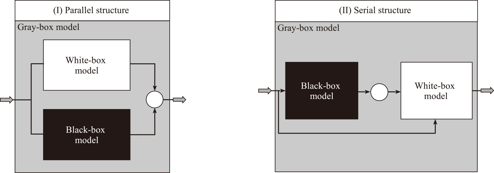
An improvement to the aforementioned drawback is the serial structure which uses the black-box model to be able to improve the uncertainties of the white-box model (Nazemzadeh et al., 2021). For example, it is conceivable to use the black-box model to predict the influence of flow conditions in a serial gray-box model structure or to correct separation-related properties, such as the hindered settling function, through on-line learning algorithms. However, this is challenging task and currently part of the research in the field of particle technology.
Fig. 11 shows experimental results of the solids mass fraction in the centrate of a pilot scale decanter centrifuge and simulation data based on a developed gray-box model based on a parallel structure. In this study, the white box model is the previously discussed 2D compartment model and the black box model corresponds to a neural network with one input, hidden and output layer. The training procedure of the neural network consists of a training and a test phase. The training data includes pilot test data for material properties measured at the feed, centrate and concentrate and the relevant process conditions.
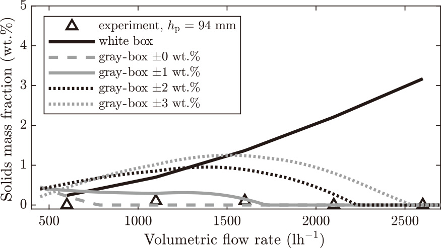
Another important point for the application of a gray-box model with parallel structure is the confidence interval necessary to allow the intervention of the black-box model when the white-box model has a poor accuracy. For the case presented in Fig. 11, there is a deviation of the white-box model at higher speeds. The smaller the confidence interval is set, the earlier the correction of the white-box model prediction by the black-box model occurs. As mentioned earlier, this allows the prediction of process behavior for decanter centrifuges to be improved by integrating experimental data.
6. Process analytics
Process monitoring is playing an increasingly important role in optimizing the operation of solid bowl centrifuges to achieve a higher product quality and shorter setup times. To avoid reject rates or exceeding tolerance limits, quality control is moving from off-line to on-line, or in-situ applications. On-line measurements typically use a bypass to guide the material into the measurement system. In contrast to off-line measurements, on-line detection requires both a sampling system and often a dilution station to measure particle properties with high accuracy. The following section summarizes several measurement methods for on-line and in-situ characterization of particle and bulk properties that have been applied to solid bowl centrifuges.
6.1 On-line measurement of particle properties
In tubular bowl centrifuges, the flow conditions change over time due to the accumulated solids. To maintain consistent product characteristics, the rotor speed or flow rate must be adjusted during the centrifugation process. However, in order to change the rotor speed, it is essential to monitor the particle properties at the centrate. For dilute suspensions, light scattering sensors are suitable to determine the solids volume fraction on-line (Konrath et al., 2014). To integrate such a system into the process, calibration with the initial suspension is required. Typically, a dilution series is necessary, which can be characterized by off-line measurements.
Fig. 12 illustrates the comparison of the product loss for the controlled (n controlled) and the non-controlled (n constant) scenario for a tubular bowl centrifuge type Z11. The controller design is based on the step response after changing solids volume fraction at the feed. A closer look at Fig. 12 reveals a fundamentally different process behavior for the non-controlled and the controlled case.
While the product loss increases with time for n = constant, since the machine fills continuously, the product loss remains constant for n = controlled. In this case, the decreasing residence time is compensated by increasing the rotational speed. Light scattering sensors can also be used to detect turbidity in the centrate of decanter and disk stack centrifuges to monitor centrate clarification and control the process to maintain product quality (Leung, 2007).
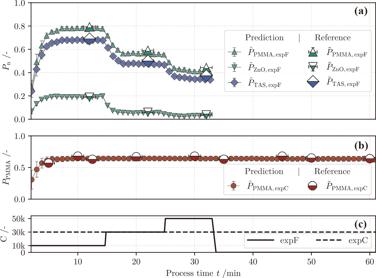
Another measurement system for on-line analysis of total suspended solids is UV-Vis spectroscopy. Unlike light scattering sensors, UV-Vis spectroscopy does not operate at a constant wavelength, but uses the full range of ultraviolet and visible light to produce an absorption spectrum. UV-Vis spectroscopy also requires extensive calibration based on a dilution series for the measured suspension. A promising technique to correlate the measured UV-Vis data with the solids volume fraction is the use of multivariate regression which is typically based on generalized ordinary least squares (Winkler et al., 2020). Another application of on-line UV-Vis spectroscopy is to detect the composition of binary mixtures (Winkler et al., 2021). One example is the on-line measurement of polymethyl methacrylate (PMMA) and zinc oxide (ZnO) in an aqueous system. Both particle systems consist of submicron particles. For composition prediction, both components must scatter a UV-Vis signal at different wavelengths. By directly coupling UV-Vis data with product-related properties such as the product loss, the UV-Vis sensor acts as a soft sensor that directly outputs the quality of a classification, or fractionation process (Winkler et al., 2021).
Fig. 13(a) shows the comparison between off-line and on-line measurement of the temporal change of the product loss for the fractionation of PMMA and ZnO. The results indicate a good agreement between reference values and the prediction also for the variation of the centrifugal number. Additionally, Fig. 13(b) illustrates the prediction of the temporal change of the product loss during the classification of a suspension consisting of PMMA and water.
Another method of recording the change in solids volume fraction in the centrate over time is to use a measuring cell with a light source and a camera system. The measured data can be evaluated using a convolutional neural network (CNN). Prediction requires a pre-trained CNN that has been trained with experimental data (Bai et al., 2021b). The presented deep learning algorithm is a hybrid neural network based on a CNN and a short-term memory network (LSTM). The LSTM helps to ensure that previous data is not forgotten, when searching for the correct gradients during the new training period (Bai et al., 2021b). The measuring system can be applied to a low concentrated suspension with a solids mass fraction of up to 0.5 wt %, which allows to detect the clarification in the centrate. On-line measurement of particle size distribution is challenging, but there are several methods such as laser diffraction, ultrasonic extinction, and X-ray. The practicality of an instrument depends on the particle properties, the solids volume fraction, and the process itself. If the measurement time is less than the residence time, the instrument can be used directly for process control after successful calibration. However, if the measurement time is longer than the residence time, the direct coupling of process control and measurement is challenging due to the different time scales. Furthermore, most particle size measurement techniques are only suitable for a defined particle size range, making experiments irreplaceable.
6.2 In-situ measurement of slurry properties
The in-situ measurement of particle properties in solid bowl centrifuges is very challenging due to the high centrifugal acceleration and requires costly sensors, but provides detailed information about the local physical behavior. Several aspects are necessary for the application of in-situ sensors in solid bowl centrifuges. First, gaps are needed inside the rotor to install the sensors. Therefore, it is necessary to calculate the influence of the gaps on the mechanical strength of the rotor. Second, signal transmission requires a transmitter, e.g., Wi-Fi, to transmit the measured signal to the receiver.
Wireless electrical resistance (WERD) is a technique to investigate sediment thickness at high relative centrifugal number (Prayitno et al., 2020). The measurement system records the change in electrical conductivity of the liquid phase in-situ by integrating multiple pairs of electrodes along the cylindrical conical bowl. The measured data can be used to indirectly calculate the solids volume fraction in the sediment.
An extension of this method is the Periodic Segmentation Technique in Wireless Electrical Resistance Detector (psWERD), which enables in-situ prediction of material functions such as the hindered settling function for decanter centrifuges. The periodic segmentation technique is necessary due to the influence of relative motion between the screw conveyor and the centrifuge bowl. The screw conveyor disturbs the measurement signal, due to the different material and is filtered by the periodic segmentation technique (Prayitno et al., 2022).
Another promising non-invasive and in-situ analysis of the sediment distribution is the Magnetic Resonance Imaging (MRI), which is an imaging technique based on the physical principle of nuclear magnetic resonance (Hardy, 2011). This is done by placing the rotor of the centrifuge in the tube of the tomograph.
In contrast to WERD or psWERD, the size of the tomography limits the application of MRI to small solid bowl centrifuges. An example of MRI is the study of sediment distribution in tubular bowl centrifuges (Spelter et al., 2013; Stahl et al., 2008). Fig. 14 (I) presents an adapted rotor of a tubular bowl centrifuge type GLE from CEPA. The rotor consists of a glass fiber reinforced plastic (GRP). The adapted rotor is necessary for the undisturbed MRI measurements of sediment distribution. The analysis of sediment involves a contrast agent such as carbon black (CB). CB generates a white contrast during MRI measurement, see Fig. 14 (II). A closer look at Fig. 14 (II) depicts that the temporal filling process starts from the right (inflow) to the left (centrate). The axial flow and the simultaneous classification of the particles along the rotor explain the non-uniform sediment build-up according to the previously mentioned CFD results and process simulation.

In summary, in-situ measurement methods provide very accurate insight into the physical behavior of solid bowl centrifuges, but experiments are time-consuming and equipment costs are high, limiting their use to research.
7. Conclusions
This work presented an overview of research in the field of modeling and optimization of solid bowl centrifuges. Modeling on different time and length scales helps to better understand the physical behavior of solid bowl centrifuges and optimize their operation. One of the major challenges in the selection and development of suitable models arises from the influence of distributed particle properties.
Conventional steady-state methods for the design of solid bowl centrifuges are based on several assumptions and are not predictive without several pilot scale experiments. The transfer from pilot to industrial scale is usually only possible for geometrically similar machines in combination with decades of experience of the manufacturers. A counter idea to conventional methods is to apply process modeling and to consider material functions for separation-related properties such as sedimentation, sediment build-up, and sediment transport. The measurement of the material properties is not carried out on the pilot but on a smaller laboratory scale, with well-established laboratory centrifuges. Furthermore, CFD helps to gain a better understanding of the usually inaccessible parts of a solid bowl centrifuge. At the same time, CFD can be used to optimize different centrifuge geometries, such as the feed accelerator or other parts of the machine.
However, since any form of modeling is based on assumptions and therefore does not completely reproduce the physics, there will always be deviations. This is where gray-box models have great potential to successively improve the modeling of solid bowl centrifuges. Data-driven methods such as supervised learning and neural networks allow an intensive analysis of process data.
Nevertheless, this requires the measurement of particle properties on-line or in-situ by integrating process analytics. Various measurement techniques such as turbidity or UV-Vis sensors, camera systems, laser diffraction, ultrasonic extinction and X-ray are available. However, due to the high cost of measuring equipment, individual testing of the particle system is necessary.
In summary, useful tools for the modeling and optimization of solid bowl centrifuges are available and their application has already been demonstrated in research. The task now is to further improve the algorithms and measurement methods. With further developments and the interconnection of gray-box models, process analytics, and advanced process control, the overriding goal of autonomous centrifugation will be possible in the future.
Acknowledgments
The authors gratefully acknowledge the funding by German Research Foundation (DFG) in the priority program SPP 1679 “Dynamic simulation of interconnected solids processes” and the Federal Ministry of Economic Affairs and Climate Action in the program IGF—Industrial Collective Research.
References
- Al-Naafá M.A., Selim M.S., Sedimentation of polydisperse concentrated suspensions, The Canadian Journal of Chemical Engineering, 67 (1989) 253–264. DOI:10.1002/cjce.5450670212
- Ambler C.M., The evaluation of centrifuge performance, Chemical Engineering Progress, 48 (1952) 150–158.
- Ambler C.M., The theory of scaling up laboratory data for the sedimentation type centrifuge, Journal of Microbial and Biochemical Technology, 1 (1959) 185–205. DOI:10.1002/jbmte.390010206
- Ambler C.M., The fundamentals of separation, including Sharples Sigma value for predicting equipment performance, Industrial and Engineering Chemistry Research, 48 (1961) 430–433.
- Anlauf H., Recent developments in centrifuge technology, Separation and Purification Technology, 58 (2007) 242–246. DOI:10.1016/j.seppur.2007.05.012
- Arcigni F., Friso R., Collu M., Venturini M., Harmonized and systematic assessment of microalgae energy potential for biodiesel production, Renewable and Sustainable Energy Reviews, 101 (2019) 614–624. DOI:10.1016/j.rser.2018.11.024
- Auzerais F.M., Jackson R., Russel W.B., The resolution of shocks and the effects of compressible sediments in transient settling, Journal of Fluid Mechanics, 195 (1988) 437–462. DOI:10.1017/S0022112088002472
- Bai C., Park H., Wang L., Modelling solid-liquid separation and particle size classification in decanter centrifuges, Separation and Purification Technology, 263 (2021a) 118408. DOI:10.1016/j.seppur.2021.118408
- Bai C., Park H., Wang L., Measurement of solids concentration in aqueous slurries for monitoring the solids recovery in solid bowl centrifugation, Minerals Engineering, 170 (2021b) 107068. DOI:10.1016/j.mineng.2021.107068
- Balbierer R., Gordon R., Schuhmann S., Willenbacher N., Nirschl H., Guthausen G., Sedimentation of lithium–iron–phosphate and carbon black particles in opaque suspensions used for lithium-ion-battery electrodes, Journal of Materials Science, 54 (2019) 5682–5694. DOI:10.1007/s10853-018-03253-2
- Beiser M., Bickert G., Scharfer P., Comparison of sedimentation behavior and structure analysis with regard to destabilization processes in suspensions, Chemical Engineering and Technology, 27 (2004) 1084–1088. DOI:10.1002/ceat.200403252
- Bell G.R.A., Pearse J.R., Experimental and computational analysis of the feed accelerator for a decanter centrifuge, Proceedings of the Institution of Mechanical Engineers, Part E: Journal of Process Mechanical Engineering, 230 (2016) 97–110. DOI:10.1177/0954408914539940
- Bell G.R.A., Symons D.D., Pearse J.R., Mathematical model for solids transport power in a decanter centrifuge, Chemical Engineering Science, 107 (2014) 114–122. DOI:10.1016/j.ces.2013.12.007
- Bhatty J.I., Clusters formation during sedimentation of dilute suspensions, Separation Science and Technology, 21 (1986) 953–967. DOI:10.1080/01496398608058389
- Bürger R., Concha F., Settling velocities of particulate systems: 12. Batch centrifugation of flocculated suspensions, International Journal of Mineral Processing, 63 (2001) 115–145. DOI:10.1016/S0301-7516(01)00038-2
- Buscall R., Mills P.D.A., Goodwin J.W., Lawson D.W., Scaling behaviour of the rheology of aggregate networks formed from colloidal particles, Journal of the Chemical Society, Faraday Transactions 1: Physical Chemistry in Condensed Phases, 84 (1988) 4249–4260. DOI:10.1039/F19888404249
- Byrne E.P., Fitzpatrick J.J., Pampel L.W., Titchener-Hooker N.J., Influence of shear on particle size and fractal dimension of whey protein precipitates: Implications for scale-up and centrifugal clarification efficiency, Chemical Engineering Science, 57 (2002) 3767–3779. DOI:10.1016/S0009-2509(02)00315-9
- Caponio F., Summo C., Paradiso V.M., Pasqualone A., Influence of decanter working parameters on the extra virgin olive oil quality, European Journal of Lipid Science and Technology, 116 (2014) 1626–1633. DOI:10.1002/ejlt.201400068
- Detloff T., Sobisch T., Lerche D., Particle size distribution by space or time dependent extinction profiles obtained by analytical centrifugation, Powder Technology, 174 (2007) 50–55. DOI:10.1016/j.powtec.2006.10.021
- Ekdawi N., Hunter R.J., Sedimentation of disperse and coagulated suspensions at high particle concentrations, Colloids and Surfaces, 15 (1985) 147–159. DOI:10.1016/0166-6622(85)80062-7
- Erk A., Anlauf H., Stahl W., Fließeigenschaften feinstdisperser, gesättigter Haufwerke während ihrer Kompression im Zentrifugalfeld, Chemie-Ingenieur-Technik, 76 (2004) 1494–1499. DOI:10.1002/cite.200407025
- Erk A., Luda B., Influencing sludge compression in solid-bowl centrifuges, Chemical Engineering and Technology, 27 (2004) 1089–1093. DOI:10.1002/ceat.200403260
- Esmaeilnejad-Ahranjani P., Hajimoradi M., Optimization of industrial-scale centrifugal separation of biological products: comparing the performance of tubular and disc stack centrifuges, Biochemical Engineering Journal, 178 (2022) 108281. DOI:10.1016/j.bej.2021.108281
- Ettmayr A., Bickert G., Stahl W., Zur Konzentrationsabhängigkeit des Sedimentationsvorgangs von Feinstpartikelsuspensionen in Zentrifugen, F+S Filtrieren u. Separieren, 15 (2001) 58–65.
- Faust T., Gösele W., Untersuchungen zur klärwirkung von dekantierzentrifugen, Chemie Ingenieur Technik, 57 (1985) 698–699. DOI:10.1002/cite.330570814
- Flegler A., Schneider M., Prieschl J., Stevens R., Vinnay T., Mandel K., Continuous flow synthesis and cleaning of nano layered double hydroxides and the potential of the route to adjust round or platelet nanoparticle morphology, RSC Advances, 6 (2016) 57236–57244. DOI:10.1039/c6ra09553d
- Flegler A., Wintzheimer S., Schneider M., Gellermann C., Mandel K., Tailored nanoparticles by wet chemical particle technology: from lab to pilot scale, in: Handbook of Nanomaterials for Industrial Applications, Elsevier, 2018, pp. 137–150.
- Frank U., Uttinger M.J., Wawra S.E., Lübbert C., Peukert W., Progress in multidimensional particle characterization, KONA Powder and Particle Journal, 39 (2022) 3–28. DOI:10.14356/kona.2022005
- Frost S., Neue Einblicke in die Abscheidung feiner Feststoffe in Dekantierzentrifugen, VDI-Verlag, 2000.
- Garrido P., Bürger R., Concha F., Settling velocities of particulate systems: 11. comparison of the phenomenological sedimentation-consolidation model with published experimental results, International Journal of Mineral Processing, 60 (2000) 213–227. DOI:10.1016/S0301-7516(00)00014-4
- Garrido P., Concha F., Bürger R., Settling velocities of particulate systems: 14. unified model of sedimentation, centrifugation and filtration of flocculated suspensions, International Journal of Mineral Processing, 72 (2003) 57–74. DOI:10.1016/S0301-7516(03)00087-5
- Ginisty P., Mailler R., Rocher V., Sludge conditioning, thickening and dewatering optimization in a screw centrifuge decanter: which means for which result?, Journal of Environmental Management, 280 (2021) 111745. DOI:10.1016/j.jenvman.2020.111745
- Gleiß M., Dynamische Simulation der Mechanischen Flüssigkeitsabtrennung in Vollmantelzentrifugen, KIT Scientific Publishing, Karlsruhe, 2018.
- Gleiss M., Hammerich S., Kespe M., Nirschl H., Application of the dynamic flow sheet simulation concept to the solid-liquid separation: separation of stabilized slurries in continuous centrifuges, Chemical Engineering Science, 163 (2017) 167–178. DOI:10.1016/j.ces.2017.01.046
- Gleiss M., Nirschl H., Dynamic simulation of mechanical fluid separation in solid bowl centrifuges, in: Dynamic Flowsheet Simulation of Solids Processes, 2020, pp. 237–268. DOI:10.1007/978-3-030-45168-4_7
- Göusele W., Schichtströmung in röhrenzentrifugen, Chemie Ingenieur Technik, 40 (1968) 657–659. DOI:10.1002/cite.330401307
- Green M.D., Eberl M., Landman K.A., Compressive yield stress of flocculated suspensions: determination via experiment, AIChE Journal, 42 (1996) 2308–2318. DOI:10.1002/aic.690420820
- Ha Z., Liu S., Settling velocities of polydisperse concentrated suspensions, Canadian Journal of Chemical Engineering, 80 (2002) 783–790. DOI:10.1002/cjce.5450800501
- Haller N., Greßlinger A.S., Kulozik U., Separation of aggregated β-lactoglobulin with optimised yield in a decanter centrifuge, International Dairy Journal, 114 (2021) 104918. DOI:10.1016/j.idairyj.2020.104918
- Haller N., Kulozik U., Separation of whey protein aggregates by means of continuous centrifugation, Food and Bioprocess Technology, 12 (2019) 1052–1067. DOI:10.1007/s11947-019-02275-1
- Hammerich S., Gleiß M., Kespe M., Nirschl H., An efficient numerical approach for transient simulation of multiphase flow behavior in centrifuges, Chemical Engineering & Technology, 41 (2018) 44–50. DOI:10.1002/ceat.201700104
- Hammerich S., Gleiß M., Nirschl H., Modeling and simulation of solid-bowl centrifuges as an aspect of the advancing digitization in solid-liquid separation, ChemBioEng Reviews, 6 (2019a) 108–118. DOI:10.1002/cben.201900011
- Hammerich S., Gleiss M., Stickland A.D., Nirschl H., A computationally-efficient method for modelling the transient consolidation behavior of saturated compressive particulate networks, Separation and Purification Technology, 220 (2019b) 222–230. DOI:10.1016/j.seppur.2019.03.060
- Hammerich S., Stickland A.D., Radel B., Gleiss M., Nirschl H., Modified shear cell for characterization of the rheological behavior of particulate networks under compression, Particuology, 51 (2020) 1–9. DOI:10.1016/j.partic.2019.10.005
- Hardy E.H., NMR Methods for the Investigation of Structure and Transport, Springer Science & Business Media, 2011.
- Hayakawa O., Nakahira K., Naito M., Tsubaki J.I., Experimental analysis of sample preparation conditions for particle size measurement, Powder Technology, 100 (1998) 61–68. DOI:10.1016/S0032-5910(98)00053-9
- Hirt C.W., Nichols B.D., Volume of fluid (VOF) method for the dynamics of free boundaries, Journal of Computational Physics, 39 (1981) 201–225. DOI:10.1016/0021-9991(81)90145-5
- Höfgen E., Teo H.E., Scales P.J., Stickland A.D., Vane-in-a-Filter and Vane-under-Compressional-Loading: novel methods for the characterisation of combined shear and compression, Rheologica Acta, 59 (2020) 349–363. DOI:10.1007/s00397-020-01193-w
- Horozov T.S., Binks B.P., Stability of suspensions, emulsions, and foams studied by a novel automated analyzer, Langmuir, 20 (2004) 9007–9013. DOI:10.1021/la0489155
- Janoske U., Piesche M., Numerische Simulation der Strömungsvorgänge und des Trennverhaltens von Suspensionen im freien Einzelspalt eines Tellerseparators, Chemie Ingenieur Technik, 71 (1999a) 249–253. DOI:10.1002/cite.330710315
- Janoske U., Piesche M., Numerical simulation of the fluid flow and the separation behavior in a single gap of a disk stack centrifuge, Chemical Engineering and Technology, 22 (1999b) 213–216. DOI:10.1002/(SICI)1521-4125(199903)22:3<213::AID-CEAT213>3.0.CO;2-C
- Jungbauer A., Continuous downstream processing of biopharmaceuticals, Trends in Biotechnology, 31 (2013) 479–492. DOI:10.1016/j.tibtech.2013.05.011
- Karolis A., Stahl W., An expanded mathematical model describing the conveying of pasty material in decanter centrifuges, in: 4th World Filtration Congress, 1986, pp. 9.9–9.16.
- Kempken R., Preissmann A., Berthold W., Assessment of a disc stack centrifuge for use in mammalian cell separation, Biotechnology and Bioengineering, 46 (1995) 132–138. DOI:10.1002/bit.260460206
- Khatib Z.I., Faucher M.S., Sellman E.L., Field evaluation of disc-stack centrifuges for separating oil/water emulsions on offshore platforms, in: SPE Annual Technical Conference and Exhibition, 1995.
- Kohsakowski S., Seiser F., Wiederrecht J.-P.pdfilip., Reichenberger S., Vinnay T., Barcikowski S., Marzun G., Effective size separation of laser-generated, surfactant-free nanoparticles by continuous centrifugation, Nanotechnology, 31 (2019) 95603. DOI:10.1088/1361-6528/ab55bd
- König J., Janssen N., Janoske U., Visualization of the deposition mechanisms in disk stack centrifuges with an acrylic glass bowl top and high-speed image processing, Separation Science and Technology, 56 (2021) 640–652. DOI:10.1080/01496395.2020.1728326
- König J., Ueding J., Janoske U., Analytical model to characterize the efficiency of disk stack separators, Chemie-Ingenieur-Technik, 92 (2020) 701–710. DOI:10.1002/cite.201900177
- Konrath M., Brenner A.-K., Dillner E., Nirschl H., Centrifugal classification of ultrafine particles: Influence of suspension properties and operating parameters on classification sharpness, Separation and Purification Technology, 156 (2015) 61–70. DOI:10.1016/j.seppur.2015.06.015
- Konrath M., Gorenflo J., Hübner N., Nirschl H., Application of magnetic bearing technology in high-speed centrifugation, Chemical Engineering Science, 147 (2016) 65–73. DOI:10.1016/j.ces.2016.03.025
- Konrath M., Hackbarth M., Nirschl H., Process monitoring and control for constant separation conditions in centrifugal classification of fine particles, Advanced Powder Technology, 25 (2014) 991–998. DOI:10.1016/j.apt.2014.01.022
- Kynch G.J., A theory of sedimentation, Transactions of the Faraday Society, 48 (1952) 166–176. DOI:10.1039/tf9524800166
- Landman K.A., White L.R., Eberl M., Pressure filtration of flocculated suspensions, AIChE Journal, 41 (1995) 1687–1700. DOI:10.1002/aic.690410709
- Lester D.R., Usher S.P., Scales P.J., Estimation of the Hindered Settling Function from Batch-Settling Tests, 51 (2005) 1158–1168. DOI:10.1002/aic.10333
- Leung W.F., New decanter centrifuge technology for improved separation and high throughput, Fluid-Particle Separations Journal, 16 (2004) 37–51.
- Leung W.W.-F., Industrial Centrifugation Technology, McGraw-Hill, New York, 1998, ISBN: 9780070371910.
- Leung W.W.F., Separation of dispersed suspension in rotating test tube, Separation and Purification Technology, 38 (2004) 99–119. DOI:10.1016/j.seppur.2003.10.003
- Leung W.W.F., Centrifugal Separations in Biotechnology, Elsevier Science, 2007, ISBN: 978-1-85617-477-0. DOI:10.1016/B978-1-85617-477-0.X5000-9
- Lopes A.G., Keshavarz-Moore E., Ultra scale-down device to predict dewatering levels of solids recovered in a continuous scroll decanter centrifuge, Biotechnology Progress, 29 (2013) 1494–1502. DOI:10.1002/btpr.1814
- Menesklou P., Nirschl H., Gleiss M., Dewatering of finely dispersed calcium carbonate-water slurries in decanter centrifuges: about modelling of a dynamic simulation tool, Separation and Purification Technology, 251 (2020) 117287. DOI:10.1016/j.seppur.2020.117287
- Menesklou P., Sinn T., Nirschl H., Gleiss M., Grey box modelling of decanter centrifuges by coupling a numerical process model with a neural network, Minerals, 11 (2021a) 755. DOI:10.3390/min11070755
- Menesklou P., Sinn T., Nirschl H., Gleiss M., Scale-up of decanter centrifuges for the particle separation and mechanical dewatering in the minerals processing industry by means of a numerical process model, Minerals, 11 (2021b) 1–18. DOI:10.3390/min11020229
- Merkl R., Steiger W., Properties of decanter centrifuges in the mining industry, Minerals and Metallurgical Processing, 29 (2012) 6–12. DOI:10.1007/bf03402327
- Michaels A., Bolger J., Settling rates and sediment volumes of flocculated kaolin suspensions, Industrial & Engineering Chemistry Fundamentals, 1 (1962) 24–33. DOI:10.1021/i160001a004
- Mladenchev T., Modellierung des Filtrations- und Fließverhaltens von ultrafeinen, kompressiblen, flüssigkeitsgesättigten Partikelpackungen, Otto-von-Guericke-Universität Magdeburg, 2007.
- Najjar Y.S.H., Abu-Shamleh A., Harvesting of microalgae by centrifugation for biodiesel production: a review, Algal Research, 51 (2020) 102046. DOI:10.1016/j.algal.2020.102046
- Nazemzadeh N., Malanca A.A., Nielsen R.F., Gernaey K.V., Andersson M.P., Mansouri S.S., Integration of first-principle models and machine learning in a modeling framework: an application to flocculation, Chemical Engineering Science, 245 (2021) 116864. DOI:10.1016/j.ces.2021.116864
- Neumann A., Hoyer W., Wolff M.W., Reichl U., Pfitzner A., Roth B., New method for density determination of nanoparticles using a CPS disc centrifugeTM, Colloids and Surfaces B: Biointerfaces, 104 (2013) 27–31. DOI:10.1016/j.colsurfb.2012.11.014
- Peth S., Applications of microtomography in soils and sediments, in: Developments in Soil Science, Elsevier, 2010, pp. 73–101. DOI:10.1016/S0166-2481(10)34003-7
- Prayitno Y.A.K., Sejati P.A., Zhao T., Iso Y., Kawashima D., Takei M., In situ measurement of hindered settling function in decanter centrifuge by periodic segmentation technique in wireless electrical resistance detector (psWERD), Advanced Powder Technology, 33 (2022) 103370. DOI:10.1016/j.apt.2021.11.022
- Prayitno Y.A.K., Zhao T., Iso Y., Takei M., In situ measurement of sludge thickness in high-centrifugal force by optimized particle resistance normalization for wireless electrical resistance detector (WERD), Measurement Science and Technology, 32 (2020) 034001. DOI:10.1088/1361-6501/abc108
- Quemada D., Rheology of concentrated disperse systems and minimum energy dissipation principle, Rheologica Acta, 16 (1977) 82–94. DOI:10.1007/BF01516932
- Radel B., Gleiß M., Nirschl H., Crystal breakage due to combined normal and shear loading, Crystals, 12 (2022) Article no: 644. DOI:10.3390/cryst12050644
- Rathore A.S., Agarwal H., Sharma A.K., Pathak M., Muthukumar S., Continuous processing for production of biopharmaceuticals, Preparative Biochemistry and Biotechnology, 45 (2015) 836–849. DOI:10.1080/10826068.2014.985834
- Records A., Sutherland K., Decanter Centrifuge Handbook, Elsevier Science, 2001, ISBN:9781856173698.
- Reif F.R., Stahl W., Transportation of moist solids in decanter centrifuges, Chemical Engineering Progress, 85 (1989) 57–67.
- Reuter H., Sedimentation in der Überlaufzentrifuge, Chemie Ingenieur Technik, 39 (1967) 548–553. DOI:10.1002/cite.330390910
- Richardson J.F., Zaki W.N., The sedimentation of a suspension of uniform spheres under conditions of viscous flow, Chemical Engineering Science, 3 (1954) 65–73. DOI:10.1016/0009-2509(54)85015-9
- Richardson J.F., Zaki W.N., Sedimentation and fluidisation: part I, Chemical Engineering Research and Design, 75 (1997) S82–S100. DOI:10.1016/S0263-8762(97)80006-8
- Romani Fernández X., Prediction of multiphase flow and separation efficiency of industrial centrifuges by means of numerical simulation, Karlsruher Institut für Technologie (KIT), 2012, ISBN: 9783954041527.
- Romaní Fernández X., Nirschl H., A numerical study of the impact of radial baffles in solid bowl centrifuges using computational fluid dynamics, Physical Separation in Science and Engineering, (2010) 510570. DOI:10.1155/2010/510570
- Romaní Fernández X., Nirschl H., Multiphase CFD simulation of a solid bowl centrifuge, Chemical Engineering & Technology, 32 (2009) 719–725. DOI:10.1002/ceat.200800531
- Romaní Fernández X., Nirschl H., Fernández X.R., Nirschl H., Simulation of particles and sediment behaviour in centrifugal field by coupling CFD and DEM, Chemical Engineering Science, 94 (2013) 7–19. DOI:10.1016/j.ces.2013.02.039
- Schubert T., Meric A., Boom R., Hinrichs J., Atamer Z., Application of a decanter centrifuge for casein fractionation on pilot scale: effect of operational parameters on total solid, purity and yield in solid discharge, International Dairy Journal, 84 (2018) 6–14. DOI:10.1016/j.idairyj.2018.04.002
- Shekhawat L.K., Sarkar J., Gupta R., Hadope S., Application of CFD in bioprocessing: separation of mammalian cells using disc stack centrifuge during production of biotherapeutics, Journal of Biotechnology, 267 (2018) 1–11. DOI:10.1016/j.jbiotec.2017.12.016
- Sinn T., Flegler A., Wolf A., Stübinger T., Witt W., Nirschl H., Gleiß M., Investigation of centrifugal fractionation with time-dependent process parameters as a new approach contributing to the direct recycling of lithium-ion battery components, Metals, 10 (2020) 1–18. DOI:10.3390/met10121617
- Skinner S.J., Stickland A.D., White L.R., Lester D.R., Shane P., Analysis of centrifugal settling of strongly flocculated suspensions, in: 12th World Filtration Congress, 2016.
- Sobisch T., Kavianpour D., Lerche D., Characterization of solid-liquid separation of flocculated mineral slurries by NIR-transmission and X-ray concentration profiling, Proceedings Filtech Köln, Germany, 2016. https://papers.ssrn.com/sol3/papers.cfm?abstract_id=2977872
- Spelter L.E., Nirschl H., Stickland A.D., Scales P.J., Pseudo two-dimensional modeling of sediment build-up in centrifuges: a compartment approach using compressional rheology, AIChE Journal, 59 (2013) 3843–3855. DOI:10.1002/aic.14115
- Spelter L.E., Schirner J., Nirschl H., A novel approach for determining the flow patterns in centrifuges by means of laser-doppler-anemometry, Chemical Engineering Science, 66 (2011) 4020–4028. DOI:10.1016/j.ces.2011.05.022
- Spelter L.E., Steiwand A., Nirschl H., Processing of dispersions containing fine particles or biological products in tubular bowl centrifuges, Chemical Engineering Science, 65 (2010) 4173–4181. DOI:10.1016/j.ces.2010.04.028
- Stahl S., Spelter L.E., Nirschl H., Investigations on the separation efficiency of tubular bowl centrifuges, Chemical Engineering & Technology, 31 (2008) 1577–1583. DOI:10.1002/ceat.200800300
- Stahl W., Langeloh T., Improvement of clarification in decanting centrifuges, German Chemical Engineering, 55 (1983) 324–325. DOI:10.1002/cite.330550423
- Stahl W.H., Fest-Flüssig-Trennung Band II: Industrie-Zentrifugen, Maschinen- Und Verfahenstechnik, DRM Press, CH-Männedorf, 2004, ISBN:9783952279403.
- Stokes G.G., On the effect of the internal friction of fluids on the motion of pendulums, Transactions of the Cambridge Philosophical Society, 9 (1850).
- Törnblom O., Turbulent shear and breakup of flocculated biomaterial in centrifuge inlets, Chemical Engineering & Technology, 41 (2018) 2366–2374. DOI:10.1002/ceat.201800297
- Usher S.P., Studer L.J., Wall R.C., Scales P.J., Characterisation of dewaterability from equilibrium and transient centrifugation tests data, Chemical Engineering Science, 93 (2013) 277–291. DOI:10.1016/j.ces.2013.02.026
- Wakeman R.J., Separation technologies for sludge dewatering, Journal of Hazardous Materials, 144 (2007) 614–619. DOI:10.1016/j.jhazmat.2007.01.084
- Winkler M., Gleiss M., Nirschl H., Soft sensor development for real-time process monitoring of multidimensional fractionation in tubular centrifuges, Nanomaterials, 11 (2021). DOI:10.3390/nano11051114
- Winkler M., Sonner H., Gleiss M., Nirschl H., Fractionation of ultrafine particles: Evaluation of separation efficiency by UV–vis spectroscopy, Chemical Engineering Science, 213 (2020) 115374. DOI:10.1016/j.ces.2019.115374
- Wolf A., Flegler A., Prieschl J., Stuebinger T., Witt W., Seiser F., Vinnay T., Sinn T., Gleiß M., Nirschl H., et al., Centrifugation based separation of lithium iron phosphate (LFP) and carbon black for lithium-ion battery recycling, Chemical Engineering and Processing-Process Intensification, 160 (2021) 108310. DOI:10.1016/j.cep.2021.108310
- Xiong Q., Jutan A., Grey-box modelling and control of chemical processes, Chemical Engineering Science, 57 (2002) 1027–1039. DOI:10.1016/s0009-2509(01)00439-0
- Yoshida H., Masuda H., Fukui K., Tokunaga Y., Particle size measurement with an improved sedimentation balance method and microscopic method together with computer simulation of necessary sample size, Advanced Powder Technology, 12 (2001) 79–94. DOI:10.1163/156855201744976
- Zhu G., Tan W., Yu Y., Liu L., Experimental and numerical study of the solid concentration distribution in a horizontal screw decanter centrifuge, Industrial & Engineering Chemistry Research, 52 (2013) 17249–17256. DOI:10.1021/ie401902m
- Zhu M., Hu D., Xu Y., Zhao S., Design and computational fluid dynamics analysis of a three-phase decanter centrifuge for oil-water-solid separation, Chemical Engineering and Technology, 43 (2020) 1005–1015. DOI:10.1002/ceat.201900245
Authors’ Short Biographies
Marco Gleiss

Marco Gleiss has studied Chemical Engineering at the Karlsruhe Institute of Technology (KIT) and subsequently became a doctoral student at the Institute of Mechanical Process Engineering and Mechanics (KIT), where he got his Ph.D in Chemical Engineering and became Senior scientist. His research interest is in the field of solid–liquid separation, on the digitization of filtration and centrifugation, the development of digital twins, and autonomous processes.
Hermann Nirschl

Hermann Nirschl received his Ph.D. in fluid mechanics from the Technical University in Munich in 1994. In the years between 1997 and 2003 he was responsible for process engineering developments for the 3M company. From 2003 on he is Professor for Mechanical Process Engineering at the KIT. The focus of the research is on particle technology with a special emphasis on separation processes, numerical simulation and the development of particle characterization technologies.
 https://ror.org/04t3en479

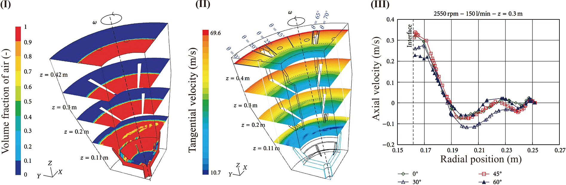

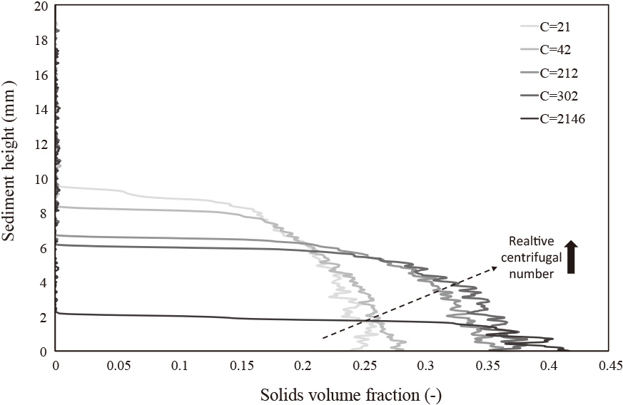
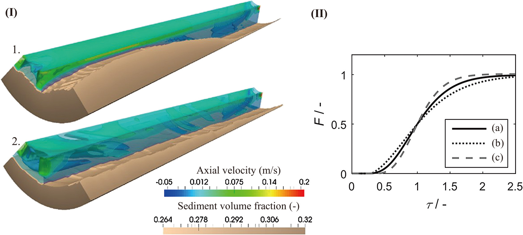
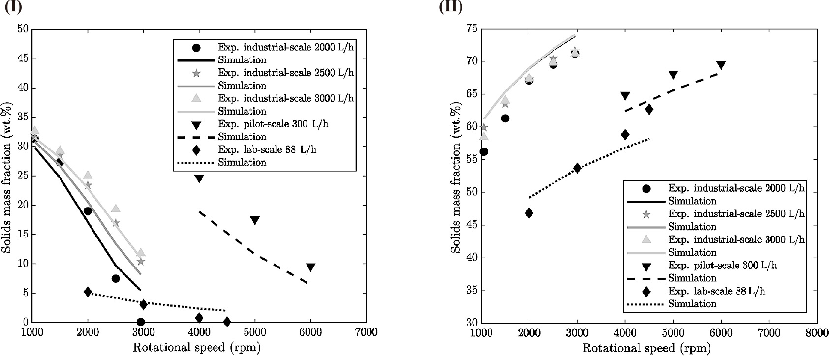

;%0A%09%09%09newWindow.document.open();%0A%09%09%09newWindow.document.write('<img src=%22./Graphics/41_2024010_15.jpg%22>');%0A%09%09%09newWindow.document.close();%0A%09%09)
;%0A%09%09%09newWindow.document.open();%0A%09%09%09newWindow.document.write('<img src=%22./Graphics/41_2024010_16.jpg%22>');%0A%09%09%09newWindow.document.close();%0A%09%09)