Materials Processing
Numerical Analysis of Fillet Shape and Molten Filler Flow during Brazing in the Al–Si Alloy of Automotive Radiator
2021 Volume 62 Issue 4 Pages 498-504

Details
2021 Volume 62 Issue 4 Pages 498-504
In the brazing process of an automobile radiator, eutectic melting of the Al–Si filler alloy of the clad sheets, fillet formation in the brazed joints, and the flow of the molten filler metal on the solid core metal between joints occur continuously. With regard to designing heat exchangers, the optimum placement of the filler metal, considering the flow of the molten filler metal, is an important subject. In this study, a new numerical analysis was applied to predict the shape of the fillets and the molten filler flow. The molten filler flow was calculated using the difference method applied to a one-dimensional unsteady flow that is assumed to be a uniform flow of incompressible viscous fluid between two parallel plates. Among some numerical results, when the hydraulic mean depth of the flow path was reduced 0.3 times, the calculation results were consistent with the actual values. It was necessary to narrow the flow path because it was calculated assuming that the flow of brazing was between two parallel flat plates, whereas the actual flow path of the molten filler metal was not flat and a large flow resistance was produced.
Comparison of actual and numerical data for fillet membrane at each joint.
Aluminum heat exchangers for automotive applications are widely manufactured using a vacuum or controlled atmosphere brazing.1) The brazing sheets comprising an Al–Mn series core alloy cladded with an Al–Si series filler alloy are used in tubes and fins components. In recent years, since the thickness of the brazing sheets has been decreasing with the weight reduction of the heat exchangers,2,3) the quantity of filler metal supplied to the joint has been decreasing. In addition, even if a sufficient quantity of filler metal would be placed near each joint prior to brazing, the individual size of the fillet at a joint would be insufficient because the molten filler metal does not stay in the intended joint but flows to other joints. Therefore, in the design and manufacture of heat exchangers, the optimum placement of the filler metal, considering the molten filler flow, is an important subject to form sufficient fillets in the brazed joints. However, the filler flow during brazing between joints is not fully understood. To overcome this problem, it is effective to predict the quantity of the molten filler and the fillet shape at each joint during brazing. Furthermore, the prediction of the filler flow is very useful to optimize the brazing conditions and reduce brazing defects.
Concerning the prediction of the fillet shape, there have been some numerical analyses based on the finite element method, in which the summation of surface energy, potential energy, and interface energy of the fillet was minimized.4–6) According to these results, the actual values and the calculated values of the fillet shape were in good agreement. For the prediction of the molten filler flow, a study examined the phenomenon in which molten AA4343 filler flowed through the artificial micro groove formed on the AA3003 substrate.7) The results showed that the actual flow distance of the molten filler was smaller than that of the calculated value based on the modified version of the capillary flow model of Washburn,8) advanced by Yost et al.9) In this study, since the single groove model simplified the molten filler flow, it was impossible to predict the complicated molten filler flow of the actual heat exchangers.
Computational fluid dynamics has been used and applied in various technical fields, and there has been an example of numerical analysis of water flow in underground diversion channels.10) The primary feature of this particular study is the unsteady flow of water in the main tunnel and the simultaneously changing water level in the vertical shafts connected to the main tunnel. The molten filler flow is considered to be similar to the flow in underground diversion channels. This is because the molten filler flow on the surface of the tube material is equivalent to the water flow in the main tunnel, and the transformation of the fillet shape is equivalent to the changing water level in the vertical shaft. Although it is difficult to calculate the molten filler flow using the same analytical model of the underground diversion channel, it is possible to apply the discretization method of this model to the molten filler flow model.
This paper describes a unique numerical model of the fillet shape and the molten filler flow during brazing for an automotive radiator with reference to the water flow in underground diversion channels. Subsequently, the fillet shape of the actual radiator was compared with the calculated value. Based on the results, the growth of the fillet with increasing temperature during brazing is discussed.
The fillet shape was measured using a radiator that was brazed in an inert gas atmosphere while measuring the temperature of the plate and the tube. The radiator consists of a press-formed header plate, a welded oval tube, and a corrugated fin, as shown in Fig. 1. The header plate was made of a brazing sheet with a thickness of 1.2 mm, composed of a 3000 series alloy core material cladded with AA4343 (Al–7.5 mass%Si) of 10% clad ratio. The tube was also made of the brazing sheet above mentioned with a thickness of 0.23 mm, and with AA4045 (Al–10.0 mass%Si) of 13% clad ratio. The fin was made of a 3000 series bare sheet with a thickness of 0.05 mm. The brazing condition was an oxygen concentration of 100 ppm or less and the maximum temperatures of 867 K and 869 K for the plate and the tube in the center of the core, respectively.
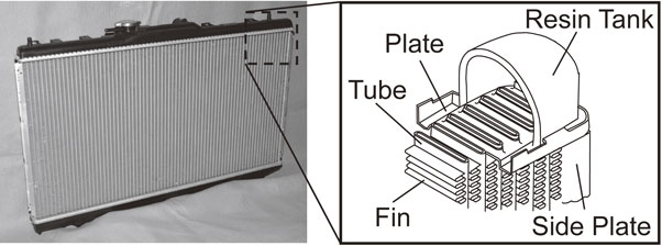
Components of an automotive radiator.
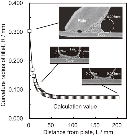
The tube at the center of the core was cut out along with the plate and fins, and the cross-section microstructure of the plate-tube joint and the fin-tube joint were observed at the center of the tube width. The curvature radius of the fillet was measured by image analysis of the cross-section microstructure. The curvature radii of the twenty fin-tube fillets located within 50 mm from the plate-tube joint were measured continuously. In addition, the curvature radii of the fillet at the fin-tube every 25 mm, located 50–200 mm from the plate-tube joint, were also measured. Figure 2(a) shows the fillet at the plate-tube joint, and Fig. 2(b) and (c) show the fillets at the fin-tube joints, located at 15.5 mm and 200.0 mm from the plate-tube joint. The numbers in the figure show the measured curvature radius of each fillet. The near and far sides of the fin-tube joint in Fig. 2(b) demonstrate the positional relationship from the plate-tube joint.

Cross sections and curvature radii of fillets at joints. (a) Plate-tube joint. Fin-tube joints located at (b) 15.5 mm and (c) 200.0 mm from the plate-tube joint.
Numerical analysis of the fillet shape and the molten filler flow was performed according to the flow chart in Fig. 3. These calculations were based on the following assumptions:
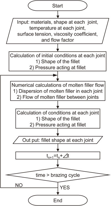
Flow chart for numerical analysis of the fillet shape and the filler flow.
The specifications of the plate, tube, and fin materials are the same as those of the actual radiator, as shown above. The shapes of the plate-tube and fin-tube joints are traced from the cross-sections shown in Fig. 2 by image analysis. With regard to the shapes of fin-tube joints, since the fin shapes were different depend on each joint, these shapes were adjusted to the one average shape. The brazing temperature at the plate-tube joint TP and the fin-tube joint TF was obtained from the actual measurement results shown in Fig. 4. To simplify the calculations, the time elapsed during the cooling phase has been removed from the brazing temperature cycle.
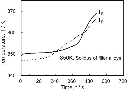
Temperature-time curve during brazing, excluding the cooling phase.
It is assumed that the fillets are formed by absorbing the molten filler through capillary action along the gap between the two members forming the joint. Figure 5 shows the schematic of the fillet between part 1 and part 2. The schematic of the fillet surface, defined by a circular arc whose center is located at coordinates (X0, Y0), can be described as
| \begin{equation} X = R\cos \theta + X_{0} \end{equation} | (1) |
| \begin{equation} Y = R\sin \theta + Y_{0} \end{equation} | (2) |
| \begin{equation} X_{\textit{part}1} = R\cos \theta_{1} + X_{0} \end{equation} | (3) |
| \begin{equation} f_{\textit{part}1}(X_{\textit{part}1}) = R\sin \theta_{1} + Y_{0} \end{equation} | (4) |
| \begin{equation} {-}1/\tan \theta_{1} = df_{\textit{part}1}(X_{\textit{part}1})/dx + \tan \theta_{\textit{part}1} \end{equation} | (5) |
| \begin{equation} {-}1/\tan \theta_{2} = df_{\textit{part}2}(X_{\textit{part}2})/dx - \tan \theta_{\textit{part}2} \end{equation} | (6) |
| \begin{align} S &= 1/2\left|\sum\nolimits_{j=1}^{n}(X_{j} - X_{j+1})(Y_{j} + Y_{j+1})\right| \\ &\quad - R^{2}/2\int\nolimits_{\theta_{1}}^{\theta_{2}}\cos^{2}\theta d\theta \end{align} | (7) |
| \begin{equation} V = S \cdot w_{\textit{joint}} \end{equation} | (8) |
Schematic of fillet used for calculations.
Initial condition of the membrane of fillet between fin-tube joints.
Figure 7 shows a schematic model of a tube in the radiator with a fin and plate, for numerical calculation. This is a half-tube model based on the longitudinal symmetry of a real radiator tube. There are one plate-tube joint and sixty-seven fin-tube joints. As shown in Fig. 8, the region was divided so that each element included only one joint. The element at i = 0 is the plate-tube joint and the elements at i = 1 to 67 are the fin-tube joints. A continuity equation calculates the fillet volume at each element under the conditions that give the inflow and outflow of the molten filler at the joint. Thus, the continuity equation can be described as
| \begin{equation} dV_{i}/dt = \textit{Qmelt}_{i} + Q_{i} - Q_{i + 1} \end{equation} | (9) |
| \begin{equation} \partial Q/\partial x = \partial (uA)/\partial x = 0 \end{equation} | (10) |
| \begin{equation} \rho(\partial u/\partial t + u\partial u/\partial x) = -\partial P/\partial x + \mu \partial^{2}u/\partial x^{2} \end{equation} | (11) |
| \begin{equation} P = \gamma/R \end{equation} | (12) |
Symmetric model of the tube with fin and plate.

Mesh division of joints for calculation.
Assuming that the flow of the molten filler is a steady flow of incompressible viscous fluid between two parallel flat plates and the motion of the molten filler in the fillet is neglected, the average flow rate Qave obtained from eqs. (10) and (11) is described as
| \begin{equation} Q_{\textit{ave}} = w(\alpha d)^{3}\Delta P/12\mu L \end{equation} | (13) |
| \begin{equation} \textit{Qmelt}_{i} = - w(\alpha d_{i})^{3}P_{i}/12\mu L_{i} - w(\alpha d_{i+1})^{3}P_{i}/12\mu L_{i+1} \end{equation} | (14) |
| \begin{equation} Q_{i} = w(\alpha d_{i})^{3}(P_{i-1} - P_{i})/12\mu L_{i} \end{equation} | (15) |
| \begin{equation} V_{i}^{n+1} = V_{i}^{n} + (\textit{Qmelt}_{i}^{n} + Q_{i}^{n} - Q_{i+1}^{n})\Delta t \end{equation} | (16) |
| \begin{align} V_{i}^{n+1} &= V_{i}^{n} + [\{-w(\alpha d_{i}^{n})^{3}P_{i}^{n}/12\mu_{i}^{n}L_{i} \\ &\quad - w(\alpha d_{i+1}^{n})^{3}P_{i}^{n}/12\mu_{i}^{n}L_{i+1}\} \\ &\quad + w(\alpha d_{i}^{n})^{3}(P_{i-1}^{n} - P_{i}^{n})/12\mu_{i}^{n}L_{i}\\ &\quad - w(\alpha d_{i+1}^{n})^{3}(P_{i}^{n} - P_{i+1}^{n})/12\mu_{i}^{n}L_{i+1}]\Delta t \end{align} | (17) |
| \begin{align} d_{i}^{n+1} &= d_{i}^{n} - \{-w(\alpha d_{i}^{n})^{3}P_{i-1}^{n}/12\mu_{i}^{n}L_{i} \\ &\quad - w(\alpha d_{i}^{n})^{3}P_{i}^{n}/12\mu_{i}^{n}L_{i}\}\Delta t/wL_{i} \end{align} | (18) |
| \begin{equation} \mu_{i=0}^{n} = -0.0060T_{P}^{n} + 3.6795 \quad T \geq 850\,\text{K} \end{equation} | (19) |
| \begin{equation} \mu_{i \geq 1}^{n} = -0.0175T_{F}^{n} + 10.3104 \quad T \geq 850\,\text{K} \end{equation} | (20) |
The quantity of molten filler at every temperature during the brazing process was calculated by multiplying the flow factor $K_{i}^{n}$ by the filler volume prior to brazing. The flow factor is calculated according to the Si concentration of the brazing material using the Lagrange complement polynomial, based on the actual data at various Si concentrations shown in Fig. 9.13) In the AA4343 plate filler case, the value of the dotted line is entered into $K_{i = 0}^{n}$. In the case of the AA4045 tube filler, the corrected value of the dashed line is entered into $K_{i \geq 1}^{n}$. The actual data were measured when the clad thickness of filler was 0.12 mm, although the clad thickness of the tube filler was 0.03 mm, so the flow factor of AA4045 was reduced from the dotted line of AA4045 to the dashed line of the corrected AA4045. This is because the molten filler amount decreases with the decrease of the filler thickness owing to the diffusion of Si elements in the filler alloy to the core alloy during brazing. The total absorbed molten filler does not exceed the quantity of the molten filler obtained from the flow factor because the molten filler generated between the (i − 1)th and ith joints is absorbed into both the (i − 1)th and ith joints. This relation is described as
| \begin{align} K_{i}^{n}wt_{\textit{clad},i}L_{i} &\geq \sum\nolimits_{n}\{-w(\alpha d_{i}^{n})^{3}P_{i-1}^{n}/12\mu_{i}^{n}L_{i} \\ &\quad - w(\alpha d_{i}^{n})^{3}P_{i}^{n}/12\mu_{i}^{n}L_{i}\}\Delta t \end{align} | (21) |
Experimental and calculated flow factor of Al–Si series filler alloy.
The volume of the fillet at each element is calculated by the one-dimensional forward difference method by combining eqs. (17)–(21) at every 0.02 sec time step, and then the fillet shapes are determined using the volumes of the fillets, as described in section 2.2.2. $V_{i}^{0}$ and $P_{i}^{0}$ as the initial conditions are assigned the minimum value obtained from the calculated minimum fillet shape of each joint, as shown in Fig. 6. $d_{i}^{0}$ is the clad thickness of the plate and tube prior to brazing. The boundary conditions are $Q_{0}^{n} = 0$ and $Q_{67}^{n} = 0$, indicating a zero flow rate at both ends of the tube. The numerical analysis was executed using a self-build code on Visual Basic for Applications software.
Figure 10 shows the curvature radii of the fillet at the plate-tube and fin-tube joints. In Fig. 10, there are two dots in the plate-tube joint on the front and rear side where the measurement was made. In the fin-tube joints, the values were also measured at both the front and rear side, and these values are in average the curvature radii of the near and the far side as shown in Fig. 2(b). The maximum value of the curvature radius among all joints was 0.322 mm measured at the plate-tube joint. The curvature radii at the fin-tube joints within 75 mm from the plate-tube joint decreased non-linearly from 0.180 mm to 0.070 mm with the distance from the plate-tube joint. The curvature radii at the fin-tube joints located at more than 75 mm from the plate-tube joint became steady value around 0.070 mm. According to these results, it is considered that the molten filler of the plate flowed through the tube surface within 75 mm from the plate-tube joint, and the fillets of fin-tube joints were formed from the filler of both plate and tube. On the other hand, for the fin-tube joints located at more than 75 mm from the plate-tube joint, it is considered that the fillets were formed from only the filler of the nearest tube surface.
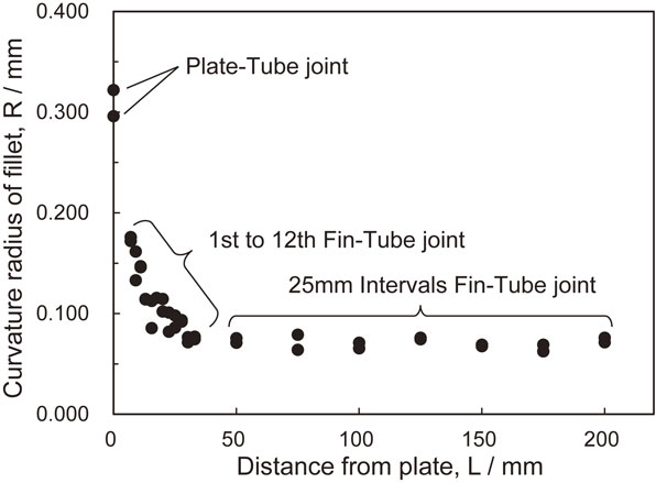
Distribution of curvature radius of the actual fillet at the plate-tube and fin-tube joints.
The actual value and numerical model of the fillet shape of the plate-tube and fin-tube joints are shown in Fig. 11(a) and (b), respectively. The actual values were measured from Fig. 2(a) and (c). The numerical models were determined by adjusting the fillet areas, considering the actual value; the contact angles were 0°, 20°, and 40°, respectively. In the plate-tube joint, the fillet shape of each contact angle corresponded to the actual value. The fillet shape corresponding to the contact angle of 0° was the best match among all the contact angles for the actual value. The result for the fin-tube joint was the same as that of the plate-tube joint. According to these results, it is appropriate to represent the molten filler surface through a simple circular arc. In the case of a curvature radius of less than 0.300 mm, the bond number Bo, indicating the ratio of gravity to surface tension, is less than 0.01, and the effect of gravity becomes extremely small. The reason for the best match of the measurement value at a contact angle of 0° with the numerical model was attributed to the surface tension of solid aluminum being sufficiently larger than that of liquid aluminum under good brazing conditions.
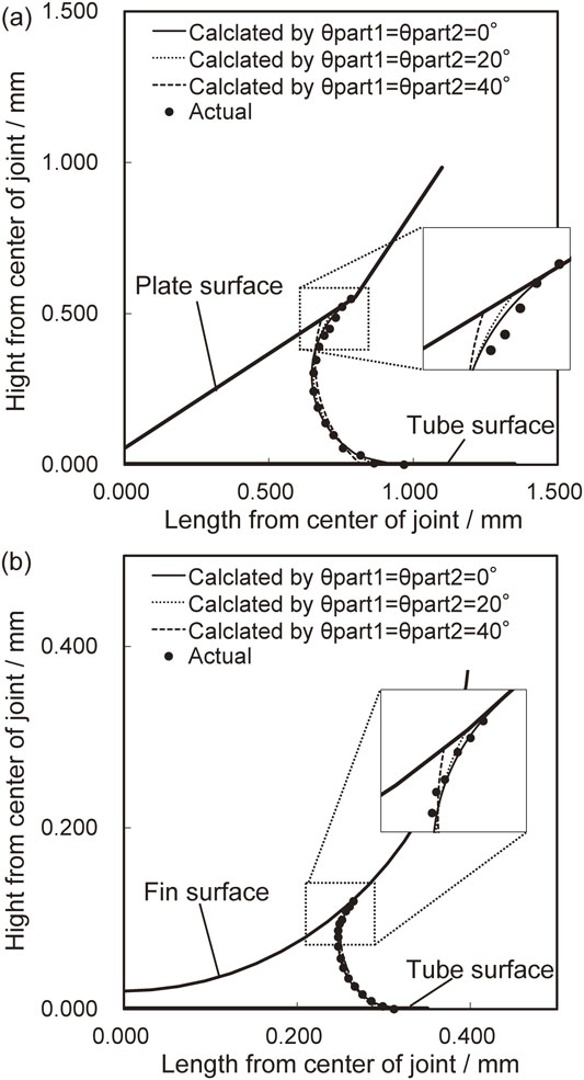
Comparison of actual and calculated data for the fillet membrane at (a) plate-tube and (b) fin-tube joints.
The actual value and numerical model of the curvature radii at each joint are shown in Fig. 12. The actual value is the same as those shown in Fig. 10. The numerical model values were determined using the fillet volume Vi corresponding to the molten filler flow for the following values of correction coefficient α: 1.0, 0.5, 0.4, 0.3, and 0.2. When α was 1.0, and the distance from the plate was 0–30 mm, the curvature radii of the numerical model were smaller than those of the actual value. On the contrary, when the distance from the plate was more than 30 mm, the curvature radii of the numerical model were larger than those of the actual value. These results indicated that the molten filler flow was smaller than that of the numerical model. Because the rate of the molten filler flow in the numerical model decreased with decreasing α, the curvature radii of the numerical model in the case of α = 0.3 were in good agreement with the actual values in the same condition. Furthermore, when α was 0.2, and the distance from the plate was 0, the curvature radii of the numerical model were larger than those of the actual value. On the contrary, when the distance from the plate was 10–30 mm, the curvature radii of the numerical model were smaller than those of the actual value. Therefore, α = 0.2 was too small a correction coefficient to be used in this model for obtaining accurate results.
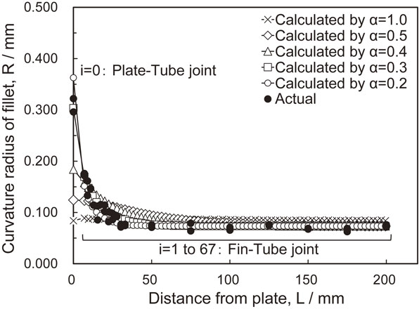
Comparison of actual and numerical model value for the distribution of the curvature radius of the fillet membrane at each joint.
According to these results, it is considered that the flow resistance of the actual flow was larger than that calculated from the numerical model. In the numerical model, the molten filler flow was calculated as the flow between two parallel flat plates because it is assumed that the molten filler flows between the oxide film and the core substrate. In the case of the actual molten filler flow, the path of the molten filler metal was not flat because of the partially destroyed oxide film or the unevenness of the substrate owing to erosion of the core material, thus, a large flow resistance was produced. Therefore, it is considered that the actual flow could be simulated by increasing the flow resistance and using a correction coefficient α for the channel depth d in the numerical model. In addition, the motion of the molten filler in the fillet and the flux among the neglected factors that were shown in the sections 2.2, and the erosion might affect to α. However, the effect of gravity and the solidification shrinkage might not affect to α, because the effect of gravity was sufficiently small from the Bo and the effect of the solidification shrinkage was less than that of the flow resistance.
The curvature radius variations, calculated by the numerical model with increasing temperature, is shown in Fig. 13. These were calculated under the condition of α = 0.3. When the plate and tube temperatures were elevated to 850 K and 851 K, respectively, just above the solidus temperature of the filler alloys AA4343 and AA4045 in 225 s (n = 11250), as shown in Fig. 4, the curvature radii of the fillet at each joint were approximately 0.050 mm each. These fillets were formed by only the tube filler since $K_{i = 0}^{11250}$ was approximately zero for the plate at 850 K and $K_{i \geq 1}^{11250}$ was 0.32 for the tube at 851 K. When the plate and tube temperatures were elevated to 853 K and 852 K in 285 s (n = 14250), and the flow factors were $K_{i = 0}^{14250} = 0.18$ and $K_{i \geq 1}^{14250} = 0.35$, the curvature radius of the fillet at the plate-tube joint increased rapidly. Further, when the plate and tube temperatures were elevated to 859 K in 430 s, and the flow factors were $K_{i = 0}^{21500} = 0.25$ and $K_{i \geq 1}^{21500} = 0.46$, the curvature radius of the fillet at the plate-tube joint reached the maximum value. The growth of the fillet of the plate-tube joint affects the increase in $K_{i = 0}^{n}$ in the plate with increasing temperature. At this temperature, the curvature radii of the fillets at the fin-tube joint within 75 mm from the plate-tube joint are gradually reduced with the distance from the plate-tube joint. It can be seen that the filler of the plate was flowing in the longitudinal direction of the tube. When the temperature was further elevated, the curvature radius of the fillet at the plate-tube joint started to decrease. On the contrary, the curvature radii of the fillet at the fin-tube joint gradually increased for every joint. In particular, the curvature radii of the fillet at fin-tube located within 75 mm from the plate-tube joint were increased significantly with temperature.

Change in the curvature radius distribution of the fillet membrane at each joint during brazing; values were obtained from the numerical model, calculated using α = 0.3.
Since a lot of information can be obtained from the numerical calculations, it is useful to understand the behavior of the molten filler flow during brazing. Furthermore, in this numerical model, it is possible to input various joint shapes, brazing heat cycles, and the contact angle considering the actual brazing atmosphere and flux condition. These approaches might contribute to the optimum placement of the filler metal and the prediction of brazing defects, and eventually to clarify brazing phenomenon in more detail.
However, the present research could not accurately predict the actual molten filler flow because this numerical model simplifies the flow as a uniform flow of incompressible viscous fluid between two parallel plates and the calculations under the assumption stated in section 2.2. Therefore, one of the subjects to improve this numerical model is to reflect upon these neglected factors. To predict the fillet shape and filler flow more accurately, it is necessary to improve the numerical model by experimentally understanding and simulating the flow path of the molten filler, and by measuring the change in the fillet shape with increasing temperature. Furthermore, it is necessary to measure the surface tension, viscosity coefficient, and flow factor more accurately, as these factors change with the brazing cycle, atmosphere, and fluxing. On the other hand, since the fillet shape was determined as a three-dimensional shape and the flow of the molten filler metal was considered as a one-dimensional unsteady flow in this numerical model, its application on more complex shape heat exchangers is quite difficult. Thus, to expand the application of this numerical model, a three-dimensional numerical model of the molten filler flow is necessary for the future.
In this study, a unique numerical analysis method was applied to an automotive aluminum radiator to predict the fillet shape and molten filler flow in the brazing joint and the actual fillet shape of the brazed radiator was compared with the numerical analysis results. Although it was necessary to narrow the flow path in this calculation, the results were consistent with the actual values. This prediction of the fillet shape is very useful in determining the optimum placement of the filler metal, the adequate material choice in the design of the heat exchangers, and the optimization of brazing conditions for the formation of sufficient fillets in the brazed joints.
In order to further increase the accuracy in predicting a fillet shape, it is effective to reflect measurements of the actual flow path of the molten filler, surface tension, viscosity coefficient, and flow factor to the numerical model is effective. On the other hand, given that the fillet shape was determined as a three-dimensional shape and the molten filler flow was ascertained as a one-dimensional unsteady flow in this numerical model, its application on more complex shape heat exchangers is quite difficult. Hence, it will be necessary to enhance the numerical model of the molten filler flow to a three-dimensional model taking into account the neglected factors such as gravity.
The assistance of Mr. Itoh and his colleagues at the Ikeda plant of DENSO Corporation in providing aluminum radiators and advice on brazing technology is gratefully acknowledged.