2. RECT System Using a Linear Amplifier
2.1 Method
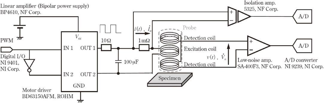
Figure 1 shows an outline of the RECT flaw-detection system. A square-wave signal was generated by a digital-to-analog (D/A) converter (NI Corp., NI 9260, resolution: 24 bit, sampling rate: 51.2 kS/s). The signal was amplified using a high-voltage, high-current, high-speed linear amplifier (bipolar power supply: NF Corp., BP4610), and the exciting coil was driven by a rectangular wave with a frequency of f1 = 10 Hz. A 10 Ω resistor that was sufficiently larger than the impedance of the coil was connected between the bipolar power supply and the excitation coil so that the current amplitude became constant (current amplitude I0 ≅ 2 A). Additionally, a 100 µF capacitor was connected to suppress unnecessary harmonics. Furthermore, a 10 kΩ resistor and a 0.1 µF capacitor were connected to the input of the bipolar power supply, and the ringing that occurred in the D/A converter was suppressed.
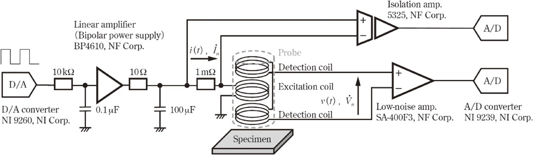
The probe was a mutual induction and differential-type probe with detection coils placed above and below the excitation coil. Each coil had 50 turns, an inner diameter of 20 mm, an outer diameter of 30 mm, and a height of 5 mm. The distance between the coils was 3 mm. The distance (lift-off) between the specimen and detection coil at the lower end was set to 3 mm. The resistance and inductance of the excitation and detection coils were measured using an LCR meter (NF Corp., ZM2371), and the average resistance and inductance were 0.3 Ω and 74 µH, respectively.
The differential voltage v(t) of the detection coil was amplified using an ultra-low noise amplifier (NF Corp., SA-400F3), and the signals were captured using an analog-to-digital (A/D) converter (NI Corp., NI 9239, resolution: 24 bit, sampling rate: 50 kS/s). Simultaneously, the voltage vs(t) of the shunt resistor was captured by the A/D converter, and the exciting current i(t) was obtained. Furthermore, a two-axis automatic stage Sigma Optical Machine, OSMS26-300, was used to measure the exciting current i(t) and differential voltage v(t) of the detection coil when moving the probe in the x- and y-directions at 5 mm intervals on the specimen. Subsequently, a fast Fourier transform of v(t) and i(t) was performed, and the nth harmonic voltage $\dot{V}_{n}(x,y)$ and current $\dot{I}_{n}(x,y)$ were obtained at each measurement point (x, y) (hereafter, the argument (x, y) was omitted to avoid complicating the expression). The dots on the variables indicate that they are in phasor display. The phase of $\dot{V}_{n}$ is based on $\dot{I}_{n}(x,y)$. The control of the D/A converter, recording of signals by the A/D converter, calculation of $\dot{V}_{n}$ and $\dot{I}_{n}(x,y)$, and control of the automatic stage were performed in real time using software developed using LabVIEW (NI Corp.).
There are various methods of inverter excitation,8) but in this study, the most basic rectangular wave excitation was used. For rectangular wave excitation, if the resistance of the excitation circuit is sufficiently large for reactance at the fundamental frequency of the excitation coil, then the current i(t) can be modeled by the periodic function of period T (= 1/f1), as shown in eq. (1).
| \begin{equation}
i(t) =
\begin{cases}
-I_{0} & \text{$\left(-\dfrac{T}{2} \leq t < 0\right)$}\\
I_{0} & \text{$\left(0 \leq t < \dfrac{T}{2}\right)$}
\end{cases}
\end{equation}
| (1) |
where
I0 represents the amplitude of the rectangular wave current. The following equation was obtained by expanding
eq. (1) into a Fourier series:
| \begin{align}
i(t) &= \frac{4I_{0}}{\pi}\sum_{n = 1,3,5,\ldots}\frac{1}{n}\sin n\omega_{1}t \\
&= \frac{4I_{0}}{\pi}\left(\sin \omega_{1}t + \frac{1}{3}\sin 3\omega_{1}t + \frac{1}{5}\sin 5\omega_{1}t + \cdots\right)
\end{align}
| (2) |
where ω
1 denotes the angular frequency of the fundamental wave (ω
1 = 2π
f1). Therefore, the effective value
In of the
nth harmonic current is
$I_{n} = 2\sqrt{2} I_{0}/(n\pi )$ (
n = 1, 3, 5, …), and odd-order harmonics are included in addition to fundamental waves. In this study, the excitation current waveform was used as a rectangular wave to easily interpret the theoretical formulas and experimental results. However, this holds true, even if the excitation voltage waveform is rectangular. One feature of RECT is that the fundamental wave-current amplitude is 4/π (≅ 1.27) times larger than the rectangular wave-current amplitude.
Here, the skin depth δ is $1/\sqrt{\pi \mu \sigma f} $ where the frequency is f, magnetic permeability of the specimen is μ, and conductivity is σ. The skin depth δn for each harmonic of order n is expressed by the following equation.4)
| \begin{equation}
\delta_{n} = \sqrt{\frac{1}{\pi \mu \sigma f}} = \sqrt{\frac{1}{\pi \mu \sigma (nf_{1})}}
\end{equation}
| (3) |
From
eq. (3), the larger the
n, the smaller the δ
n, and only the front surface flaw can be detected.
Because the detection coil is of a differential type, principally, $\dot{V}_{n} = 0$ when there is no specimen. However, when the probe was placed on the specimen, the number of interlinkage magnetic fluxes of the upper and lower detection coils differed. That is, $\dot{V}_{n} = 0$ was not satisfied. Therefore, $\dot{V}_{n}$ was measured when the probe was set in a place without flaws, and the change from that value, $\Delta \dot{V}_{n}$, was obtained. Furthermore, the real part component (in phase with $\dot{I}_{n}$) and imaginary part component (orthogonal with $\dot{I}_{n}$) ($\text{Re}[\Delta \dot{V}_{n}]$, $\text{Im}[\Delta \dot{V}_{n}]$) of $\Delta \dot{V}_{n}$ were obtained. In this study, we focus on $\text{Re}[\Delta \dot{V}_{n}]$, which corresponds to the eddy current component.
Because the induced voltage of the detection coil is proportional to the frequency, $\Delta \dot{V}_{n}$ is normalized with the frequency nf1. Furthermore, the size of $\Delta \dot{V}_{n}$ depends on both the height of the flaw and width in the plane direction. The voltage amplitude of each harmonic is normalized by the voltage amplitude of the fundamental wave, as shown in the following equation:
| \begin{equation}
\Delta S_{n} = \frac{\mathop{\text{Re}}\nolimits[\Delta\dot{V}_{n}]/nf_{1}}{\mathop{\text{Re}}\nolimits[\Delta\dot{V}_{1}]/f_{1}} = \frac{1}{n} \cdot \frac{\mathop{\text{Re}}\nolimits[\Delta\dot{V}_{n}]}{\mathop{\text{Re}}\nolimits[\Delta\dot{V}_{1}]}
\end{equation}
| (4) |
The skin effect is smaller when the flaws were on the front surface than on the back surface. Therefore, the attenuation rate of Δ
Sn in relation to to
n decreases. In contrast, when there is a flaw on the back surface, the attenuation rate of Δ
Sn in relation to
n increased. Furthermore, if there are flaws on the front and back surfaces, both of these characteristics will be exhibited. In other words, the attenuation rate of Δ
Sn in relation to
n is estimated to be in the order of the front surface, both sides, and back surface flaws. Based on this estimation, we attempted to distinguish between the front, back, and double-sided surface flaws using Δ
Sn. The imaging of
$\text{Re}[\Delta \dot{V}_{n}]$ and calculation of Δ
Sn were performed by offline analysis using MATLAB (MathWorks Inc.).
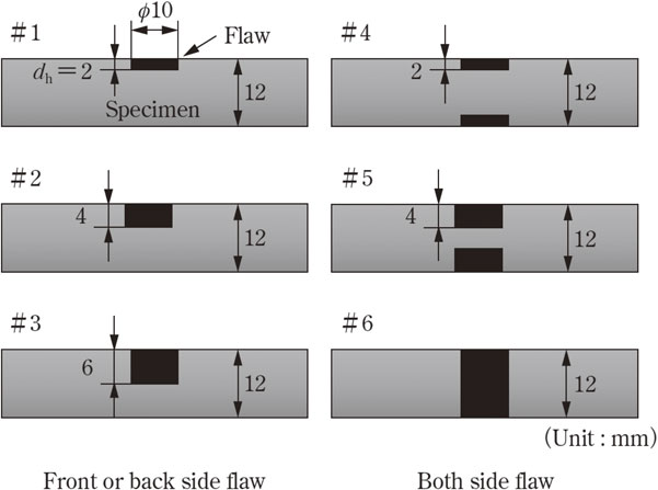
The specimens used in this study are shown in Fig. 2. The specimen was a 300 mm × 300 mm × 12 mm thick aluminum plate with a simulated corrosion flaw in the center and a flat-bottomed drill hole or through hole. The diameter of the flaw was φ10 mm, and the heights dh were 2, 4, and 6 mm. Specimens with flaws on the front, back, and both sides were used (note that dh = 6 mm implies a through-hole in the double-sided flaw). When the relative permeability of aluminum is 1 and the conductivity is 3.57 × 10⁷ S/m, the skin depth is 12 mm, where the frequency is 50 Hz from eq. (3). Thus, the frequency of the excitation current was set to 10 Hz, which was sufficiently lower than 50 Hz.
For comparison, in addition to the square wave, $\Delta \dot{V}_{n}$ was measured when excited individually with a sine wave at each harmonic frequency. To match the measurement conditions during the exact angular wave excitation, the amplitude of the exciting current was set to 4I0/nπ according to eq. (2).
2.2 Results and discussion
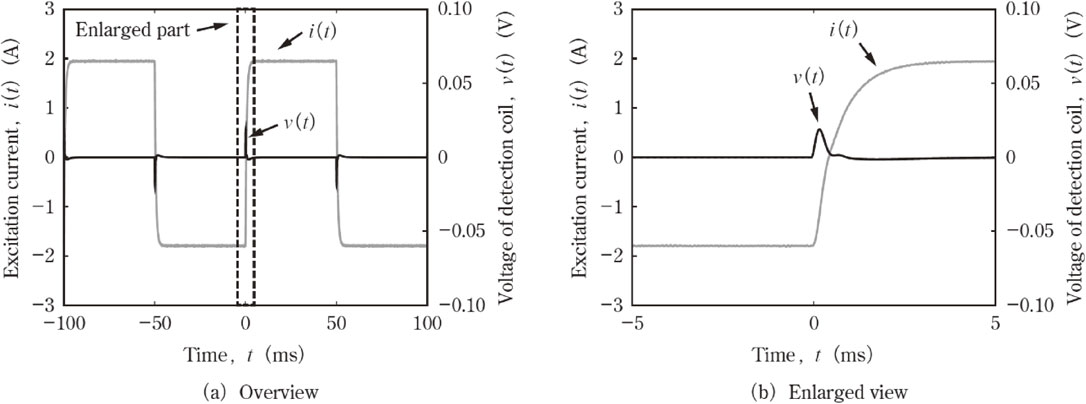
Figure 3 shows the time waveforms of the exciting current i(t) and detected coil voltage v(t) when the probe is placed on the flawless part of the aluminum plate, and a 10 Hz rectangular wave is excited using the RECT system with a linear amplifier as shown in Fig. 1. The time of the rising edge of the current is 0 ms. As shown in Fig. 3, v(t) rises from the rising part of the current, reaches a peak (0.019 V) at t ≅ 0.2 ms, and then asymptotically approaches 0 at t ≅ 0.5 ms.
Figure 4 shows the amplitude spectra of the excitation current and the voltage of the detection coil (resolution: 1 Hz). As shown in the figure, only the fundamental wave and odd-order harmonics appeared for the excitation current. Furthermore, only the fundamental wave and odd-order harmonics appeared in the voltage of the detection coil.
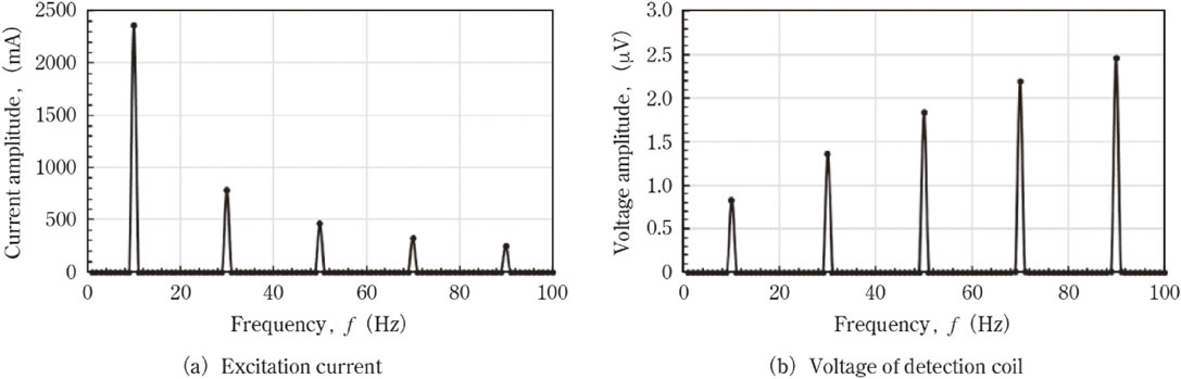
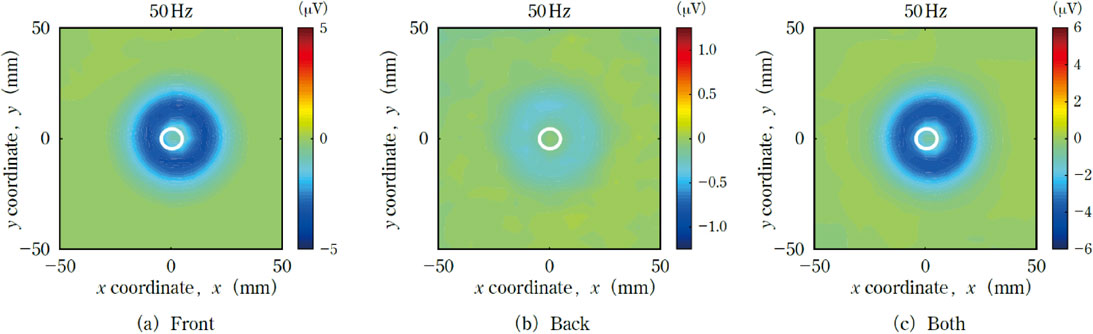
Figure 5 shows the contour diagram of the flaw signal ($\text{Re}[\Delta \dot{V}_{1}]$) of the real part of the fundamental wave of the specimen with a flaw height dh = 4 mm. As shown in the figure, the flaw signal appeared clearly circled at the position of the flaw in the cases of the front, back, and double-sided surface flaws. However, compared with the results for the front surface flaw (Fig. 5(a)) and double-sided flaws (Fig. 5(c)), the signal change was small in the case of the back surface flaw (Fig. 5(b)). This was from the influence of the skin effect and the far position of the flaw. Additionally, the signal change was slightly larger in the case of double-sided flaws than that in the case of front surface flaws. This was because, in the case of double-sided flaws (Fig. 5(c)), both the front (Fig. 5(a)) and back surface flaw signals (Fig. 5(b)) were added. However, the result shown in Fig. 5(c) cannot be immediately regarded as a double-sided flaw by comparing it with that shown in Figs. 5(a) and 5(c). This is because the same result appears when the surface flaws become deeper.
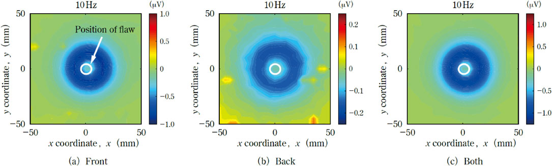
Figure 6 shows the flaw signal ($\text{Re}[\Delta \dot{V}_{5}]$) of the real part of the fifth harmonic under the same conditions. The scale of each color bar is five times larger than that in Fig. 5. In the case of the front surface flaws and double-sided flaws, the flaw signal remained clear; however, the flaws on the back surface were smaller. This was because the harmonic component had a high frequency and the skin effect became stronger.
In Fig. 7, a contour diagram of the flaw signal ($\text{Re}[\Delta \dot{V}_{1}]$) of the real part of the specimen with a flaw height dh = 4 mm when excited by the sinusoidal current corresponding to each harmonic is shown. The same results as those shown in Figs. 5 and 6 were obtained, confirming that multi-frequency testing could be performed using rectangular wave excitation.
Figure 8 shows the relationship between the flaw signal (the average value of the values at the location where the flaw signal appears is circled) and the frequency of each harmonic. Figure 8(a) shows the relationship between the frequency standardization of the flaw signal in the real part ($\text{Re}[\Delta \dot{V}_{n}]/nf_{1}$) and the frequency. Figure 8(b) shows the result of the relationship between the flaw signal (ΔSn) standardized by eq. (4), and the frequency.
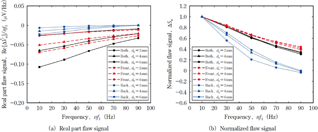
First, the results shown in Fig. 8(a) (plots with ■) indicate that when the height of the flaw was dh = 6 mm with flaws on both sides, front surface, and back surface, the absolute value of the flaw signal was large for the double-sided flaws, small in the order of the front and back surface flaws, and decreased as the frequency increased. Furthermore, the relation holds when dh = 4 and 2 (plotted with ▲ and ●, respectively). Additionally, when the frequency was high, the result in the case of the double-sided flaws was closer to that in the case of surface flaws owing to the skin effect.
Next, the results shown in Fig. 8(b) (plots in black, red, and blue) indicate that with flaws on both sides, front surface, and back surface, in the frequency range of 30 to 100 Hz (approximately 50 Hz, which is the frequency at which the skin depth is approximately half the plate thickness) and at any height of the flaw, the flaw signal decreases in the order of the front surface flaws, double-sided flaws, and back surface flaws. As mentioned in Section 2.1, this is because the signal of the back surface flaws rapidly attenuated with an increase in the frequency owing to the skin effect, such that the attenuation factor of ΔSn in relation to n was larger in the case of the backside flaws than in the case of the front side flaws. Both of these characteristics were observed in the case of the double-sided flaws. Thus, double-sided, front surface, and back surface flaws can be distinguished based on the attenuation of the signal.
The phase of the eddy current for each harmonic of order n at depth x is expressed by the following equation.4)
| \begin{equation}
\theta_{n} = -\frac{x}{\delta_{n}}
\end{equation}
| (5) |
From
eq. (5), because the phase of the eddy current was linearly delayed owing to the skin effect, the phase change increased with the frequency. Hence, a flaw signal due to the eddy current appeared in both the real and imaginary component parts. Therefore, in the back surface corrosion flaw, the sign of the real component is inverted.
Evidently, double-sided, front surface, and back surface flaws can be distinguished based on the attenuation of the signal. Therefore, we considered a simple identification method that uses this feature. For example, consider the 90 Hz signal in Fig. 8(b). The average value of the lower limit of the surface flaw signal (0.390) and upper limit of the double-sided flaw signal (0.352) was 0.371, and the average value of the lower limit of the double-sided flaw signal (0.289) and upper limit of the backside flaw signal (−0.018) was 0.1355. Therefore, double-sided, front, and back surface flaws can be distinguished using these values as determination boundaries.
In this study, the front- and/or back-surface flaws were classified using the aforementioned method because dh did not exceed 6 mm.
3. RECT System Using an Inverter
3.1 Method
Figure 9 shows an outline of the RECT system that uses a motor driver IC as an inverter. A 10 Hz square wave signal (digital waveform) was generated by a digital I/O (NI Corp., NI 9401, 20 MHz (in the case of two output channels)) and input to the motor driver IC (ROHM, BD63150AFM). The motor driver had a full-bridge circuit configuration;8) therefore, bipolar output was possible. By supplying 20 V to the motor driver with the aforementioned bipolar power supply, an exciting current with a rectangular wave of amplitude I0 = 2 A and frequency of f1 = 10 Hz was generated in the excitation coil. A bipolar power supply was used because the power supply device mentioned in Chapter 2 was used. Because neither polarity was required, the system could be further simplified using a unipolar power supply.
3.2 Results and discussion
Figure 10 shows the time waveforms of the exciting current i(t) and detection coil voltage v(t) when a 10 Hz rectangular wave is excited using a RECT system with an inverter, as shown in Fig. 9. The time of the rising edge of the current is 0 ms. As shown in Fig. 10, the current waveform rises sharply, overshot (or undershot), and then converges to a constant current value while oscillating after approximately 100 ms. Thus, the outline is different from that of i(t) (Fig. 3) when excited by a linear amplifier. Therefore, the outline of v(t) also changes, and v(t) rises from the rising part of the current, reaches a peak (0.093 V) at t ≅ 0.1 ms, and then asymptotically approaches 0 at t ≅ 1 ms while oscillating. The signal change was steep in the inverter circuit shown in Fig. 9 because of the absence of a circuit corresponding to the low-pass filter in the input section of the bipolar power supply, as shown in Fig. 1. Additionally, unlike a linear amplifier, this inverter circuit does not have negative feedback, and therefore, a large overshoot occurs.

Figure 11 shows the relationship between the flaw signal and frequency of each harmonic in the case of the inverter excitation. As shown in Fig. 8(b), the flaw signal decreases in the order of front surface flaws, double-sided flaws, and back surface flaws. Therefore, the front and/or back surface flaws can be easily classified using the same method described in Chapter 2, even if the inverter is excited. As shown in Fig. 10, the excitation current waveform differs from that of the excitation by the linear amplifier, such as the overshoot in the case of inverter excitation. However, this component corresponds to the high-frequency component, and almost no effect appears in the band below 100 Hz, which was the target of this study. Thus, the same flaw detection results using the RECT with the linear amplifier were obtained using the RECT with the inverter. Therefore, the flaws of non-magnetic metal materials on the front, back, and double-sided surfaces can be classified by RECT, which is a simple, compact, and lightweight system that uses an inverter.

In a broad sense, RECT can be considered as a type of pulsed ECT (PECT)9–11) that has been widely used. This study differs from general PECT in that the excitation is not instantaneous but is performed at all times, and the exciting magnetic field (current) is bipolar. Similar results are expected even if there is a period when the excitation current is 0 and even if a unipolar field is used instead of a bipolar one. Although the SN ratio and distribution of the frequency components change, similar results are expected. Hence, the knowledge obtained by PECT can be applied to RECT.