Prediction of Dissolution Data Integrated in Tablet Database Using Four-Layered Artificial Neural Networks

Abstract

A large number of dissolution data were measured and integrated into a previously constructed tablet database composed of 14 kinds of compounds as model active pharmaceutical ingredients (APIs) with contents ranging from 10 to 80%. The database has contained physicochemical and powder properties of APIs, together with basic physical attributes of tablets such as the tensile strength and the disintegration time. In order to enhance the value of this database, drug dissolution data are essential to improving key information for designing tablet formulations. A four-layered artificial neural network (4LNN), newly implemented in commercially available software, was employed to predict dissolution data from physicochemical and powder properties of APIs. Our results showed that an excellent model for the prediction of dissolution data was achieved with 4LNN method. The function of 4LNN was appreciably better than that of conventional three-layered model, despite both models adopting the same number of nodes and algorithms for activation functions. Furthermore, linear regression models resulted in poor prediction of dissolution data.

Tablets are one of the most common dosage forms among various pharmaceutical products. Since tablets are produced with many formulation factors such as various excipients and process variables, the relationships between formulation factors and attributes of tablet quality are often complicated. The effects of formulation factors can be substantially modulated by changes in the physicochemical nature of the active pharmaceutical ingredients (APIs). A tablet database would provide the basis for meaningful investigations using reliable candidate formulations, which can be undertaken at the very beginning of the development process. In a previous study,¹⁾ we created a tablet database that included 14 kinds of APIs: acetaminophen, antipyrine, aspirin, ascorbic acid, chloramphenicol, ethenzamide, flufenamic acid, griseofulvin, isoniazid, ketoprofen, mefenamic acid, sulfisoxazole, sulfamonomethoxine and theophylline. Tablets containing 10, 20, 30, 40, 50, 60, 70 and 80% in content of each API were prepared (112 different tablets in total). The tensile strength and disintegration time were measured as basic physical characteristics. Although the scale of the database is not yet sufficient, in a previous study, we found that the nature of API molecules and their powder properties could accurately predict basic physical characteristics, demonstrating the useful application of this database. In addition to the basic characteristics of the tablets, the dissolution rate of APIs is another important factor to consider, as is in partly related to bioavailability.²⁾

Recently, artificial intelligence (AI) has been an emerging theme in the science of complex system, particularly, deep learning^3–5) and sparse modeling^6,7) are increasingly becoming the focus of AI researches. Robust findings using these methods are often reported in the field of image analysis.^3,7,8) Also, commercially available software employing novel AI techniques are continuously being developed, implemented, and updated. In this study, we measured the 112 types of tablets, and aimed to quantitatively predict dissolution data using a combination of physicochemical and powder properties of APIs. For this purpose, we employed four-layered artificial neural network (4LNN),⁹⁾ a machine leaning technique that has recently been implemented in commercially available statistical software. Prediction ability of 4LNN was compared with the conventional three-layered model (3LNN) and classical linear regression equations.

Experimental

Materials

Acetaminophen, flufenamic acid and isoniazid were obtained from Tokyo Kasei Kogyo (Tokyo, Japan). Antipyrine, aspirin, ascorbic acid, chloramphenicol, ethenzamide, griseofulvin, ketoprofen, mefenamic acid, sulfamonomethoxine, theophylline and magnesium stearate (MgSt) were obtained from Wako Pure Chemical Industries, Ltd. (Osaka, Japan). Sulfisoxazole was obtained from Sigma-Aldrich (Tokyo, Japan). Microcrystalline cellulose (Ceolus^® PH-101) was obtained from Asahi Kasei Chemicals (Tokyo, Japan). Lactose (200-mesh grade) was obtained from DMV International (Veghel, the Netherlands). Cornstarch was obtained from Nihon Shokuhin Kako (Tokyo, Japan). Low-substituted hydroxypropyl cellulose (L-HPC^® LH21) was obtained from Shin-Etsu Chemical (Tokyo, Japan). All other chemicals were of reagent grade.

Preparation of Tablets

The preparation methods for tablets containing each API were fully described in detail in the previous paper.¹⁾ Briefly, the ingredients were accurately weighed according to the designated formulations, which were previously optimized in the placebo tablet formulation with acceptable tensile strength and disintegration time. All ingredients, except MgSt, were blended in a polyethylene bag for 2 min. The appropriate amount (0.5%) of MgSt was then added to the mixture and mixed for 1 min. The mixed powder was compressed at 8 kN into a round faced tablet, 8 mm in diameter and 12 mm in curvature radius, using a HANDTAB 100 hydraulic press (Ichihashi-Seiki Company, Ltd., Kyoto, Japan).

Drug Dissolution

According to the Japanese Pharmacopoeia XVII (JP XVII), dissolution test No. 2 (paddle method) for each tablet was conducted at 37±0.5°C with a paddle rotation speed of 50 rpm using 900 mL phosphate buffered saline (pH 7.4) as the dissolution medium. A dissolution tester (NTR 6400ATR, Toyama Sangyo, Co., Ltd., Osaka, Japan) with an auto-sampler (SAS-6000, Toyama Sangyo, Co., Ltd.) was used. Dissolved rates (%) of the APIs at 5, 10, 15, 30 and 60 min (D₅, D₁₀, D₁₅, D₃₀ and D₆₀) in dissolution media were determined using a UV spectrophotometer (V-650, JASCO Corp., Tokyo, Japan). The D₅, D₁₀, D₁₅, D₃₀ and D₆₀ values were analyzed as output variables in the 4LNN model. The mean values of three determinations were used as the dissolution data analysis.

Physicochemical Property and Powder Property

The physicochemical property and powder property values measured in the previous paper¹⁾ were used as causal factors for predicting the dissolution data of the APIs. That is, the melting point (mp, °C), the solubility in water at 37°C (C_s, mg/L), the specific surface area (S_w, cm²/g), the mean particle diameter (d₅₀, µm) and the size distribution (R_w defined by (d₉₀−d₁₀)/d₅₀, where d₁₀ and d₉₀ are the particle diameters at 10 and 90%, respectively) of each API. These values and the API quantity (Q, %) were used as causal input variables.

Neural Network Architecture and Data Analysis

The commercially available statistical software, the JMP Pro 13 (SAS Institute Japan, Co., Ltd., Tokyo, Japan) was employed for the data analysis. 4LNN is composed of 4 layers: 1 input, 2 hidden, and 1 output. Each hidden layer contains nodes, with the nodes in the adjacent layers mutually linked with relevant weights. The functions applied at the nodes of each layer are referred to as activation functions. The hyperbolic tangent (tanH), linear combination (Linear), and Gaussian function (Gauss) were used as activation functions in each node. Although there are an infinite number of artificial neural network (ANN) structures, we investigated models 6/1/1/5 to 6/3/3/5. The 6/1/1/5 model was composed of 6 causal factors in the input, 1 node in the 1st and 2nd hidden, and 5 responses in the output layers. The 6/3/3/5 model was composed of 6 causal factors in the input, 3 nodes in the 1st and 2nd hidden, and 5 responses in the output layers. In total, 361 sets of 4LNN structures were conducted with different combinations of the activation function (tanH, Linear, and Gauss). A “boosting” function was implemented in JMP Pro 13, in order to build a large additive neural network model through fitting sequences of smaller models. Although the boosting function allows quicker identification of the most optimal network model, we could not cover the entire conceivable combinations of networks. Consequently we investigated overall combinations from the 6/1/1/5 to 6/3/3/5 models (361 sets). With regard to validation, the “k-fold” function implemented in the software, was employed. This method divides the original data into k subsets, and each subset, in turn, is used to validate the fit of the model on the rest of the data, fitting a total of k models. The model with the best validation statistic was chosen as the optimal one. This is the best method for fitting small data sets, as it makes efficient use of limited amounts of data. In this study, we employed k=5 (i.e., 80% of training and 20% of validation). The training and validation data were successively repeated 5 times with changing datasets. Using different initial weights of links given at random, 100 iterations of training were conducted. Subsequently, the total number of 4LNN trained was 902500 (5×361×5×100: 5 times repetition of trials, 361 combinations of nodes in hidden layers, 5-fold validation, and 100 iterations of different initial weights). Physicochemical and powder properties of the APIs as input factors were previously normalized. Robust fitting, using least absolute deviations rather than least squares, was used for the training process. To mitigate the tendency of 4LNN to over-fit the data, a squared method was chosen as the penalty function. JMP Pro 13 was also applied to performing the data analysis using conventional 3LNN, multiple regression analysis, ANOVA, and calculating other statistical quantities.

Results and Discussion

Single Correlation Analysis

The correlation matrix is summarized in Table 1. A fairly good correlation between dissolution data was observed in the early dissolution stage (r=0.963 for D₅ vs. D₁₀), and gradually weakened with the passage of dissolution time. Similarly, in the final dissolution stage, a strong correlation between D₃₀ and D₆₀ (r=0.971) was observed, but weakened with the passage of dissolution time. Solubility of the APIs (log C_s) had the greatest effect on the dissolution data. Though in the initial dissolution stage, the effect of log C_s was apparent (r=0.617 for D₅), it gradually lessened with time (r=0.584 for D₁₀, r=0.547 for D₁₅, r=0.468 for D₃₀, and r=0.402 for D₆₀). Effects of the other physicochemical or powder properties on the dissolution data were weaker compared with log C_s.

Table 1. Correlation Matrix of Physicochemical and Powder Properties vs. Dissolution Data

	mp	log Cs	log Sw	d50	Rw	Q	D5	D10	D15	D30
log Cs	−0.251
log Sw	0.272	−0.455
d50	−0.438	0.428	−0.628
Rw	−0.358	−0.130	−0.028	−0.338
Q	0	0	0	0	0
D5	−0.091	0.617	−0.206	0.312	−0.227	−0.312
D10	−0.153	0.584	−0.236	0.338	−0.163	−0.261	0.963
D15	−0.236	0.547	−0.263	0.367	−0.069	−0.195	0.894	0.964
D30	−0.303	0.468	−0.302	0.380	0.048	−0.148	0.769	0.874	0.950
D60	−0.332	0.402	−0.337	0.376	0.137	−0.137	0.660	0.778	0.872	0.971

Multiple Regression Analysis

Multiple regression analysis was applied to the dissolution data, D₅ to D₆₀. Regression models were optimized using the stepwise variable forward selection method, which gave the smallest values of the Bayesian Information Criterion (BIC).¹⁰⁾ The optimal equations are as follows:   

(1)

  

(2)

  

(3)

  

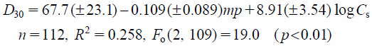(4)

  

(5)

where n is the number of samples, R² is the coefficient of determination, F_o is the observed variance ratio, and the number in parentheses is the 95% confidence interval of regression coefficients. In the optimal regression equations for D₅, D₁₀ and D₁₅, the log C_s and Q values were highly significant and were essential for predicting the early dissolution stage of the APIs. Greater log C_s and smaller Q values resulted in optimal dissolution rates (Eqs. 1–3). Q values likely functioned as phase separation factors since the single effect on the dissolution data was obscure (Table 1). Alternatively, factors such as d₅₀, mp and R_w were chosen instead of Q values in the equations for predicting the last dissolution stage (D₃₀ and D₆₀). The log C_s value was consistently found in the equations for D₅ to D₆₀. ANOVA results suggested that all regression equations were highly significant (p<0.01), but their prediction ability was considerably poor, with the lowest prediction ability observed in the last dissolution stage. The effect of R_w was negative in the initial (Eq. 1), but positive in the last stage (Eq. 5). The d₅₀ values acted as a positive factor in the last dissolution stage (Eqs. 4, 5), indicating that greater dissolution may be obtained with larger API particle sizes. These results are inconsistent with well-known physicochemical findings,^11,12) suggesting uncertainty with Eqs. 4 and 5. The mp negatively affected the last dissolution stage (Eqs. 4, 5). With lower mp associated with weaker API crystal lattices.¹³⁾ Though this factor was not significant in Eq. 5, it was retained in the stepwise regression method.

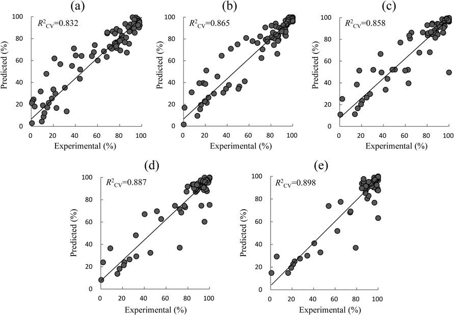
4LNN Analysis

Figure 1 shows the final optimal structure of 4LNN selected from 361 different 4LNNs. With regard to the activation functions, 2 Linear and 1 Gauss in the 1st hidden layer, and 1 tanH, 1 Linear and 1 Gauss in the 2nd hidden layer were selected in the optimal 4LNN. Cross-validation results are summarized in Table 2. Figure 2 shows relationships between the experimental dissolution data and 5-fold cross-validation results (Trial #5 in Table 2). The R²_CV values denote R² for each of the 5-fold cross-validation results of resampling the dissolution data into 80% training and 20% validation, with the resampling process sequentially repeated 5 times. Prediction ability of the 4LNN was superior to that of linear regression equations, though there were variations in the R²_CV values. Relative standard deviations (RSDs, %) of R²_CV values were less than 5% except in the case of D₆₀, where the RSD was 16%. D₆₀ values were observed to be 95% or greater in 70 samples (62.5% of the total 112 tested). Such small difference may have contributed to the variations in the predicted data of the 4LNN models.

Fig. 1. Optimal Structure of Four-Layered Artificial Neural Network

Table 2. R²_CV Values Obtained from 5-Fold Cross-Validation Using the Optimal 4LNN

Trial	Dissolution data
	D5	D10	D15	D30	D60
1	0.866	0.908	0.890	0.904	0.872
2	0.830	0.873	0.865	0.831	0.642
3	0.794	0.860	0.865	0.849	0.658
4	0.784	0.866	0.915	0.914	0.880
5	0.832	0.865	0.858	0.887	0.898
Mean	0.821	0.874	0.879	0.877	0.790
S.D.	0.033	0.019	0.024	0.036	0.128
RSD (%)	4.02	2.17	2.73	4.10	16.20

Fig. 2. Relationship between Experimental Dissolution Data and Cross-Validated Results with 4LNN (6/3/3/5; Trial #5 in Table 2)

Keys: a; D₅, b; D₁₀, c; D₁₅, d; D₃₀, e; D₆₀.

4LNNs were compared with the conventional 3LNN method, which were composed of 6 causal factors in the input, 6 nodes in the hidden and 5 responses in the output layers (6/6/5). With regard to activation functions, 1 tanH, 3 Linear and 2 Gauss were used. These functions were selected using the optimal 4LNN structure as a reference (1 tanH, 1 Linear and 1 Gauss in the 1st hidden layer; 2 Liner and 1 Gauss in the 2nd hidden layer, i.e., 1 tanH, 3 Linear and 2 Gauss in total). Results are given in Table 3. The R²_CV values observed with 3LNNs were lower than those of the 4LNNs except in the case of D₁₅. Additionally, the RSD values of the R²_CV were considerably larger than those in the 4LNNs. The number of unknown weights in 3LNN was 66 (6×6+6×5), compared to 42 (6×3+3×3+3×5) in the 4LNN analysis, suggesting that the internal structure of the 3LNN was more complex than the 4LNN. While 3LNN is more advantageous for training the test data, there is a tendency to over-fit, resulting in poor validation.¹⁴⁾ On the contrary, in 4LNN, the 6 causal factors are simplified into 3 nodes in the 1st hidden layer. Properly integrated information will then be transferred to the 3 nodes in the 2nd hidden layer, and finally, the secured outcome is delivered in the output layer. This suggests that deeper hierarchical structures may be better for more robust prediction.^7,15–17) In this study, the number of sample tablets is still less so that prediction in the 4LNN models is limited in the range of this dataset. A wide range of data should be integrated, in order to accomplish universal and comprehensive predictions.

Table 3. R²_CV Values Obtained from 5-Fold Cross-Validation Using the Referential 3LNN

Trial	Dissolution data
	D5	D10	D15	D30	D60
1	0.909	0.971	0.980	0.682	0.362
2	0.800	0.886	0.876	0.582	0.463
3	0.686	0.799	0.829	0.745	0.459
4	0.861	0.970	0.943	0.783	0.555
5	0.800	0.855	0.933	0.967	0.890
Mean	0.811	0.896	0.912	0.752	0.546
S.D.	0.084	0.075	0.060	0.142	0.204
RSD (%)	10.36	8.37	6.58	18.88	37.36

Sensitivity Analysis

The sensitivity of the dissolution data to each physicochemical and powder property of the APIs was analyzed.^18–20) The basic measure of sensitivity is the change in prediction accuracy of 4LNNs following the application of a leave-one-factor-out (LOFO) procedure. First, the R²_CV-LOFO value was estimated by the 5-fold cross-validation using the LOFO data. Then, the sensitivity of the dissolution data to designated factors was defined as:   

(6)

When a factor contributing to the prediction accuracy is removed from the original data, the sensitivity should increase. If the sensitivity index defined by Eq. 6 is positive, the factor is a significant predictor of the dissolution data, thereby allowing for the identification of factors that are significant or insignificant to the dissolution of each API from tablets. Sensitivity was determined by R²_CV-original and R²_CV-LOFO for the mean of 5-trials. Results are summarized in Table 4.

Table 4. Sensitivity of Dissolution Data to Physicochemical and Powder Properties

Dissolution data	Sensitivity (%)
	mp	log Cs	log Sw	d50	Rw	Q
D5	7.33	23.25	1.56	2.53	−2.07	33.59
D10	8.06	12.42	2.12	1.40	0.23	28.92
D15	10.46	6.68	1.91	1.45	−1.37	27.91
D30	2.60	2.68	3.21	2.02	−2.28	11.62
D60	7.30	3.12	1.62	1.27	−11.01	2.37

In the initial dissolution stage (D₅–D₁₅), Q, log C_s and mp values were significant factors. Powder properties such as log S_w and d₅₀ were less effective, and R_w slightly disturbed 4LNN approximations except in the case of D₁₀. It was rather serious in the prediction of D₆₀ (Sensitivity=−11%), and then the 4LNN models without using R_w were trained. As a result, more robust validation was accomplished (Table 5, Fig. 3). Especially, D₆₀ values were exceptionally well predicted. Thus, if variables in this tablet database needed to be restricted, molecular nature of the APIs would take precedence as it was more important for predicting dissolution data than powder properties.

Table 5. R²_CV Values Obtained from 5-Fold Cross-Validation with 4LNN without Using R_w

Trial	Dissolution data
	D5	D10	D15	D30	D60
1	0.863	0.879	0.900	0.905	0.889
2	0.862	0.904	0.914	0.914	0.902
3	0.801	0.829	0.828	0.853	0.860
4	0.863	0.879	0.900	0.905	0.889
5	0.801	0.871	0.915	0.901	0.842
Mean	0.838	0.872	0.891	0.896	0.876
S.D.	0.034	0.027	0.036	0.024	0.025
RSD (%)	4.06	3.10	4.04	2.68	2.85

Fig. 3. Relationship between Experimental Dissolution Data and Cross-Validated Results with 4LNN without Using R_w (5/3/3/5; Trial #5 in Table 5)

Keys: a; D₅, b; D₁₀, c; D₁₅, d; D₃₀, e; D₆₀.

Conclusion

The tablet database, in which dissolution data were implemented, was created in this study. This database was useful in determining reliable formulations with preferable dissolution profiles, as well as more superior basic characteristics including tensile strength and disintegration time. An excellent dissolution prediction model was obtained using 4LNN, which was appreciably better than conventional 3LNN models. Linear regression models resulted in very poor prediction of dissolution data. Further investigations should focus on identifying the effect of appropriate powder properties of APIs.

Acknowledgment

This study was supported by the Japan Society for the Promotion of Science (JSPS) KAKENHI Grant Number JP17K08252. The authors are grateful to Ms. Saori Mitsumoto for her assistance in the experimental works.

Conflict of Interest

The authors declare no conflict of interest.

References

• 1) Onuki Y., Kawai S., Arai H., Maeda J., Takagaki K., Takayama K., J. Pharm. Sci., 101, 2372–2381 (2012).
• 2) Amidon G. L., Lennernäs H., Shah V. P., Crison J. R., Pharm. Res., 12, 413–420 (1995).
• 3) LeCun Y., Bengio Y., Hinton G., Nature (London), 521, 436–444 (2015).
• 4) Huang G., Huang G.-B., Song S., You K., Neural Netw., 61, 32–48 (2015).
• 5) Schmidhuber J., Neural Netw., 61, 85–117 (2015).
• 6) Bruckstein A. M., Donoho D. L., Elad M., SIAM Rev., 51, 34–81 (2009).
• 7) Yang J., Wright J., Huang T. S., Ma Y., IEEE Trans. Image Process., 19, 2861–2873 (2010).
• 8) “Large Scale Visual Recognition Challenge, 2015 (ILSVRC2015).”: ‹http://image-net.org/›
• 9) Ibrić S., Djuriš J., Parojčić J., Djurić Z., Pharmaceutics, 4, 531–550 (2012).
• 10) Tamura Y., Sato T., Ooe M., Ishiguro M., Geophys. J. Int., 104, 507–516 (1991).
• 11) Lindberg N.-O., Lundstedt T., Drug Dev. Ind. Pharm., 20, 2547–2550 (1994).
• 12) Zimper U., Aaltonen J., Krauel-Goellner K., Gordon K. C., Strachan C. J., Rades T., Pharmaceutics, 2, 419–431 (2010).
• 13) Batisai E., Ayamine A., Kilinkissa O. E. Y., Báthori N. B., CrystEngComm, 16, 9992–9998 (2014).
• 14) Hawkins D. M., J. Chem. Inf. Comput. Sci., 44, 1–12 (2004).
• 15) Ma J., Sheridan R. P., Liaw A., Dahl G. E., Svetnik V., J. Chem. Inf. Model., 55, 263–274 (2015).
• 16) Dong W., Zhang L., Shi G., Wu X., IEEE Trans. Image Process., 20, 1838–1857 (2011).
• 17) Yu W., Zhuang F., He Q., Shi Z., Neurocomputing, 149, 308–315 (2015).
• 18) Farabet C., Couprie C., Najman L., LeCun Y., IEEE Trans. Pattern Anal. Mach. Intell., 35, 1915–1929 (2013).
• 19) Olden J. D., Joy M. K., Death R. G., Ecol. Modell., 178, 389–397 (2004).
• 20) Kikuchi S., Takayama K., Int. J. Pharm., 374, 5–11 (2009).