Significance of Data Selection in Deep Learning for Reliable Binding Mode Prediction of Ligands in the Active Site of CYP3A4

Abstract

For rational drug design, it is essential to predict the binding mode of protein–ligand complexes. Although various machine learning-based models have been reported that use convolutional neural networks (deep learning) to predict binding modes from three-dimensional structures, there are few detailed reports on how best to construct and use datasets. Here, we examined how different datasets affected the prediction of the binding mode of CYP3A4 by a three-dimensional neural network when the number of crystal structures for the target protein was limited. We used four different training datasets: one large, general dataset containing various protein complexes and three smaller, more specific datasets containing complexes with CYP3A4-like pockets, complexes with CYP3A4-binding ligands, and complexes with CYP protein family members. We then trained models with different combinations of datasets with or without subsequent fine-tuning and evaluated the binding mode prediction performance of each model. The best receiver operating characteristic (ROC) area under the curve (AUC) model with respect to area under the receiver operating characteristic curve was obtained by training with a combination of the general protein and CYP family datasets. However, the ROC AUC—recall balanced model was obtained by training with this combination of datasets followed by fine-tuning with the CYP3A4-binding ligands dataset. Our results suggest that datasets that balance protein functionality and data size are important for optimizing binding mode prediction performance. In addition, datasets with large median binding pocket sizes may be important for the binding mode prediction specifically of CYP3A4.

Introduction

The field of medicinal chemistry and drug design have undergone revolutionary changes inspired by recent scientific and technological innovations.^1,2) In particular, computational methodologies are frequently used to reduce the cost and improve the hit-rate of experimental verification and guide medicinal chemists in the hit to lead optimization. For rational and efficient structure-based drug design, it is essential to clarify the binding modes of hits and leads with target proteins. Since the late 2000s, rapid docking algorithms, such as Glide³⁾ and DOCK,⁴⁾ that use protein structures have been widely used to predict the binding modes of designed compounds; in such docking algorithms, the various docking poses of a compound are evaluated by using empirical, knowledge-based, and physically inspired scoring functions.^3–9) However, as the number of protein–ligand complexes registered in the Protein Data Bank (PDB) has increased, attention has shifted to the use of faster and more efficient machine learning methods that use the binding features of protein–ligand interactions such as interatomic distance, angle, and solvent-accessible surface area.^10–13)

CYPs are proteins responsible for the majority of phase I drug metabolism. Nearly 80% of drugs in current use or undergoing clinical trial are metabolized by CYPs. Therefore, accurate prediction of the binding mode between drug candidates and CYPs is important for the design of drugs with metabolic stability and few drug–drug interactions originating from CYP inhibition. CYP3A4 is an important CYP that is involved in the metabolism of more than 30% of drugs in current use¹⁴⁾ due to its binding pocket being larger^15,16) and more flexible¹⁷⁾ than that of the other CYPs, which allows it to accommodate various substrates; however, this makes it difficult to use conventional docking algorithms and scores to predict the binding mode between a substrate and CYP3A4.

In machine learning methods for binding mode prediction, protein–ligand interactions are treated as usually one-dimensional descriptors and fingerprints.^18–26) These methods have an accuracy that is comparable with that of conventional docking algorithms; however, there are concerns that the spatial arrangement information of the protein–ligand complex in three-dimensional (3D) space is lost and that some interactions by ring-type ligands, such as dispersion interactions, are not appropriately taken into account.²⁷⁾

Recently, machine learning methods using 3D structure information have been developed.^28–32) The main advantage of 3D structure-based machine learning methods is that they use 3D locations of atomic-level protein–ligand interactions such as the atom-type density of each interacting atom, as well as interactions between target atoms and their surrounding atoms such as ionic bonds, hydrogen bonds, and van der Waals interactions. This makes it possible to evaluate the correctness of the docking pose without losing the spatial arrangement information of the proteins and ligands that are the essence of docking. However, when performing machine learning using a 3D structure in drug discovery, there are many cases where the size of learning data is limited, especially for a new drug target. In these cases, the issue of how to create training dataset is emerged.

Wallach et al. developed the first machine learning model for binding mode prediction, AtomNet, which uses a deep convolutional neural network (CNN) to handle the protein structure as voxel grid.²⁸⁾ In AtomNet, the binding sites of ligands are expressed as cubes with sides of 20 Å arranged in a grid with an interval of 1 Å, and the grid holds values that represent structural features. By hierarchically constructing a deep CNN architecture, AtomNet is able to model the complicated nonlinear phenomena of protein–ligand binding, significantly outperforming conventional docking approaches for a diverse range of benchmark datasets and achieving area under the receiver operating characteristic (ROC) curve values greater than 0.9 for 57.8% of targets in the Dictionary of Useful Decoys, Enhanced database.³³⁾

Ragoza et al. have developed a CNN scoring function similar to AtomNet for 3D representations of protein–ligand interactions.³⁰⁾ In this scoring function, cubes with sides of 24 Å are arranged in grids with an interval of 0.5 Å, and the densities of atom types in smina⁹⁾ are allocated to individual grids. Using this approach afforded scores for both pose prediction and virtual screening that were superior to those obtained with AutoDock Vina.⁸⁾ Hochuli et al. also developed a useful visualization method that decomposes the CNN-based score into individual atomic contributions using Ragoza’s architecture.³⁴⁾ We use their visualization method in the discussion part of this paper.

An additional advantage of using deep neural networks is that trained models using other large data set can be re-purposed as a basis when the training dataset is small. The recent intensive study of the concept of re-training has resulted in the development of concepts such as transfer learning, inductive learning, and multitask learning. For example, pre-training is a transfer learning technique that improves prediction performance for new tasks by utilizing models already trained with related data.³⁵⁾ However, the training performance of deep neural networks, including CNNs, is often strongly affected by training set bias and overfitting, especially when the size of the training dataset is small. To address this issue, we have examined the use of pre-training using a large dataset containing a wide range of ligands to construct general binding mode models applicable to various target proteins without overfitting that are then subsequently fine-tuned to allow the model to take specific features of the target protein into consideration. It should be noted that models constructed with a combination of pre-training and fine-tuning almost always show better performance compared with non-fine-tuned models.^36–38)

As of 2017, only around 30 crystal structures had been reported for CYP3A4; therefore, for pre-training and subsequent fine-tuning of a CNN-based model, the crystal structures of a large number of other proteins similar to CYP3A4 must be prepared. To mitigate this issue, in the present study we used four training datasets of various specificities and sizes. By using these four datasets in various combinations, with or without fine-tuning, we examined how dataset construction and selection for pre-training and fine-tuning affected the accuracy of a neural network model for predicting the docking pose for binding CYP3A4. In addition, we visualized the binding mode features learned by our model.

Experimental

A workflow summarizing from data set preparation to model evaluation is shown in Fig. 1.

Fig. 1. Workflow from Dataset Creation to Model Evaluation

Datasets

Four training datasets and one test dataset were used in this study (Table 1). The largest dataset, the general protein dataset (GP dataset, Table S1), was constructed for the model to learn the general characteristics of protein–ligand complexes. The dataset contained 337 various protein complexes with a binding affinity greater than 10 µM selected from the CSAR-NRC HiQ and CSAR HiQ Update datasets.³⁹⁾ The complexes were selected by following the methods of Ragoza et al.³⁰⁾

Table 1. Summary of the Training and Test Datasets

		Shortened names	Number of complex structures	Number of positive poses	Number of negative poses
Training sets	General protein complexes	GP	337	2338	2807
	Complexes with CYP3A4-like pockets	PL	64	708	2842
	Complexes with CYP3A4-binding ligands	LL	28	157	1174
	CYP family complexes	CF	116	1086	4945
Test set	CYP3A4	—	22	22	693

The second dataset (PL dataset, Table S2) was about 20% the size of the GP dataset and contained 64 complexes of various protein species that contained a CYP3A4-like pocket. This dataset was constructed for the model to learn the features of CYP3A4-like pockets. The dataset was constructed by using the PoSSuM database.⁴⁰⁾ As of September 2014, the PoSSuM database contained 5513691 known and putative binding sites obtained from the PDB.⁴¹⁾ To perform an exhaustive similarity search, each ligand binding site was encoded as a feature vector based on a molecular fingerprinting method.⁴²⁾ Similar pairs of binding site were enumerated by using SketchSort⁴³⁾ in PoSSuM database and searched by using a previously reported ultrafast search method.⁴⁴⁾ Search K⁴⁰⁾ was used to find binding sites similar to known ligand binding sites by using PDB IDs of CYP3A4. To obtain as many complexes as possible, the cosine similarity cut-off parameter was set to the lowest value of 0.77. The covalent ligand complex was deleted. Pocket volume was calculated by Site Finder program in MOE.⁴⁵⁾

The third dataset (LL dataset, Table S3) was about 10% the size of the GP dataset and contained 28 complexes containing a known CYP3A4 ligand. This dataset was constructed for the model to learn the atomic-level features that characterize the binding mode between CYP3A4 and its ligands. This dataset was constructed via chemical ID searches of the PDB database using seventeen known CYP3A4 ligands as queries.

The fourth dataset (CF dataset, Table S4) was about 30% the size of the GP set and contained 116 complexes containing a CYP that had been obtained by PDB search. This dataset was constructed for the model to learn the features common among CYP–ligand interactions.

The test dataset (CYP3A4 dataset, Table S5) was constructed in 2017 at the start of the present study and contained twenty-two CYP3A4 complexes in which the ligands were bound near the heme group. When a complex contained two ligands and both were bound near the heme group (i.e., complexes 4K9T and 4K9U), the ligands were undocked and then redocked individually to provide two different complexes, thus ensuring that none of the data overlapped.

In all cases of dataset creation, we used the docking program in MOE⁴⁵⁾ to generate the ligand docking poses. ‘Ligand’ was specified as the docking site, and all other atoms, except the ligand atoms, were specified as ‘receptor.’ Default values were used for all other settings. Under the parameter setting, all ligands in the crystal structures were redocked. The Alpha Triangle algorithm⁷⁾ was used to place the ligands in the binding site, and the binding energy was scored according to the London ΔG scoring function. The Amber10:EHT force field was used to minimize the docking poses. As in the paper of Ragoza et al.,³⁰⁾ up to 20 poses were outputted for each crystal structure in the GP set. Up to 70 docking poses were outputted from the other four training sets because the amount of data was much smaller than the number of data with the GP set. After docking, we manually fixed inappropriate ligand structures that were in the incorrect protonation state or had an incorrect bond order. The ligand conformations in the crystal structures were added to the datasets so that all of the datasets contained ‘correct poses.’ The reason for this was the fact that it is difficult to obtain the correct pose by docking only when a highly flexible compound binds to a large binding pocket.⁴⁶⁾ For the purposes of training, poses with a heavy-atom root-mean-square deviation (RMSD) less than 2 Å from the crystal pose were tagged as positive (correct) poses, and those with an RMSD greater than 4 Å were tagged as negative (incorrect) poses (Fig. 2). Only the ligand conformations in the complex structures were used as positive poses in the CYP3A4 dataset. The numbers of positive and negative poses in each dataset are shown in Table 1.

Fig. 2. Positive and Negative Docking Pose Examples

Poses with a heavy-atom root-mean-square deviation (RMSD) less than 2 Å from the crystal pose were tagged as positive examples (correct poses), and those with an RMSD greater than 4 Å RMSD were tagged as negative examples (incorrect poses). (Color figure can be accessed in the online version.)

Input Format

Following the methods of Ragoza et al.,³⁰⁾ the atom types of the protein–ligand structures were expressed as values allocated to each grid point and then used as the input for the CNN. The grid used was a 24 ų cube with a resolution of 0.5 Å that was centered on the center of mass of the binding site. There were 34 possible atom types at each point on the 3D grid that corresponded to the density of protein atoms (16 atom types) and ligand atoms (18 atom types). The definitions of the atom types and the formula for calculating atom-type density were the same as those used by Ragoza et al.³⁰⁾ (Table S6 and Fig. S1, respectively).

CNN Architecture

Our CNN models used the optimized model architecture published on GitHub (https://github.com/gnina/models).³⁰⁾ The model has three 3 × 3 × 3 convolution layers each with a rectified linear unit as the activation function (Fig. S2). In the first convolution layer, 34 feature maps are generated. Each convolution layer is followed by a pooling layer in which max pooling with a kernel size of two is used and the dimensions of the maps are halved. After the input has passed through each of the convolution and pooling layers, it continues to a fully connected layer then to a softmax layer as the output layer, which scales the predictions to between zero and one and the sum to one.

Training

The CNN models were defined and trained by using the Caffe deep learning framework⁴⁷⁾ with the MolGridData layer input format.³⁰⁾ All networks of CNN model were trained using stochastic gradient descent to minimize multinomial logistic loss. The model batch size was 10 and the number of iterations was 10000. Following the work of Ragoza et al.,³⁰⁾ the parameters used for all models were as follows: learning rate = 0.01; momentum = 0.9; inverse learning rate decay with power = 1 and gamma = 0.001; and regularization with weight_decay = 0.001 and dropout_ratio = 0.5. Input grids were augmented by randomly rotating and translating the input structures 24 times on-the-fly.

Model Evaluation

The CYP3A4 dataset was designed to test the binding mode prediction of the CNN models trained with the training datasets. Three-fold cross-validation was used for evaluation of the CYP3A4 dataset. To improve prediction accuracy, the complexes in the CYP3A4 dataset were divided into three groups: ritonavir analogue complexes with a similar binding mode, complexes bound near the heme group, and all other complexes. Since all entries in the CYP3A4 dataset have the same amino acid sequence, data decomposition by sequence similarity was not used (Fig. S3).

To evaluate prediction performance from multiple angles, the following indicators were used: area under the ROC curve, recall, and score ranking. The ROC⁴⁸⁾ curve depicts overall classification performance by plotting true-positive rates against false-positive rates. The area under the ROC curve is a performance metric where area under the curve (AUC) = 1 represents a perfect classifier and AUC <0.5 is not better than random selection. Recall was defined as the proportion of experimentally correct poses among the predicted positive poses (CNN score >0.5); the mathematical definition is recall = TP/(TP + FP), where TP and FP are the number of true positives and false positives, respectively. Score ranking is used for correct pose enrichment with regards to CNN score; the enrichment factor is indicated by the sum and average of CNN scores of correct poses included in the topX% when ordered by CNN score.

Fine-Tuning

Fine-tuning is a technique in which a model is further trained using a second, more-specific dataset after the model has been pre-trained with a larger, less-specific dataset. In the present study, the models learned the general features of protein–ligand complexes by pre-training with the GP dataset or a combination of the GP + CF datasets. Fine-tuning was then performed by using one of the CYP-specific datasets (PL, LL, or CF dataset) or their combination. To examine the effectiveness of the pre-training, two fine-tuning schemes were used: (1) classifier (final layer) fine-tuning with all other layer parameters fixed, and (2) all layer fine-tuning (Fig. 3).

Fig. 3. Examples of the Different Training Schemes Used to Construct the Models

(Color figure can be accessed in the online version.)

Visualization

The atoms and fragments in a ligand contributing to a given binding mode prediction were visualized by using the masking algorithm developed by Hochuli et al.³⁴⁾ Masking is a method to evaluate the sensitivity of a model by computing the difference of the predicted output scores between the original input and a masked version of the original input. In the present study, ligand atoms or fragments in a ligand–protein complex were deleted one at a time and the score was calculated. The program we used is available as ‘gninavis’ under an open source license as part of the gnina project (http://github.com/gnina).

Results and Discussion

The results of this study comprise a comparison of the effects of using different combinations of datasets on prediction performance, as assessed by using AUC and recall, a comparison of the effects different fine-tuning schemes and different datasets have on AUC and recall, and the results of a correct pose enrichment analysis with score ranking (topX% and CNN score). From a medicinal chemistry point of view, the detection of experimentally correct poses with a high score and ranking is very important for drug design.

Table 2 shows the prediction performance of the models trained with the GP, PL, LL, and CF datasets or their combination. The CYP3A4 dataset was used to obtain ground truth data. First, the AUC for scoring with the docking program in MOE⁴⁵⁾ was 0.579. It was scored with the optimized crystal structures because there were unstable parts in terms of the molecular force field and these docking scores were excessively deteriorated (AUC 0.127). The AUC for the three-fold cross validation of the CYP3A4 dataset was only 0.540, most likely because the dataset was too small for proper neural network machine learning. The AUCs for the GP, PL, LL, and CF datasets were 0.610, 0.470, 0.745, and 0.647, respectively. Although the model trained with the LL set showed the highest AUC, its recall (0.273) was low. These results suggest that when used individually these datasets do not sufficiently capture the binding mode characteristics of CYP3A4–ligand interactions. When we examined the effects on prediction performance of using various combinations of datasets, the combined datasets tended to show improved AUC values compared with those obtained when the individual datasets were used. The highest AUC (0.831) was obtained by using a combination of the GP and CF datasets, although the recall (0.273) was still low. This suggested that a high AUC can be expected when complementary datasets (i.e., the general protein dataset, GP, and the specific CYP family dataset, CF) are used; thus, the combined GP + CF dataset was used for pre-training in the subsequent analyses.

Table 2. Test Set Performance of Combination of Datasets Based on AUC and Recall. A CNN Score of 0.5 or Higher Was Set as a Positive in Recall Evaluation

Dataset	AUCa)	Recall
CYP3A4 (three-fold cross validation)	0.540	—
GP	0.610	0.136
PL	0.470	0.364
LL	0.745	0.273
CF	0.647	0.182
GP + PL	0.635	0.045
GP + LL	0.617	0.364
GP + CF	0.831	0.273
PL + LL + CF	0.713	0.045
GP + PL + LL + CF	0.781	0.227
Docking score (MOE dock)	0.127b)
	0.579c)	—

a) AUC, area under the curve. b) Scored the crystal structure (positive) as it is. c) Crystal structures (positive) were optimized in the same force field as other docking poses and scored.

From these results so far, we compare the prediction performance between the CNN score and the traditional energy-based score. The CNN score is inferior to the energy-based score when the dataset is small (three-fold cross validation of the CYP3A4). On the other hand, we figure out that the prediction accuracy can be improved by the combination of a suitable dataset by this examination even in such a difficult target like CYP3A4. This point is different from energy-based uniform scoring. In addition, when using the crystal structure as it is when evaluating performance on the energy-based scoring, the issue of the difference in the force field appears prominently in the score value. Compared to the energy-based scoring, the CNN score is robust against minor instability due to force field differences compared to energy-based scores.

Fine-tuning is a powerful means of training a small, biased dataset used together with a large, general dataset for pre-training.^35–38) Table 3 shows the prediction performance obtained after fine-tuning using two of the CYP-specific datasets (i.e., PL and LL datasets). Of the two fine-tuning approaches, classifier fine-tuning provided models with better prediction performance than did all-layer fine-tuning for all of the datasets examined (PL, LL, or PL + LL datasets) with respect to both AUC and recall (e.g., AUC 0.769 vs. 0.829 and recall 0.270 vs. 0.500 in LL dataset). The model with the best prediction performance was pre-training (pre) with the GP + CF set followed by classifier fine-tuning (ft-cl) with the LL dataset, i.e., pre(GP + CF)/ft-cl(LL). However, it should be noted that the prediction performance of this fine-tuned model with regards to AUC and recall was still worse than that of the model constructed using only the GP + CF dataset without fine-tuning.

Table 3. Test Set Performance Comparison of Combination of Datasets and Fine Tuning Based on AUC

Pre-training	Fine tuning
	Dataset	All layers		Classifier
		AUC	Recall	AUC	Recall
GP + CF Area under ROC curve: 0.831 Recall: 0.273	PL	0.677	0.000	0.765	0.182
	LL	0.769	0.270	0.829	0.500
	PL + LL	0.792	0.091	0.808	0.273

AUC, area under the curve; ROC, receiver operating characteristic.

To investigate the differences between the model trained with the GP + CF dataset alone and the model trained with pre(GP + CF)/ft-cl(LL), the two models were evaluated multilaterally by using two additional indices: correct pose enrichment and score value distribution. Correct pose enrichment indicates the percentage of correct poses within the topX%. Score value distribution shows whether the CNN scores of the correct poses were significantly higher than the criteria for positive and negative poses. The GP + CF model and the pre(GP + CF)/ft-cl(LL) model showed comparable correct pose enrichment (Fig. 4, Y-axis). However, in terms of average CNN score, the fine-tuned model showed a score approximately twice as high as that of the non-fine-tuned model. Thus, pre-training followed by fine-tuning markedly enhanced the CNN score of correct poses, which allows for the detection of experimentally correct poses at the significantly high score while the difference of the GP + CF model and the pre(GP + CF)/ft-cl(LL) model is negligible in AUC. Considering the data present above, we consider the pre(GP + CF)/ft-cl (LL) model to be the most practical model.

Fig. 4. Scatter Plot of Percentage of Correct Poses within the topX% versus CNN Score

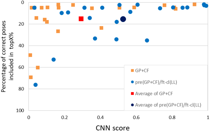
Average percentage of correct poses within the topX%: GP + CF model, 15.1%; pre(GP + CF)/ft-cl(LL) model, 15.2%. Average CNN score: GP + CF model, 0.293; pre(GP + CF)/ft-cl (LL) model, 0.526. (Color figure can be accessed in the online version.)

Overall, the present results indicate that fine-tuning improves binding mode prediction performance as long as an appropriate general dataset is used for pre-training and a target-specific dataset is used for fine-tuning. The GP + CF set greatly improved the AUC and recall for pre-training, and the LL set improved correct pose enrichment with regards to score ranking. To examine these findings further, we conducted a detailed analysis of the datasets with respect to protein classification and pocket size.

To examine why the combined GP + CF dataset was better than the GP dataset for pre-training, we examined the protein composition of the datasets with respect to the proportion of proteins they contained that were classified in the PDB as an oxidoreductase, which is the classification for CYP3A4⁴⁹⁾ (Fig. 5). Because the CF set contained mainly CYPs, 89% of the proteins in that dataset were oxidoreductases. In contrast, only 4% of the proteins in the GP dataset were oxidoreductases. The proportion of oxidoreductases was increased to 25% when the GP and CF datasets were combined, and this proportion was much higher than that of the GP + LL dataset (4%) and the GP + PL dataset (7%). Protein families are groups of proteins that share a common evolutionary origin, which is often reflected in their similar functions and structures. It is likely that the function of a protein is more closely related to the structural similarity around the active site rather than the actual amino acid sequence.⁴²⁾ Thus, it is possible that PDB classification rather than sequence-based family classification is more important for binding mode prediction.

Fig. 5. Percentage of Proteins in Each Dataset That Are Classified in the Protein Data Bank as an Oxidoreductase, the Classfication to Which CYP3A4 Belongs

(Color figure can be accessed in the online version.)

Figure 6 shows a visualization of the change in CNN score for the CYP3A4 pocket of three ligand poses of crystal structure (5VCE, 4D75, 4K9T) when the CF dataset is added to the GP data, as obtained by using a masking algorithm. The figure shows that when the CF dataset is added to the GP dataset, the atoms near the heme group contribute a lot more to the CNN score.

Fig. 6. Visualization of the Change in CNN Score for the CYP3A4 Pocket When the CF Dataset Is Added to the GP Dataset

Three ligand poses of crystal structure are shown. Blue, large increase; green, small increase; silver, unchanged. (Color figure can be accessed in the online version.)

Next, we examined why the LL dataset was better than the PL dataset for fine-tuning. Here, it should be noted that the percentage of oxidoreductases in the dataset containing complexes with CYP3A4-like pockets (PL dataset, 25%) was higher than that in the dataset containing complexes with CYP3A4-binding ligands (LL dataset, 11%). This implies that the lack of improvement in binding mode prediction after fine-tuning with the PL set was a result of factors other than protein classification. An important characteristic of the CYP3A4 dataset is that its median pocket volume (around 1500 ų) was almost twice as large as that of the GP, PL, and CF datasets (Fig. 7). This large median pocket size might be important for binding mode prediction. Although the PL set was designed to include complexes with pocket shapes similar to CYP3A4, the pocket volume range was very similar to those of the GP and CF datasets. In contrast, the pocket volume of the LL set was much larger, almost fully covering the ranges of the other datasets. This suggests that pre-training with the highly complementary GP and CF datasets followed by fine-tuning with the LL dataset captured both the general and specific features of the protein–ligand interactions of CYP3A4.

Fig. 7. Comparison of Pocket Sizes of the Proteins in the Training and Test Datasets

The lines in the box plot represent the minimum, the lower quartile or first quartile, the median, the upper quartile, and the maximum from the left.

Conclusion

Here, we examined how combining datasets of different sizes and specificities and conducting fine-tuning affected the binding mode prediction of a CNN model when the number of protein–ligand complex crystal structures related to the target protein was limited. CYP3A4 was used as the target protein. When we examined the effects of combining datasets, the model trained with the combination of the general dataset containing various protein complexes (GP dataset) and the target-specific dataset containing complexes with CYP protein family members (CF dataset) showed the best area under the ROC curve. This suggested that a dataset well-balanced with respect to protein functionality and data size is important to optimize prediction performance. Pre-training with the combined GP + CF dataset followed by fine-tuning with the dataset containing complexes with CYP3A4-binding ligands (LL dataset) provided a high enrichment score with regards to CNN score ranking and area under the ROC curve. This suggests that a dataset with a large median binding pocket size may be important for the binding mode prediction of CYP3A4.

Future studies are needed to confirm the applicability of the results of the present case study to other target proteins, and improvements of the 3D CNN network structures, descriptors, and fingerprints of interaction which essentially affect the spatial arrangement of ligand and protein are needed. In the field of drug discovery, structural information on proteins of interest is often sparse or biased. For effective drug design, accurate pose prediction models are needed. We believe that neural networks will be a promising approach to address this need once appropriate training dataset design strategies are developed.

Acknowledgments

The 3D-CNN model used in this study is a deliverable commissioned from the Foundation for Biomedical Research and Innovation at Kobe, Kobe, Japan to Mizuho Information & Research Institute, Inc., Tokyo, Japan. This research used computational resources maintained by RIKEN, Yokohama and Kobe, Japan. We thank Mr. Zhang Yuhui of the Konagaya Laboratory, Tokyo Institute of Technology, Kanagawa, Japan, for his support with the model pre-training.

Conflict of Interest

Atsuko Sato is an employee of Kyowa Kirin Co., Ltd., Shizuoka, Japan. Naoki Tanimura is an employee of Mizuho Information & Research Institute, Inc., Tokyo, Japan.

Supplementary Materials

The online version of this article contains supplementary materials.

References

• 1) Panteleev J., Gao H., Jia L., Bioorg. Med. Chem. Lett., 28, 2807–2815 (2018).
• 2) Smith J. S., Roitberg A. E., Isayev O., ACS Med. Chem. Lett., 9, 1065–1069 (2018).
• 3) Friesner R. A., Banks J. L., Murphy R. B., Halgren T. A., Klicic J. J., Mainz D. T., Repasky M. P., Knoll E. H., Shelley M., Perry J. K., Shaw D. E., Francis P., Shenkin P. S., J. Med. Chem., 47, 1739–1749 (2004).
• 4) Allen W. J., Balius T. E., Mukherjee S., Brozell S. R., Moustakas D. T., Lang P. T., Case D. A., Kuntz I. D., Rizzo R. C., J. Comput. Chem., 36, 1132–1156 (2015).
• 5) Böhm H. J., J. Comput. Aided Mol. Des., 8, 243–256 (1994).
• 6) Eldridge M. D., Murray C. W., Auton T. R., Paolini G. V., Mee R. P., J. Comput. Aided Mol. Des., 11, 425–445 (1997).
• 7) Corbeil C. R., Williams C. I., Labute P., J. Comput. Aided Mol. Des., 26, 775–786 (2012).
• 8) Trott O., Olson A. J., J. Comput. Chem., 31, 455–461 (2010).
• 9) Koes D. R., Baumgartner M. P., Camacho C. J., J. Chem. Inf. Model., 53, 1893–1904 (2013).
• 10) Ballester P. J., Mitchell J. B. O., Bioinformatics, 26, 1169–1175 (2010).
• 11) Muegge I., Martin Y. C., J. Med. Chem., 42, 791–804 (1999).
• 12) Gohlke H., Hendlich M., Klebe G., J. Mol. Biol., 295, 337–356 (2000).
• 13) Zhou H., Skolnick J., Biophys. J., 101, 2043–2052 (2011).
• 14) Zanger U. M., Schwab M., Pharmacol. Ther., 138, 103–141 (2013).
• 15) Zaretzki J., Rydberg P., Bergeron C., Bennett K. P., Olsen L., Breneman C. M., J. Chem. Inf. Model., 52, 1637–1659 (2012).
• 16) Kirchmair J., Göller A. H., Lang D., Kunze J., Testa B., Wilson I. D., Glen R. C., Schneider G., Nat. Rev. Drug Discov., 14, 387–404 (2015).
• 17) Skopalík J., Anzenbacher P., Otyepka M., J. Phys. Chem. B, 112, 8165–8173 (2008).
• 18) Ain Q. U., Aleksandrova A., Roessler F. D., Ballester P. J., Wiley Interdiscip. Rev. Comput. Mol. Sci., 5, 405–424 (2015).
• 19) Durrant J. D., McCammon J. A., J. Chem. Inf. Model., 50, 1865–1871 (2010).
• 20) Deng W., Breneman C., Embrechts M. J., J. Chem. Inf. Comput. Sci., 44, 699–703 (2004).
• 21) Velec H. F. G., Gohlke H., Klebe G., J. Med. Chem., 48, 6296–6303 (2005).
• 22) Amini A., Shrimpton P. J., Muggleton S. H., Sternberg M. J. E., Proteins Struct. Funct. Bioinforma., 69, 823–831 (2007).
• 23) Sato T., Honma T., Yokoyama S., J. Chem. Inf. Model., 50, 170–185 (2010).
• 24) Kinnings S. L., Liu N., Tonge P. J., Jackson R. M., Xie L., Bourne P. E., J. Chem. Inf. Model., 51, 408–419 (2011).
• 25) Li L., Khanna M., Jo I., Wang F., Ashpole N. M., Hudmon A., Meroueh S. O., J. Chem. Inf. Model., 51, 755–759 (2011).
• 26) Ashtawy H. M., Mahapatra N. R., BMC Bioinformatics, 16 (Suppl. 6), S3 (2015).
• 27) Gabel J., Desaphy J., Rognan D., J. Chem. Inf. Model., 54, 2807–2815 (2014).
• 28) Wallach I., Dzamba M., Heifets A., ArXiv151002855 Cs (2015).
• 29) Gomes J., Ramsundar B., Feinberg E. N., Pande V. S., ArXiv170310603 Cs (2017).
• 30) Ragoza M., Hochuli J., Idrobo E., Sunseri J., Koes D. R., J. Chem. Inf. Model., 57, 942–957 (2017).
• 31) Imrie F., Bradley A. R., van der Schaar M., Deane C. M., J. Chem. Inf. Model., 58, 2319–2330 (2018).
• 32) Jiménez J., Škalič M., Martínez-Rosell G., De Fabritiis G., J. Chem. Inf. Model., 58, 287–296 (2018).
• 33) Mysinger M. M., Carchia M., Irwin J. J., Shoichet B. K., J. Med. Chem., 55, 6582–6594 (2012).
• 34) Hochuli J., Helbling A., Skaist T., Ragoza M., Koes D. R., J. Mol. Graph. Model., 84, 96–108 (2018).
• 35) Girshick R., Donahue J., Darrell T., Malik J., ArXiv13112524 Cs (2013).
• 36) Donahue J., Jia Y., Vinyals O., Hoffman J., Zhang N., Tzeng E., Darrell T., ArXiv13101531 Cs (2013).
• 37) Razavian A. S., Azizpour H., Sullivan J., Carlsson S., ArXiv14036382 Cs (2014).
• 38) Agrawal P., Girshick R., Malik J., ArXiv14071610 Cs (2014).
• 39) Dunbar J. B. Jr., Smith R. D., Yang C.-Y., Ung P. M.-U., Lexa K. W., Khazanov N. A., Stuckey J. A., Wang S., Carlson H. A., J. Chem. Inf. Model., 51, 2036–2046 (2011).
• 40) Ito J.-I., Tabei Y., Shimizu K., Tsuda K., Tomii K., Nucleic Acids Res., 40 (D1), D541–D548 (2012).
• 41) Berman H. M., Westbrook J., Feng Z., Gilliland G., Bhat T. N., Weissig H., Shindyalov I. N., Bourne P. E., Nucleic Acids Res., 28, 235–242 (2000).
• 42) Yin S., Proctor E. A., Lugovskoy A. A., Dokholyan N. V., Proc. Natl. Acad. Sci. U.S.A., 106, 16622–16626 (2009).
• 43) Tabei Y., Uno T., Sugiyama M., Tsuda K., Proc. 33rd Int. Conf. Mach. Learn., 13, 145–160 (2010).
• 44) Ito J.-I., Tabei Y., Shimizu K., Tomii K., Tsuda K., Proteins Struct. Funct. Bioinforma., 80, 747–763 (2012).
• 45) “Molecular Operating Environment (MOE), 2018.01,” Chemical Computing Group Inc., 1010 Sherbooke St. West, Suite #910, Montreal, QC, Canada, H3A 2R7, 2018.
• 46) Sato A., Yuki H., Watanabe C., Saito J., Konagaya A., Honma T., Chem-Bio Inform. J., 17, 38–52 (2017).
• 47) Jia Y., Shelhamer E., Donahue J., Karayev S., Long J., Girshick R., Guadarrama S., Darrell T., ArXiv14085093 Cs (2014).
• 48) Hanley J. A., McNeil B. J., Radiology, 143, 29–36 (1982).
• 49) “RCSB PDB: Structure Classification and Analysis.”: ‹https://www.rcsb.org/pages/thirdparty/structure_classification›, cited 15 April, 2019.