Abstract
In pharmacokinetic (PK) analysis, conventional models are described by ordinary differential equations (ODE) that are generally solved in their Laplace transformed forms. The solution in the Laplace transformed forms is inverse Laplace transformed to derive an analytical solution. However, inverse Laplace transform is often mathematically difficult. Consequently, numerical inverse Laplace transform methods have been developed. In this study, we focus on extending the modeling functions of Nonlinear Mixed Effect Model (NONMEM), a standard software for PK and population pharmacokinetic (PPK) analyses, by adding the Fast Inversion of Laplace Transform (FILT) method, one of the representative numerical inverse Laplace transform methods. We implemented PREDFILT, a specialized PRED subroutine, which functions as an internal model unit in NONMEM to enable versatile FILT analysis with second-order precision. The calculation results of the compartment models and a dispersion model are in good agreement with the ordinary analytical solutions and theoretical values. Therefore, PREDFILT ensures enhanced flexibility in PK or PPK analyses under NONMEM environments.
Introduction
In pharmacokinetic (PK) analysis, conventional models are generally described by ordinary differential equations (ODE). To solve a set of differential equations, Laplace transform and inverse Laplace transform are often executed as routine mathematical techniques. Even though it has been proved that any linear multiple compartment model can be solved in this manner, a numerical solution from the Runge–Kutta method is preferred when the number of the compartments is 3 or more because analytical inverse Laplace transformation can be extremely complicated. Furthermore, in some special functions, analytical inverse Laplace transform is theoretically impossible. To overcome such difficulties, several numerical inverse Laplace transformation methods have been developed.1,2)
Fast inversion of Laplace transform (FILT) is a method developed by Hosono3) and was introduced to the field of PK analysis by Yamaoka et al.4–7) FILT has been extensively applied for PK analyses using a dispersion model that cannot be solved even by the Runge–Kutta method. On the other hand, although FILT is usually more efficient and more precise in analyzing general multiple compartment models compared to the Runge–Kutta method, the advantages are obscure for analyses of usual mathematical complexity because of recent rapid improvements in computer processing speeds. In addition, FILT is theoretically inapplicable to nonlinear models. FILT has not been included in recently developed general PK analysis software probably owing to such reasons. Nevertheless, flexibilities in modeling and wide applicability of dispersion models would be considered advantages of FILT. For example, time delays in the appearance of pharmacological effects have often been analyzed by a series of compartments in recent pharmacodynamic (PD) models.8,9) However, the extent of time delays is usually restricted by the number of compartments used in the model, and we sometimes feel difficult to estimate the number of compartments. For estimating the number of compartments, the TRANSIT model has been proposed.10) FILT provides another choice of models that explain time delays in a natural manner by using the dispersion scheme.
Nonlinear Mixed Effect Model (NONMEM) is a well-known standard software for population pharmacokinetic (PPK) analysis, which is currently considered indispensable for PK or PPK analysis during clinical drug development.11,12) By using NONMEM, one can also perform several PK and PD analyses, including PPK analyses. In addition to standard compartment models, NONMEM can afford any type of PK and PD model described by arbitrary ODE. However, NONMEM cannot process numerical inverse Laplace transform. Therefore, we focus on adding a function of FILT to NONMEM and enable more flexible model analysis in this study.
Methods
The Theory of FILTA function f of variable t (t ≥ 0) is Laplace transformed to function F of complex variable s using Eq. (1).
 | (1) |
The inverse function of a Laplace transform is known as the Bromwich integral.
 | (2) |
Hosono developed FILT as a numerical approximation of the Bromwich integral. The first-order FILT is based on Eq. (3)3) and was used in the studies by Yamaoka et al.4–7)
 | (3) |
where a is an approximation parameter, and a = 6 is often adopted. Hosono proposed a method for accelerating the convergence of an approximate summation of infinite series calculations using a Euler transformation. Hosono later reported a second-order FILT13), which is based on Eq. (4).
 | (4) |
In this study, we implemented the second-order FILT.
Implementation of the ProgramNONMEM (ver 7.3.0) includes multiple built-in models called ADVAN, and users address the type of ADVAN to be used in the CONTROL file. The program code for the model is then generated from selected ADVAN as a subroutine called PRED. Therefore, PRED is automatically generated during routine NONMEM analyses, but a user can also supply customized PRED for special analysis as an option. Because FILT significantly differs from general NONMEM models, we implemented a specialized PRED, PREDFILT, for FILT analysis using Fortran 95. PREDFILT is used for NONMEM analysis when a user specified $SUBROUTINE PRED = “PREDFILT.f90” in the CONTROL file. We used NAG Fortran Builder 6.2 as an integrated development environment. See the SUPPLIMENTARY NOTES for PREDFILT.f90 and the user’s guide. We note that outputting IPRED when using PREDFILT, a user need to use options of $TABLE, e.g., CPRED and CIPRED.
Validation of Model CalculationTo validate the calculation of PREDFILT, four conventional compartment models and a dispersion model were used. The compartment models were implemented using PREDFILT, which correspond to ADVAN 1 to 4. Values calculated at ten appropriate time points for each model were compared against the results of the PREDFILT and ADVAN models. For a dispersion model, the Laplace transformed solution of the closed boundary conditions with a bolus input G(s), which is expressed in equation (5), was implemented using PREDFILT.
 | (5) |
where DN denotes the normalized dispersion number and RN denotes the normalized clearance, respectively. It is difficult to analytically validate the time–course changes of the function. Alternatively, moments of a dispersion model, namely area under the curve (AUC), mean residence time (MRT), and variance of residence time (VRT) values calculated by the following equations when RN = 0, were validated.
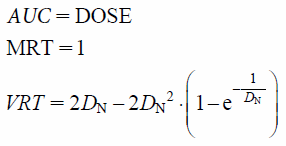 | (6) |
Data on 35 points in 0.1 steps from 0.1 to 3.5 were generated by SIMULATION of NONMEM, and the moments were calculated using Napp.14) In addition, infinite extrapolation was performed during moment calculation (DOSE = 20, DN = 0.01, 0.05, 0.2, 1).
Results
Implementation of PREDFILTPREDFILT includes a lower-level subroutine “pred,” which is called directly from the main body of NONMEM, and a lower-level module “filt” to assist with the calculation of “pred.” Furthermore, “filt” includes two subroutines, “eval” and “model.” Subroutine “pred” is responsible for exchanging variables with the main body of NONMEM and defining the error structure of the model. We implemented the algorithm of FILT in “eval,” and perform numerical inverse Laplace transform corresponding to a model expression defined as “model.” The subroutine “model” can be flexibly replaced with the appropriate equations by the user. The source code and a detailed description procedure of PREDFILT is included in the supplementary notes. As prespecified roles of “pred” in NONMEM, “pred” must return the calculated values of the model, including their derivatives, through changes in inter- and intra-subject errors. Derivatives of inter-subject errors are numerically calculated by assuming a fixed interval of changes. The default interval is 1.0e-4 and users can modify the values as needed.
Validation of CalculationTo validate the calculation of PREDFILT, we employed conventional compartment models and a dispersion model. The calculated values of the compartment models were entirely consistent with eight significant digits at all the time points, confirming that PREDFILT calculated these models with sufficient accuracy (Fig. 1a). Similarly, the time course of the dispersion model was calculated reasonably (Fig. 1b), under the moments were in good agreement with the theoretical values of the dispersion model (Table S1). It was proved that the calculations were performed with high accuracy. The analysis result of THOPP which was provided with NONMEM as an example of population data was equivalent to ADVAN’s one, and the accuracy was confirmed also in the population analysis (Table 1).
Table 1. Comparison of Analysis by ADVAN and PREDFILT for Population Data (THEOPP)
| Parameters | ADVAN | PREDFILT |
|---|
| THETA | | |
| KA | 2.77 | 2.77 |
| K | 0.0781 | 0.0781 |
| CL | 0.0363 | 0.0363 |
| Inter-individual variability (OMEGA) | | |
| KA | 5.55 | 5.55 |
| K | 2.4e−4 | 2.4e−4 |
| CL | 0.515 | 0.515 |
| Residual variability (SIGMA) | 0.388 | 0.388 |
| OFV | 104.561 | 104.561 |
The results of PREDFILT and ADVAN were identical and indicating that PREDFILT works well in population analysis.
Discussion
NONMEM can successfully process numerical inverse Laplace transform using the subroutine PREDFILT, which was newly implemented in this study. FILT analysis, performed by Yamaoka et al. between 1989–1990, primarily included dispersion models with one and two compartments for local PK analysis of the liver. Yamaoka et al. also applied FILT for analysis of enterohepatic circulation. In analogous terms, PREDFILT contributes to PK analysis under NONMEM environments.
FILT exhibits high calculation accuracy in the general pharmacokinetic models examined in this study (Fig. 1a, Table S1). The FILT method would be considered to be several orders of magnitude higher than the calculation accuracy of the Runge–Kutta method; although it is difficult to specify quantitatively because the accuracy is heavily dependent on the type of model. It was reported that the second-order FILT used in this study realized further improvements in accuracy compared to previous first-order algorithms.13)
Purves reported that the calculation accuracy of FILT is particularly limited in several types of models that use lag time. Purves also proposed a modification of the calculation scheme.15) Purves’ proposal was incorporated in PREDFILT. However, it should be noted that models with lag time afford continuous zero data in the initial part of the time domain, and an application of numerical inverse Laplace transform to continuous zero is inevitably difficult because it means that absolutely no information can be used. For models with lag time, calculations can be performed far more reasonably by later adding lag time to the time domain after the solution has been obtained through numerical inverse Laplace transformation of the corresponding model without lag time.
It is expected that using the inverse Laplace transform would make modeling more flexible. FILT is theoretically applicable to the analysis of any tree-like response network models comprising complicated combinations of the responses if each step of the response is described by a Laplace transform (i.e., a transfer function). As a transfer function, the well-stirred model, tube model, and dispersion model are applicable. It is also possible to simulate multiple dosing easily by using a transfer function that expresses repetition. Therefore, the connection of responses in series and parallel is denoted by the multiplication and addition of transfer functions, respectively (Fig. 1c). Furthermore, circulation is donated by, sum of an infinite series of transfer functions (Fig. 1c). This means that we can include the tube model and dispersion model as needed in various physiologically based pharmacokinetics and PK–PD models in addition to the well-stirred model. The dispersion model is a model often contrasted with the well-stirred model, explaining the dynamics of a drug in the local organ more naturally than the well-stirred model (Fig. 1b). Dispersion models can also be used for PK–PD analysis, where flexible time delays exist until the onset of the effects of the drug need to be considered. In the cases of ODE models, when the time delay or the variance of the appearance of pharmacological effect differ depending on the situation, changes in the response–time curves cannot be explained by only parameter changes in a particular model, but the dispersion model can adapt these situations flexibly.
On the other hand, the application of FILT would possibly be restricted because it is inapplicable to nonlinear pharmacokinetic analysis. Nevertheless, we and several researchers have already reported appropriate calculation methods of nonlinear dispersion models.14,16) Although the availability of computer applications capable of performing analysis using nonlinear dispersion models is currently limited, we hope that various analysis methods using PREDFILT and further new tools will facilitate flexible modeling and future simulation research.
Conflict of Interest
The authors declare no conflict of interest.
Supplementary Materials
The online version of this article contains supplementary materials.
References
- 1) Piessens R., Huysmans R., Acm Transactions Math Softw Toms., 10, 348–353 (1984).
- 2) Brzeziński D., Appl. Math. Nonlinear Sci., 3, 487–502 (2018).
- 3) Hosono T., Radio Sci., 16, 1015–1019 (1981).
- 4) Yano Y., Yamaoka K., Tanaka H., Chem. Pharm. Bull., 37, 1035–1038 (1989).
- 5) Yano Y., Yamaoka K., Yasui H., Nakagawa T., J. Pharmacokinet. Biopharm., 19, 71–85 (1991).
- 6) Yamaoka K., Kanba M., Toyoda Y., Yano Y., Nakagawa T., J. Pharmacokinet. Biopharm., 18, 545–559 (1990).
- 7) Yano Y., Yamaoka K., Aoyama Y., Tanaka H., J. Pharmacokinet. Biopharm., 17, 179–202 (1989).
- 8) Mager D., Jusko W., Clin. Pharmacol. Ther., 70, 210–216 (2001).
- 9) Brekkan A., Lopez-Lazaro L., Yngman G., Plan E. L., Acharya C., Hooker A. C., Kankanwadi S., Karlsson M. O., AAPS J., 20, 91 (2018).
- 10) Savic R., Jonker D., Kerbusch T., Karlsson M., J. Pharmacokinet. Pharmacodyn., 34, 711–726 (2007).
- 11) Williams P., Ette E., Clin. Pharmacokinet., 39, 385–395 (2000).
- 12) Ette E., Williams P., Ann. Pharmacother., 38, 1907–1915 (2004).
- 13) Hosono T., Electron. Commun. Jpn. Part II Electron., 81, 10–17 (1998).
- 14) Hisaka A., Sugiyama Y., J. Pharmacokinet. Biopharm., 26, 495–519 (1998).
- 15) Purves, J. Pharm. Sci., 84, 71–74 (1995).
- 16) Aiba T., Kubota S., Koizumi T., Biol. Pharm. Bull., 22, 633–641 (1999).

