Prediction of Anti-proliferation Effect of [1,2,3]Triazolo[4,5-d]pyrimidine Derivatives by Random Forest and Mix-Kernel Function SVM with PSO

Abstract

In order to predict the anti-gastric cancer effect of [1,2,3]triazolo[4,5-d]pyrimidine derivatives (1,2,3-TPD), quantitative structure–activity relationship (QSAR) studies were performed. Based on five descriptors selected from descriptors pool, four QSAR models were established by heuristic method (HM), random forest (RF), support vector machine with radial basis kernel function (RBF-SVM), and mix-kernel function support vector machine (MIX-SVM) including radial basis kernel and polynomial kernel function. Furthermore, the model built by RF explained the importance of the descriptors selected by HM. Compared with RBF-SVM, the MIX-SVM enhanced the generalization and learning ability of the constructed model simultaneously and the multi parameters optimization problem in this method was also solved by particle swarm optimization (PSO) algorithm with very low complexity and fast convergence. Besides, leave-one-out cross validation (LOO-CV) was adopted to test the robustness of the models and Q² was used to describe the results. And the MIX-SVM model showed the best prediction ability and strongest model robustness: R² = 0.927, Q² = 0.916, mean square error (MSE) = 0.027 for the training set and R² = 0.946, Q² = 0.913, MSE = 0.023 for the test set. This study reveals five key descriptors of 1,2,3-TPD and will provide help to screen out efficient and novel drugs in the future.

Introduction

Gastric cancer, having become the fifth factor affecting human health and the third common cancer, occurs mainly in South America, East Asia and Eastern Europe, and more than 900000 new cases are reported every year.^1,2) In addition, it is frequently diagnosed in the terminal stage with the survival rate of no more than 20%.^3–5) In recent years, many treatment measures have been attempted to cure gastric cancer, such as chemotherapy, surgical resection, and radiation protocols.⁶⁾ However, none of the solutions achieves perfect results, and gastric cancer may recur even after above treatment methods.⁶⁾ Therefore, developing some safer and more effective drugs has become a major focus on gastric cancer research.

In the past studies, it has been proved that heterocycles play a major role in the discovery and development of new drugs.⁷⁾ [1,2,3]Triazolo[4,5-d]pyrimidine derivatives (1,2,3-TPD) are typical heterocyclic molecules, which are composed of two active compounds, triazole and pyrimidine.^8,9) Furthermore, 1,2,3-TPD have been extensively studied and proved to have good antitumor effects.⁷⁾ In previous literature,^9–12) in order to study their effect on gastric cancer, 1,2,3-TPD were screened in vitro anti-proliferation against a gastric cancer cell line, MGC-803 (human gastric cancer cells) using the 3-(4,5-dimethylthiazol-2-yl)-2,5-diphenyltetrazolium bromide (MTT) assay method, and 5-fluorouracil (5-Fu) was used as a positive control.¹²⁾ More importantly, IC₅₀ values on MGC-803 have been measured with too much manpower and material resources.¹²⁾

The models of quantitative structure–activity relationship (QSAR) can not only save a lot of human and financial resources but also predict the properties of new compounds quickly and precisely.¹³⁾ QSAR models can be established based on several precisely selected molecular descriptors, which are responsible for the corresponding activity of compounds and the subsequent data analysis.^14,15)

In this study, QSAR models were established by the heuristic method (HM), random forest (RF), support vector machine with radial basis kernel function (RBF-SVM), and mix-kernel function support vector machine (MIX-SVM) including radial basis kernel and polynomial kernel. In addition, because MIX-SVM introduced more parameters, the particle swarm optimization (PSO) algorithm was adopted in the process of constructing model to improve the speed and accuracy of optimizing parameters. In addition, the model constructed by RF shows great performance, which not only explains the importance of the selected descriptors but verifies the validity of employing the same descriptors to other models. Furthermore, the model constructed by MIX-SVM fits the data best and exhibits the strongest robustness. In general, this study may provide salient help in studying the descriptors or substituents to improve the activity in the 1,2,3-TPD fields.

Experimental

Data Preparation

All compounds (1–70) and their MGC-803 IC₅₀ values studied in this paper were from literatures.^9–12) Moreover, the inhibitory activity was measured by Geng et al. after 72 h of exposure to the substance and expressed as the concentration, and IC₅₀ values of each compound were measured and averaged for three times, which guaranteed high accuracy and small error.¹¹⁾ The compounds and their IC₅₀ values used in this study are given in Table 1 and all compounds were randomly divided into the training set and test set in the proportion of 4 : 1. The training set containing 56 compounds was used to build the models, whereas the remaining 14 compounds constituted the test set, and were used to evaluate the performance of the models.

Table 1. Measured and Predicted −lg (IC₅₀) of 1,2,3-TPD

*Test set.

Calculation of the Descriptors

The calculation of molecular descriptors is the basis of QSAR research, which determines the precision and accuracy of the models. At present, the descriptors are commonly calculated by some software such as Cerius2, Sybyl, Dragon, and CODESSA.¹⁶⁾ In this study, CODESSA was used to calculate the descriptors, HM was used to select several key descriptors, and RF was adopted to verify the validity of the selected descriptors.

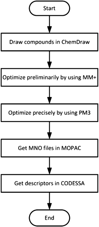
The process of obtaining descriptors consists of two stages. The first stage includes drawing and optimization under the guidance of the theory that the lower the energy of a molecule is, the more stable its structure is. In order to obtain the most stable structure, a series of optimizations were carried out for the molecular as the flow chart shown in Fig. 1. All compounds were drawn by ChemDraw and optimized in HyperChem software.¹⁷⁾ In the optimization process, pre-optimized was performed using the MM+ molecular mechanic’s force field and a semi-empirical PM3 method was subsequently adopted to obtain the molecule with the lowest energy. The second stage is to generate five categories of descriptors: The files of optimized molecule structure from the first stage were imported in MOPAC¹⁸⁾ to obtain MNO files which were the input of CODESSA.¹⁹⁾ Then the calculation was performed in CODESSA to get five classes of descriptors: constitutional, topological, geometrical, electrostatic, and quantum chemical.²⁰⁾ In general, the aim of these two stages is finding accurate descriptors, which is a critical premise for building QSAR models in the next step.

Fig. 1. The Steps of Calculation Descriptors

Linear Model by HM^21,22)

HM is a common and effective method for selecting descriptors, which has been proved in some previous literatures.^23–27) Therefore, HM was adopted to determine the concrete descriptors calculated from CODESSA in previous step. This method is not only effective but also has no limitation on the size of the dataset. A pre-selection of descriptors should be carried out before establishing models by HM: First, some non-universal descriptors are discarded for all structures and those with constant values are also rejected. In addition, if the correlation coefficient of the selected descriptors is greater than 0.8, these descriptors are collinear descriptors and should be discarded. Thus, the total number of descriptors will decrease greatly and linear models can be built.

In this study, R² and mean square error (MSE) were used to test the models established by HM, RF, RBF-SVM, and MIX-SVM. In addition, leave-one-out cross-validation (LOO-CV) was adopted to verify the robustness of all models and the cross validation correlation coefficient (Q²) was used to describe the results.

Nonlinear Model by RF

Since the IC₅₀ value of 1,2,3-TPD is affected by various and complex factors, linear models can not predict the IC₅₀ of 1,2,3-TPD accurately. Therefore, three nonlinear QSAR models were established by RF, RBF-SVM, and MIX-SVM. RF is a novel and effective tool for QSAR modeling, which can predict biological activities of compounds and evaluate the importance of the descriptors by GINI coefficients.^28,29)

In general, RF will be divided into two parts. The first part is to perform feature selection from all descriptors from CODESSA. Within a random forest, each tree provides the most important descriptors from this subset.³⁰⁾ And then the predictions of all the trees will be averaged and the most relevant descriptors will be generated.³⁰⁾ These descriptors will be sorted according to Gini coefficients in descending order and those with higher Gini coefficients are more important. The second part is building RF regression models. In RF algorithm, three parameters need to be determined: the number of trees n, the max depth of trees d, and the number of the relevant features f.³¹⁾

In this study, two RF models was constructed firstly with hundreds of descriptors from CODESSA and several descriptors determined by HM, respectively. The former was to perform descriptors selection to substantiate the efficacy of descriptors selected from HM, and the latter was used to compare with models built by other nonlinear methods. If the prediction performance is comparable or better than other models, the resulting Gini coefficients can be used to explain the importance of the descriptors. Furthermore, different number of descriptors were selected and used to construct RF models according to Gini coefficients. If the descriptors obtained by RF have many overlaps with those selected by HM and their performance is comparable, the validity of the descriptors will get demonstrated.

Nonlinear Model by RBF-SVM

SVM is an efficient supervised machine learning algorithm, which was proposed by Vapnik and his colleagues in 1964.³²⁾ Over the past few decades, SVM has been widely used and achieved remarkable results in solving classification and regression problems in various fields.^33–36) SVM is also termed support vector regression (SVR) when it is applied to regression.

The main idea of the SVR algorithm is as follows: Mapping data points from an input space of dimension X to a feature space of higher dimension F by a non-linear transformation U(x), and then performing linear regression in F space.^37,38) In order to realize the inner product logical relationship and reduce the computational complexity in high-dimensional space, the kernel function is adopted. Furthermore, some parameters like ε-insensitive loss function, punish coefficient C, and slack variables ξ_i, ξ*_i are introduced in SVR. The final constrained optimization problem becomes the following formula Eq. (1):

  

(1)

In Eq. (1), the first term (y_i − w·x_i − b ≤ ε + ξ_i) is adopted to make the regression function smoother and enhance generalization performance, while the second term (w･x_i + b−y_i ≤ ε + ξ_i*) is defined to reduce errors.

Then, the minimum value can be obtained by building the Lagrange equation and calculating partial differential coefficients. Finally, the regression function of SVR is as follows in Eq. (2):

  

(2)

where κ(x_i, x) = <U(x_i), U(x) > is the kernel function including radial basis kernel, polynomial kernel, sigmoid kernel, and so on; n represents the number of support vectors; α_i* and α_i are Lagrange multipliers; and b can be calculated when the conditions in Eq. (1) becomes equal. In this method, the radial basis kernel is Eq. (3):

  

(3)

where γ can be regarded as the reciprocal of the scope of the supported vector. Larger γ will lead to over fitting and lower generalization while smaller γ will result in under fitting.

Nonlinear Model by MIX-SVM

Compared with RBF-SVM, the MIX-SVM method introduces polynomial kernel function on the basis of retaining radial basis kernel function. As a local function, radial basis kernel function has strong learning ability but weak generalization ability, while polynomial kernel function is just the opposite.^39–41) Therefore, a mix-kernel function combining polynomial and radial basis kernel function is constructed, which has the advantages of strong learning and generalization abilities simultaneously.

The polynomial kernel function follows Eq. (4):

  

(4)

where d is the degree of the polynomial kernel function.

From Eq. (3) and Eq. (4), the mix-kernel function form is as in Eq. (5):

  

(5)

where d, γ, and ω are the degree of the polynomial kernel function, the radial basis kernel parameter, and the mixing weight coefficient respectively. ω∈[0, 1], and if ω = 1, the mix-kernel function is the radial basis kernel; if ω = 0, the mix-kernel function is the polynomial kernel function.

The Theory of PSO

In the MIX-SVM method, multiple parameters need to be determined, including the radial basis kernel function parameter γ, penalty coefficient C, polynomial kernel function parameter d, and mixing weight ω. Therefore, the computation will be very complicated if the grid search method is adopted. In order to improve the speed and accuracy of optimizing parameters, the PSO algorithm proposed by Kennedy and Eberhart in 1995 was used in this work.⁴²⁾

The PSO is based on the study of the predation behavior of flocks. In PSO, each particle is a n-dimensional point, and different particles have individual fitness.^43–45) In each iteration, the particle updates itself by tracking the individual extreme value p_best and the global extreme value g_best.^46,47) During the tracking process, the particles update their speed and position through the following two Eqs:

  

(6)

  

(7)

The process of optimizing SVM parameters by PSO is as follows:

1. (1)    Randomly generate initial positions and velocities of a set of particles.
2. (2)    Determine the value range of the parameters being optimized.
3. (3)    Calculate the fitness of each particle.
4. (4)    Update the individual extreme value p_best and the global extreme value g_best according to the fitness value.
5. (5)    Update the velocity and location of the particle according to Eq. (6) and Eq. (7). Check the end condition.
6. (6)    Obtain the best parameters set.

Results and Discussion

Results of HM

Four hundred thirty four descriptors were calculated by CODESSA. In order to obtain several descriptors which were most relevant to 1,2,3-TPD, the number of molecular descriptors in linear models was increased from 1 to 7 and the corresponding R² and R²_cv were recorded. When one more molecular descriptor was added and R² and R²_cv no longer increased intensely, the number of descriptors was determined. The influence of the number of descriptors on R² and R²_cv is shown in Fig. 2.

Fig. 2. Influence of the Number of Descriptors on R² and R²_cv

As shown in Fig. 2, R² of linear models increases slightly when the number of descriptors changes from 5 to 6. Therefore, five descriptors are selected and their symbols and physical-chemical meaning are shown in Table 2. At the same time, their correlation coefficients are shown in Table 3, which are much smaller than 0.8.

Table 2. The Descriptors Selected by HM and Their Physical-Chemical Meaning

Symbol	Physical-chemical meaning
MEAHN	Max e–n attraction for a H–N bond
MVC	Max valency of a C atom
MBON	Min (>0.1) bond order of a N atom
MERIC	Max electroph react index for a C atom
M1RIS	Min 1-electron react index for a S atom

Table 3. Correlation Matrix of the Five Descriptors

Descriptor	MEAHN	MVC	MBON	MERIC	M1RIS
MEAHN	1	−0.12	0.26	0.51	−0.05
MVC		1	−0.07	−0.12	−0.003
MBON			1	−0.04	0.09
MERIC				1	−0.04
M1RIS					1

R² and MSE of the training set and test set in the model were 0.775, 0.774, and 0.083, 0.092, respectively, and the plot of HM is shown in Fig. 3. Furthermore, Q² of LOO-CV of the training set and test set in HM were 0.775 and 0.776.

Fig. 3. The Plot of Measured and Predicted −lg (IC₅₀) by HM

The mathematical expression of the HM model followed Eq. (8):

  

(8)

where d₁, d₂, d₃, d₄, and d₅ represented MEAHN, MVC, MBON, MERIC, and M1RIS, respectively.

Results of RF

After optimizing the parameters using grid search, the optimal parameters n, and f were 10 and 5, respectively. The value of d was set to the default in python libraries. When using the 434 descriptors, R² of training set and test set were 0.907 and 0.65, and MSE of training set and test set were 0.035 and 0.148, respectively. Meanwhile, the descriptors were calculated according to the Gini coefficient. As shown in Fig. 4, there are three same descriptors (MEAHN, MERIV, and MVC) among the descriptors selected by RF and HM respectively, which reveals the importance of the three descriptors and the validity of the HM to a certain extent. In addition, Fig. 5 shows the optimal prediction results of RF regression with five descriptors determined by HM. R² of the training set and test set were 0.92 and 0.833, and their MSE were 0.03 and 0.07. When LOO-CV was executed, Q² of the training set and test set were 0.936 and 0.861. Table 4 showed the RF prediction performance with different number (3, 5, and 7) descriptors with high Gini coefficient. The results showed that their predictions are slightly weaker than the model with descriptors by HM. Therefore, the descriptors (MEAHN, MVC, MBON, MERIC, and M1RIS) selected by HM were important and HM was proved to be a reasonable tool for selecting descriptors.

Fig. 4. The Descriptors Selected by RF

Fig. 5. The Plot of Measured and Predicted –lg (IC₅₀) by RF

Table 4. The RF Models with Different Number of Descriptors Selected by RF

Number of descriptors	R2		MSE		Q2
	Training set	Test set	Training set	Test set	Training set	Test set
3 Descriptors	0.928	0.782	0.027	0.092	0.926	0.828
5 Descriptors	0.930	0.79	0.026	0.089	0.923	0.84
7 Descriptors	0.931	0.747	0.026	0.107	0.928	0.843

Results of RBF-SVM

Since the validity of the descriptors has been proved, the five descriptors determined by HM could be adopted when building other nonlinear models. The SVM method using the radial basis function should determine several parameters: punishment parameter C, ε-insensitive loss function, and corresponding parameters of the radial basis kernel function. As a regularization parameter, too large C will lead to over fitting of the model, while too small C is easy to fall into under fitting. The ε-insensitivity stops the entire training set satisfying boundary conditions, which provides the possibility of a sparse solution.

The form of the radial basis function is as Eq. (3), where γ is a constant. Smaller γ means more support vectors, which affects the training speed of the model greatly. Using the grid search method, the optimal values of C, γ, and ε were 189.64, 4.43, and 0.1 respectively. The optimal prediction results of RBF-SVM are given in Fig. 6. R² of the training set and test set were 0.919 and 0.902, and their MSE were 0.03 and 0.042. When LOO-CV was executed, Q² of the training set and test set were 0.912 and 0.882.

Fig. 6. The Plot of Measured and Predicted −lg (IC₅₀) by RBF-SVM

Results of MIX-SVM

The MIX-SVM has more parameters than the RBF-SVM, so the PSO algorithm was used to optimize parameters. The PSO algorithm avoided trying all parameter combinations and converged fast, which could be used for searching the optimal solution with low computational complexity. The particle swarm size and iteration number were set to 50 and 100 respectively. According to the results of previous works, the inertia factor λ the learning factors c₁ and c₂ which are listed in Eq. (6) were set as 0.5, 2, 2.

After optimizing parameters via PSO, the optimum C = 169.9, γ = 5.63, ω = 0.95, and d = 2 were obtained, which meant that the radial basis function had a weight of 0.95, and the weight of polynomial kernel function was only 0.05. The optimization results in each iterator are shown in Fig. 7. In addition, it can be found that the fitness value has fluctuated slightly after the twentieth generation. Figure 8 gives the most optimal prediction results of MIX-SVM. R² of the training set and test set were 0.927 and 0.946, and their MSE were 0.027 and 0.023. When LOO-CV was executed, Q² of the training set and test set were 0.916 and 0.913. The robustness of the model using two kernel functions was better than that just using radial basis kernel function.

Fig. 7. The Fitness of Each Generation

Fig. 8. The Plot of Measured and Predicted −lg (IC₅₀) by MIX-SVM

Discussion

The results of the four models are shown in Table 5. Compared with HM, RF achieves excellent performance and shows strong robustness. Among the descriptors selected by RF and HM respectively, there are three same descriptors (MEAHN, MERIV, and MVC). This indicates the accuracy of employing the same five descriptors of HM to other models. Due to the low computation cost and great prediction performance, RF will play a key role in the research field of machine learning for inhibitory activity of compounds. In addition, since the advantages and disadvantages of the polynomial kernel function and the radial basis kernel function complement each other, MIX-SVM fits the data better and does not overfit. Furthermore, Q² of LOO-CV of the training set and test set are shown in Table 6, which shows that RF, RBF-SVM and MIX-SVM models are more robust than HM.

Table 5. Comparison of Prediction Results of Different Methods

Method	R2		MSE
	Training set	Test set	Training set	Test set
HM	0.775	0.774	0.083	0.092
RF	0.92	0.833	0.03	0.07
RBF-SVM	0.919	0.902	0.03	0.042
MIX-SVM	0.927	0.946	0.027	0.023

Table 6. Comparison of LOO-CV Results of Different Methods

Method	Q2 (Training set)	Q2 (Test set)
HM	0.775	0.776
RF	0.936	0.861
RBF-SVM	0.912	0.882
MIX-SVM	0.916	0.913

Among the five descriptors, MEAHN is the most important one because it is always selected as the top node and has the highest Gini coefficient in the models built by RF. As a quantum chemical descriptor, MEAHN reflects the attraction drive processes between the electron and nucleus, which is likely related to conformational changes or atomic reactivity in the molecule. The second descriptor MVC is a quantum chemical descriptor, which ranges over the strength of intramolecular bonging and illustrates the stability of the molecules and their conformational flexibility. Trying to decrease the valency of C atom in substituents may contribute to decrease the value of IC₅₀ on MGC-803. The descriptor, MBON, is also a quantum chemical descriptor, which indicates the strength of covalent bond in the molecule. MERIC, as an electrostatic descriptor, shows the properties of different charge distribution. Related to the distribution of the charge in the molecular structure, M1RIS estimates the relative reaction ability of the C atoms and is related to the activation energy of the reaction. Furthermore, the coefficients of the four descriptors (MEAHN, MVC, MBON, and MERIC) are negative, which indicates IC₅₀ on MGC-803 will decrease as the values of the four descriptors decrease. And M1RIS is the opposite, the higher its value is, the more IC₅₀ drops.

Since the compounds with numbers 14 and 17 in Table 1 have lower IC₅₀, the similar other molecules with above descriptors may be a novel anti-gastric cancer inhibitor and can be designed a potential drug. In general, this study reveals the correlation between anti-gastric cancer effect and the five important descriptors, which will provide a research focus on the design of novel 1,2,3-TDP in future.

Conclusion

The models built by RF and MIX-SVM show great prediction performance and strong robustness. It is believed that the models constructed by RF and MIX-SVM may have a wide application prospect in the research of 1,2,3-TPD. Furthermore, this study also reveals five key descriptors that influence the anticancer effect of 1,2,3-TPD: Max e-n attraction for a H–N bond, Max valency of a C atom, Min (>0.1) bond order of a N atom, Max electroph react index for a C atom, and Min 1-electron react index for a S atom, which will provide some guidance on these descriptors for the development of potential new drugs on 1,2,3-TPD in the future.

Acknowledgments

The authors are very grateful to these software: PyCharm Community Edition 2021.1.1 × 64 JetBrains, ChemDraw Ultra 8.0 CambridgeSoft, HyperChem Professional, and CODESSA Katritzky, A. R. And we are grateful to anonymous learned referees whose valuable comments improve the quality of the paper.

Conflict of Interest

The authors declare no conflict of interest.

References

• 1) Arnold M., Karim-Kos H. E., Coebergh J. W., Byrnes G., Antilla A., Ferlay J., Renehan A. G., Forman D., Soerjomataram I., Eur. J. Cancer, 51, 1164–1187 (2015).
• 2) Goetze O. T., Al-Batran S. E., Chevallay M., Mönig S. P., Monig S. P. UPDATES IN SURGERY, 70, 173–179 (2018).
• 3) Siegel R. L., Miller K. D., Jemal A., CA Cancer J. Clin., 70, 7–30 (2020).
• 4) Siegel R. L., Miller K. D., Jemal A., CA Cancer J. Clin., 69, 7–34 (2019).
• 5) Ajani J. A., D’Amico T. A., Almhanna K., et al., J. Natl. Compr. Canc. Netw., 14, 1286–1312 (2016).
• 6) Coccolini F., Cotte E., Glehen O., Lotti M., Poiasina E., Catena F., Yonemura Y., Ansaloni L., Eur. J. Surg. Oncol., 40, 12–26 (2014).
• 7) Pitucha M., Wos M., Miazga-Karska M., Klimek K., Miroslaw B., Pachuta-Stec A., Gladysz A., Ginalska G., Med. Chem. Res., 25, 1666–1677 (2016).
• 8) Megally Abdo N. Y., Kamel M. M., Chem. Pharm. Bull., 63, 369–376 (2015).
• 9) Geng P. F., Liu X. Q., Zhao T. Q., Wang C. C., Li Z. H., Zhang J., Wei H. M., Hu B., Ma L. Y., Liu H. M., Eur. J. Med. Chem., 146, 147–156 (2018).
• 10) Xu C. H., Zhou W. J., Dong G. J., Qiao H., Peng J. D., Jia P. F., Li Y. H., Liu H. M., Sun K., Zhao W., Bioorg. Chem., 105, 104424 (2020).
• 11) Li Z. H., Yang D. X., Geng P. F., Zhang J., Wei H. M., Hu B., Guo Q., Zhang X. H., Guo W. G., Zhao B., Yu B., Ma L. Y., Liu H. M., Eur. J. Med. Chem., 124, 967–980 (2016).
• 12) Li Z. H., Liu X. Q., Zhao T. Q., Geng P. F., Guo W. G., Yu B., Liu H. M., Eur. J. Med. Chem., 139, 741–749 (2017).
• 13) Wang Y., Liu Z., Qu A. L., Zhang P. J., Si H. Z., Zhai H. L., Latin American Journal of Pharmacy, 39, 1159–1170 (2020).
• 14) Davis G. D. J., Vasanthi A. H. R., Eur. J. Pharm. Sci., 76, 110–118 (2015).
• 15) Vasanthanathan P., Lakshmi M., Arockia Babu M., Gupta A. K., Kaskhedikar S. G., Chem. Pharm. Bull., 54, 583–587 (2006).
• 16) Ren W., Kong D., Computers and Applied Chemistry, 26, 1455–1458 (2009).
• 17) Inc. H., Hyperchem Version 4.0. Hypercube Inc., Ontario, 1994.
• 18) Stewart J. J. U. I., MOPAC 6.9, Bloomington In., U.S.A., 1989.
• 19) Katritzky A. R., Perumal S., Petrukhin R., Kleinpeter E., J. Chem. Inf. Comput. Sci., 41, 569–574 (2001).
• 20) Wright J. S., Carpenter D. J., McKay D. J., Ingold K., J. Am. Chem. Soc., 119, 4245–4252 (1997).
• 21) Katritzky A. R., Mu L., Lobanov V. S., Karelson M., J. Phys. Chem., 100, 10400–10407 (1996).
• 22) Tong W., Lowis D. R., Perkins R., Chen Y., Welsh W. J., Goddette D. W., Heritage T. W., Sheehan D. M., J. Chem. Inf. Comput. Sci., 38, 669–677 (1998).
• 23) He D., Ma J., Shi X., Zhao C., Hou M., Guo Q., Ma S., Li X., Zhao P., Liu W., Yang Z., Mou J., Song P., Zhang Y., Li J., Chem. Pharm. Bull., 62, 967–978 (2014).
• 24) Yang B., Si H. Z., Zhai H. L., Lett. Drug Des. Discov., 18, 406–415 (2021).
• 25) Li Y. Q., You G. R., Jia B. X., Si H. Z., Yao X. J., Biomed Research International, 2014, 216072 (2014).
• 26) Wang W. X., Si H. Z., Zhang Z. D., Mol. Simul., 38, 38–44 (2012).
• 27) Si Y. R., Xu X. Y., Hu Y. F., Si H. Z., Zhai H. L., Chem. Biol. Drug Des., 97, 978–983 (2021).
• 28) Svetnik V., Liaw A., Tong C., Culberson J. C., Sheridan R. P., Feuston B. P., J. Chem. Inf. Comput. Sci., 43, 1947–1958 (2003).
• 29) Polishchuk P. G., Muratov E. N., Artemenko A. G., Kolumbin O. G., Muratov N. N., Kuz’min V. E., J. Chem. Inf. Model., 49, 2481–2488 (2009).
• 30) Inthajak K., Khamsemanan N., Nattee C., Toochinda P., Lawtrakul L., Monatsh. Chem., 148, 1697–1709 (2017).
• 31) Tyralis H., Papacharalampous G., Langousis A., Water, 11, 910 (2019).
• 32) Burges C. J. C., Data Min. Knowl. Discov., 2, 121–167 (1998).
• 33) Cai C. Z., Wang W. L., Sun L. Z., Chen Y. Z., Math. Biosci., 185, 111–122 (2003).
• 34) Cai C. Z., Han L. Y., Ji Z. L., Chen X., Chen Y. Z., Nucleic Acids Res., 31, 3692–3697 (2003).
• 35) Cai C. Z., Wang W. L., Chen Y. Z., Int. J. Mod. Phys. C, 14, 575–585 (2003).
• 36) Song J. N., Burrage K., BMC Bioinformatics, 7, 425 (2006).
• 37) Khemchandani R., Jayadeva, Chandra S., Expert Syst. Appl., 36, 132–138 (2009).
• 38) Collobert R., Bengio S., J. Mach. Learn. Res., 1, 143–160 (2001).
• 39) Zheng S., Liu R., Tian J. W., ieee, An SVM-based small target segmentation anuclustering approach. “Proceedings of the 2004 International Conference on Machine Learning and Cybernetics,” Vols. 1–7, 2004, pp. 3318–3323.
• 40) Zheng Z., Xu W., Xu F., Liu Z., Rock and Soil Mechanics, 33, 1421–1426 (2012).
• 41) Zhong Z., Carr T. R., Fuel, 184, 590–603 (2016).
• 42) Eberhart R. C., Shi Y., IEEE Trans. Evol. Comput., 8, 201–203 (2004).
• 43) Li A., Qin Z., Bao F., He S., Computer Engineering and Application, 38, 1–3 (2002).
• 44) Yang W., Li Q., Eng. Sci., 6, 87–94 (2004).
• 45) Sheng-wei F. E. I., Yu-bin M., Cheng-liang L. I. U., Xiao-bin Z., High Voltage Engineering, 35, 509–513 (2009).
• 46) Lin S. W., Ying K. C., Chen S. C., Lee Z. J., Expert Syst. Appl., 35, 1817–1824 (2008).
• 47) Subasi A., Comput. Biol. Med., 43, 576–586 (2013).