Original papers
Analysis of the Color Developed during Carbonization of Grilled Fish by Kinetics and Computer Imaging
2014 Volume 20 Issue 5 Pages 1051-1061
Details
2014 Volume 20 Issue 5 Pages 1051-1061
Samples of red sea bream (Pagrus major) were grilled under far-infrared radiation heating. The last step of grilling, namely, carbonization, was analyzed. The temperature and color CIE L*a*b* at the center of the fish surface were measured during the entire grilling process. The color that developed during the carbonization was analyzed using a kinetic model based on the reduction rate of L* values and a computer vision system (CVS). Empirical equations for estimating a* and b* values were deduced based on the calculated L* values. During the carbonization step, the L* values of the surfaces decreased slowly. The L* values appeared to reach a constant value, the magnitude of which depends on the surface temperature. The color distribution across the entire surface during the grilling process was effectively estimated using the CVS. The effect of surface temperature on carbonization was analyzed by the CVS and successfully visualized using a two-dimensional simulation model.
The surface color of food is one of the important characteristics of baked, grilled, and broiled products and may be a critical index for consumer acceptance (Onishi et al., 2011). The process of grilling comprises four steps: (1) protein denaturation, (2) water evaporation, (3) a browning reaction, and (4) a carbonization reaction (Nakamura et al., 2011), and there is a change in the surface color of food associated with almost each step. Browning, a Maillard-type reaction, occurs at low levels of available water; therefore, it is common in dry cooking methods, such as grilling, in which the surface layer is dehydrated. Sustained heating of dry surfaces eventually results in carbonization, i.e., thermal conversion of organic materials to carbon (Lewis, 1982), and is usually accompanied by the generation of smoke. During heating, the surface of food first turns brown, following which the surface blackens as it burns (Rosenthal, 2003). One of the most obvious disadvantages associated with the carbonization of food is the loss in the nutritive value of the proteins in the food; moreover, the increase in cooking temperature and time negatively affects the food's appearance (Broyart et al., 1998; Hosseinpour et al., 2013). The cooking temperature and time play a particularly important role during the grilling process, because at the end of the process, the surface temperature is mostly over 150°C (Llave et al., 2014b; Matsuda et al., 2013; Wang et al., 2011). Excessive heating promotes a series of chemical reactions in protein-rich foods such as fish; thus, the entire grilling process should be controlled by selecting the optimal final grilling temperature based on the color and appearance of the grilled surface. Therefore, to increase both food quality and safety, it is important to analyze color formation during the last step of the grilling process (carbonization) in detail by experimental and mathematical modeling approaches.
A computer vision system (CVS) has been reported to be suitable for acquiring and analyzing the image of a real scene by computers for obtaining the information or controlling the processes (Brosnan and Sun, 2004). Moreover, it has been documented more advantageous over the traditional techniques (Brosnan and Sun, 2004; Yam and Papadakis, 2004), since a CVS is non-invasive, fast, inexpensive, and utilizes a precise technique for measuring and modeling the color of foodstuffs during processing (Hosseinpour et al., 2013).
In this study, the effect of surface temperature on color changes during the grilling of fish (beginning of the carbonization step) by using a kinetic model and the use of a CVS as an effective process control in the food industry were evaluated. The browning and darkening were visualized at different time intervals by using a two-dimensional (2D) model for browning, which we developed in our previous study (Llave et al., 2014b).
The browning and carbonization were visualized using a previously developed 2D model (Llave et al., 2014b). The color formation was modeled according to the intensity of the color change and did not directly involve chemical compounds. Thus, the color at the center of the fish surface during grilling was accurately estimated by the combination of the protein denaturation model (Yu et al., 2014), browning kinetic model (Matsuda et al., 2013), and carbonization kinetic model developed in this study.
Assuming that an original substance P (reactant P) is transformed into a charred substance C and smoke substance G of amount “a” on heating (Eq. 1) and that the production rate of C is proportional to the remaining concentration of P, the reaction rate can be expressed by Eq. 2.
 |
Here, G is assumed to be generated in a certain percentage of C.
 |
Here, CP, CC, and CG are the concentrations of P, C, and G, respectively, and k is the rate constant. Assuming that there is no G initially and that all of P changes into C, the initial and final concentrations are expressed as follows:
Initial conditions:
 |
Final conditions:
 |
where subscripts i and f represent the initial and final values, respectively, and C0 is the total concentration of P plus C and G. When CC increases from CCi to CCf, the sample darkens, i.e., L* decreases from L*i to L*f. Assuming that the decrease in L* is proportional to the concentration of C, the dimensionless parameter Y can be expressed as follows:
 |
When Eq. (5) is substituted into Eqs. (2) and (3), the following equation is obtained:
 |
We assumed that the temperature dependence of the rate constant follows the Arrhenius equation as follows:
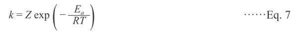 |
where Z is the pre-exponential factor, Ea is the activation energy during the carbonization, and R is the gas constant. The pre-exponential factor and activation energy were evaluated using Eq. (8), which is obtained when Eq. (7) is substituted into Eq. (6):
 |
Thus, when the pre-exponential factor and activation energy are given and the experimental time-temperature information is used, Y can be calculated by the numerical integration of Eq. (8).
Materials Red sea bream (Pagrus major) was used as the sample in this study. This fish species was chosen because it is commonly used for grilling. Red sea bream was purchased from a local fish market on the day of the experiment, and in all the cases, the fish samples were under rigor mortis. The skin and bones were removed, and the ordinary muscle of the fillets was cut into 3 × 4 × 1.5 cm3 samples for all the experiments. The samples were wrapped in a film and refrigerated at 5°C for no more than 30 min before use.
Experimental conditions The dimensions of the far-infrared radiation (FIR) heater (100 V/750 W; electric ceramic plate heater PLC-328, Noritake Co., Aichi, Japan) was 12 × 12 cm2. The infrared energy radiated downward from the heater. The samples were positioned ∼8 cm below the heat source on an electronic balance. The FIR heater was warmed up for 30 min before starting the experiment and adjusted to 400°C. Two experiments were conducted. In the first one, the surface temperature was controlled without using any device. In the second one, after the surface temperature was raised to 160, 180, and 200°C, the temperature was regulated manually by moving the FIR heater with respect to the sample. In this last case, the temperature at the sample point during the different steps was verified to be 160.2 ± 1.2°C, 180.6 ± 0.9°C, and 200.0 ± 1.5°C during the grilling. The radiation energy was measured along with the temperature during the different steps using a radiation sensor (RF30 Captec, Villeneuve d'Ascq, France) at the same sample position. Thus, for example, at a distance of 8 cm between the heater and the sample, the radiation energy was 2.7 × 10⁴ Wm−2. This value decreased with increasing distance.
Surface temperature measurements The surface temperatures of the samples were measured using a K-type thermocouple (ϕ = 0.5 mm) at the center. A single measurement profile was collected for each run using the sample with the longest grilling time. A personal computer, data logger (Thermodac 5001A, Eto Denki Co., Tokyo, Japan), and software (Thermodac-E/Ef 2.6, Eto Denki Co.) were used to collect the temperature data. The accuracy of the surface temperature profiles collected using the K-type thermocouple was verified by comparing them with those collected using IR sensors (Matsuda et al., 2013).
Color measurementsConventional colorimeter The color changes in the fish surface were measured using the CIE L*a*b* system at the same position as the surface temperature measurements, using a spectrophotometric color difference meter (CDM, NF333, Nippon Denshoku Industries Co., Ltd., Tokyo, Japan). The L*a*b* values were measured using a D65 light source with a viewing field angle of 2°. The grilled fish was sampled at 0, 2, 4, 6, 8, 10, 12.5, 15, 17.5, 20, 25, and 30 min. The results are expressed as the mean value of five replications obtained from the center of the surface in each of the five experiments.
Computer vision system A CVS was employed to acquire the entire surface color at each 30 s interval during the grilling.
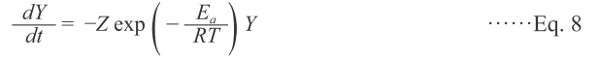
(1) Lighting system: The samples were illuminated using a parallel lamp (with one fluorescent tube, FL20S.D-EDL-D65, natural daylight, 21 W, Toshiba Lighting and Technology, Japan) with a color temperature of 6500 K (D65, a standard light source commonly used in food research) and a color-rendering index (Ra) close to 95%. The lamp (60 cm long) was situated 20 cm above the sample and at an angle of 45° to the sample (Fig. 1).
Diagrammatic representation of the image acquisition system.
(2) Digital camera and image acquisition: A color digital camera (CDC, D5100, Nikon, Japan) was located transversely over the background at a distance of 38 cm in length and 22 cm in height. The angle between the camera lens and axis of the lighting source was 15°. As the standard capture conditions, the following camera settings were tested: a manual mode with the lens aperture, f, of 4.5, 5.0, and 6.0; a shutter speed of 1/125, 1/100, 1/80, and 1/40; a zoom of 32 mm; no flash; an intermediate resolution of the CDC (2464 × 1632) pixels; and the storage were in the JPEG format. The white balance of the camera was set using the same white reference as the CDM.
(3) Image processing: The pre-processing of full images, segmentation from the background, and color analysis were conducted using Adobe Image Ready CS and Adobe Photoshop CS (version 8.0.1). The background was removed from the pre-processed gray-scale image, and the pixel quantity of each territory was determined using the PopImaging software (3.7 Digital being kids Co. Ltd., Yokohama, Japan) to estimate the area of the territory. This segmented image is a binary image, where “0” (black) and “1” (white) indicate the background and object, respectively. Therefore, from this binary image, the localization of the pixels into the interest region allowed us to extract the true color image of the sample from the original image.
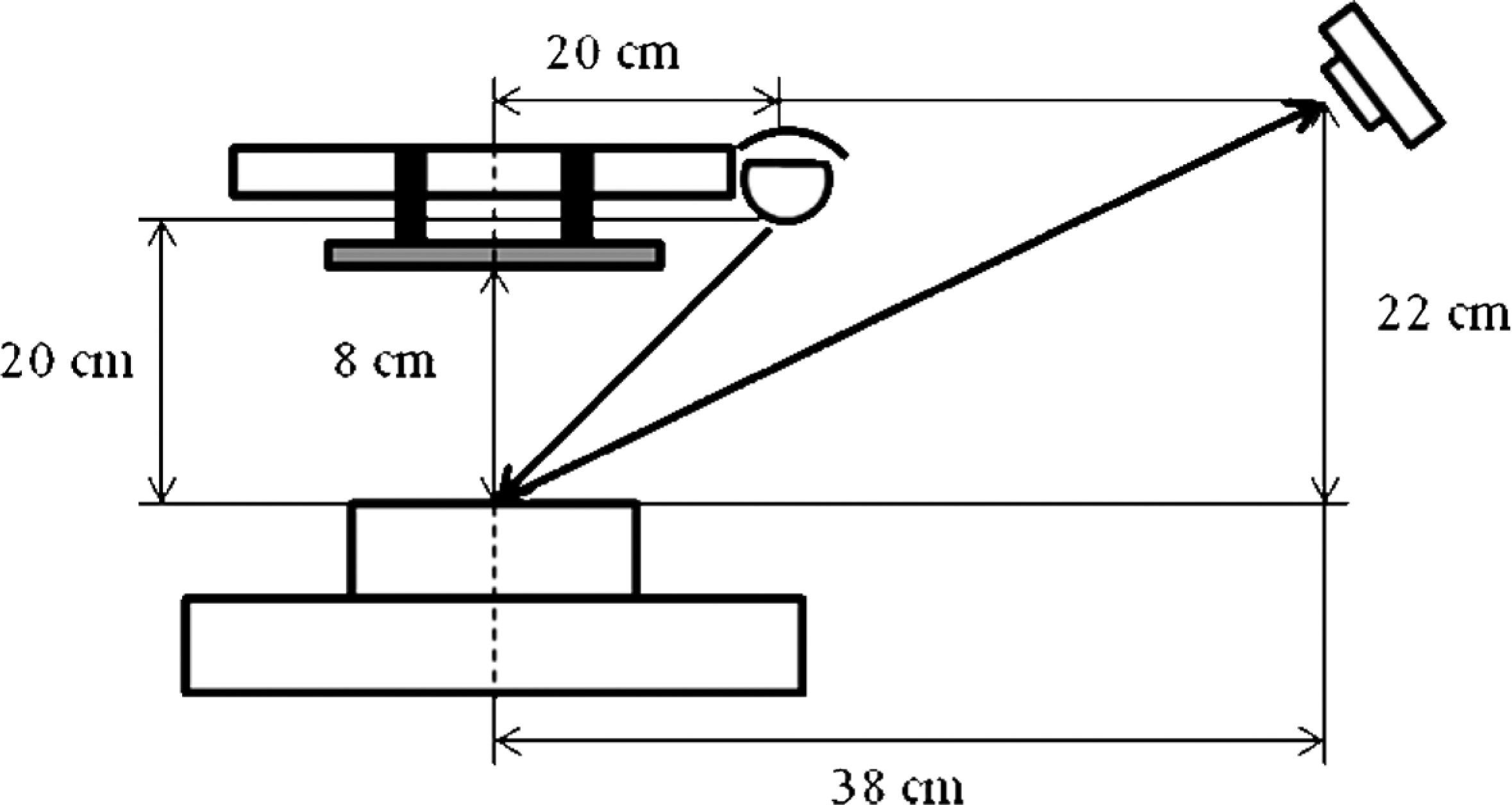
(4) Calibration of the CVS: The color images were characterized using 16 color sheets with different hues (from white to black), corresponding to the possible warm-toned color shown by the grilled fish meat. The colors were photographed and analyzed using the CVS to obtain the R′G′B′ values. Similarly, the L*a*b* values of each color sheet were measured using the CDM at three equidistant points. The comparison of the color results between the CVS and CDM measurements using the same white reference allowed the characterization of the obtained images and confirmation of the suitability of the standard sRGB for the calibration of this particular image acquisition system. The IEC 61966-2-1 (1999) equations that define the transformation from floating point nonlinear R′G′B′ values to CIE XYZ in two steps were used in the same manner as reported by Mendoza et al. (2006) and Larraín et al. (2008).
(i) The nonlinear R′G′B′ values are transformed to linear sRGB values.
When R′G′B′ ≤ 0.04045,
 |
When R′G′B′ > 0.04045,
 |
(ii) Then, using the recommended coefficients by the Rec. ITU-R BT.709-5 (2002), the sRGB values are converted to the CIE XYZ system as follows:
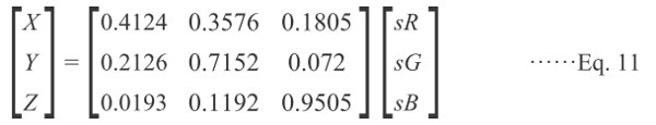 |
In the R′G′B′ encoding process, the power function with a gamma factor of 2.4 includes a slight black-level offset to allow for the invertibility in integer math, which closely fits a straightforward gamma 2.2 curve. Therefore, consistency was maintained using the gamma 2.2 legacy images and the video industry (Mendoza et al., 2006). Also, the sRGB tristimulus values <0.0 or >1.0 were rounded to 0.0 and 1.0, respectively.
Color spaces: In food research, color is often represented using the L*a*b* color space. The definition of L*a*b* is based on the intermediate system, CIE XYZ, which simulates the human perception (Rec. ITU-R BT. 709-5, 2002) and may be converted from the RGB, as shown in Eq. (11). Thus, L*a*b* is defined as follows:
 |
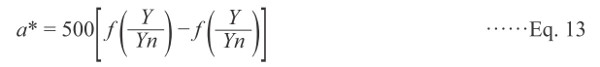 |
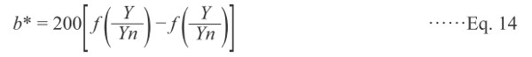 |
where
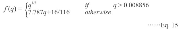 |
Xn, Yn, and Zn are the tristimulus values of the perfect diffuse white surface (95.043, 100.000, 108.879, respectively) for the standard illuminant, D65.
Microscopic inspection of the surface structure After grilling for 30 min, the cross-sections (CSs) of the surface samples were collected and hardened at room temperature (∼25°C). Then, the CSs were embedded and coated on an epoxy resin to provide a protective cover for cutting. The CSs were then mounted on glass slides without polish. The unpolished surfaces of the slabs were kept free of dust prior to the examination under a digital microscope (VHX-1000, Keyence, Japan). A × 100 lens was used and the 2D images were recorded at several positions.
Construction of the 2D model The FEMAP software (10.2, NeiSoftware, CA, USA) was employed to construct the model by selecting the appropriate shape, size, and mesh of the sample (Llave et al., 2014b). Although the three-dimensional (3D) images are shown below, the browning and darkening were evaluated at the upper surface only. Therefore, the analyses of both the processes were simulated in 2D only (X and Y axes). A sample of a 4 × 3 × 1.5 cm3 slab shape was used as the model for all the experiments. The X, Y, and Z coordinates were divided using a mesh spacing of 5 mm, resulting in an 8 × 6 × 3 mesh. The R′G′B′ color data were fed into the model, thus positioning the values at the meshes.
Statistical evaluation The composition data were analyzed by one-way analysis of variance (ANOVA) combined with Tukey's pairwise comparison test using the Systat statistical software (3.5; Systat Software Inc., IL, USA).
Surface color changes of the fish samples Fig. 2 shows the 2D pre-processed images, obtained by the image segmentation technique described above, of the fish surface after 10, 14, 18, 22, 26, and 30 min of FIR heating. The non-uniform color gradually changed from a plain brown to a dark black color. The non-uniform black color may be attributed to the low fat content and heterogeneous temperature distribution of red sea bream during grilling (Llave et al., 2014a). After 8 min of grilling, black spots were observed on the upper surface of the sample as a result of the carbonization because of the highest temperature existing at these positions. The black spots were formed because of dehydration and the effect of the shrinkage phenomenon during grilling.
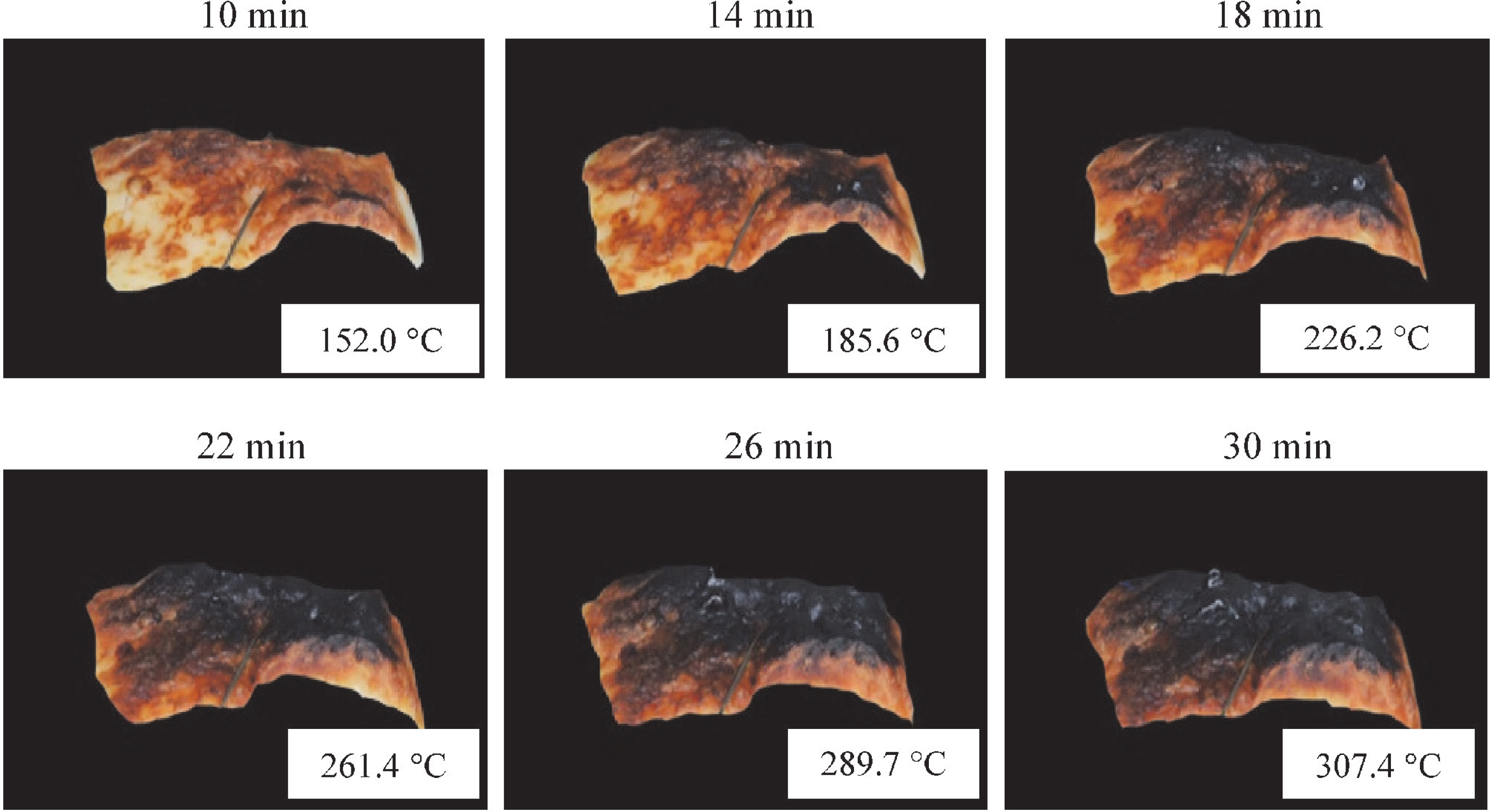
Surface color changes of red sea bream during the last step of FIR grilling.
Analysis of the surface structure of grilled fish at the initial stage of carbonization The structure of the sample surface at the end of the grilling was evaluated by microscopic inspection. For example, the results of the final point of grilling (30 min) are shown in Fig. 3. Three typical structures were observed because of the effect of local chemical reactions on the local temperature. Each of them shows a different final surface temperature (n = 5): 200 – 220°C (A), 170 – 200°C (B), and 150 – 170°C (C). In our previous work (Llave et al., 2014b), a wide temperature distribution of the sample surface at all the time intervals was reported. This heterogeneous temperature distribution was responsible for the non-uniform surface color distribution, particularly for the samples with a low fat content as in the case of the red sea bream used in this study. This explains the different surface structure observed by the microscope, confirming three different steps of the carbonization in the same sample surface.
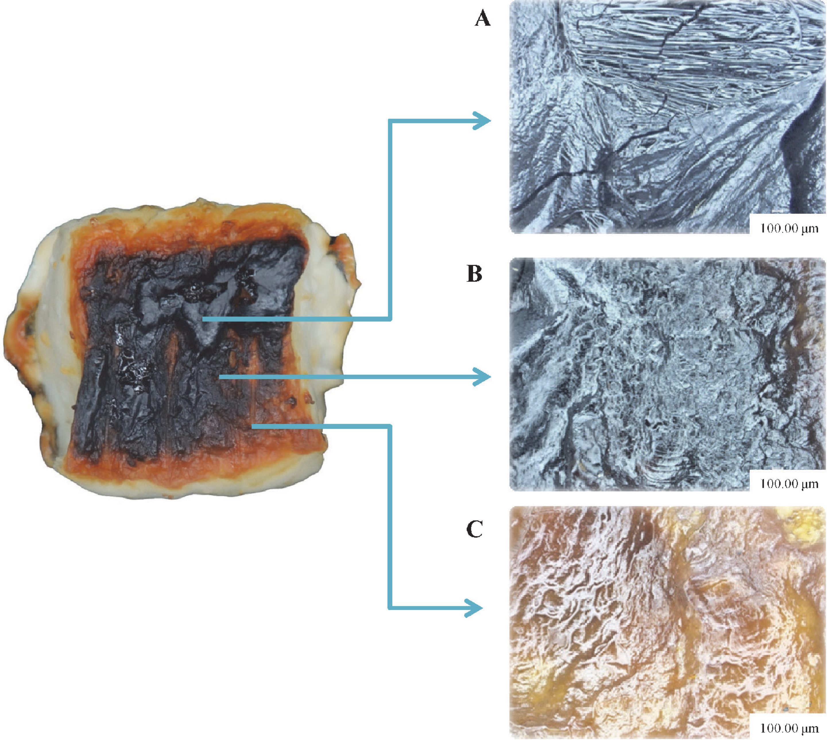
Typical surface structures of grilled fish observed after 30 min of FIR grilling
Estimation of color changes of the fish sample surfaces The carbonization kinetic model is based on the gradual change from substance P to C, as shown in Eq. (1), which shows the formation of high molecular weight (HMW) melanoidins, as colored products that are formed by the polymerization of low molecular weight (LMW) melanoidins. LMW melanoidins are Maillard reaction intermediates, such as furans, pyrroles, pyrrolopyrroles, and/or their derivatives, in the later stage of the reaction (Hayase et al., 2006).
As shown in Fig. 4, the data after browning (at temperatures > 150°C) are plotted to compare the trajectory of color changes because the grilling induces the carbonization in the last step. Two-dimensional projection drawings of the a*-L*, b*-L*, and b*-a* planes are shown in these figures, and the correlations of the measured color values are plotted along with the calculated color values, shown by a solid black line. To estimate the values of a*c and b*c, the following two empirical equations were used:
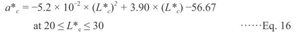 |
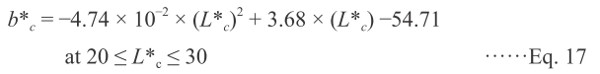 |
where L*c was obtained from the Ea (3.7 ± 0.02 KJ mol−1) and Z (3.91E-1 ± 0.0003 min−1) of the reduction rate of the L* values of red sea bream during the last step of grilling, as controlled by the carbonization.
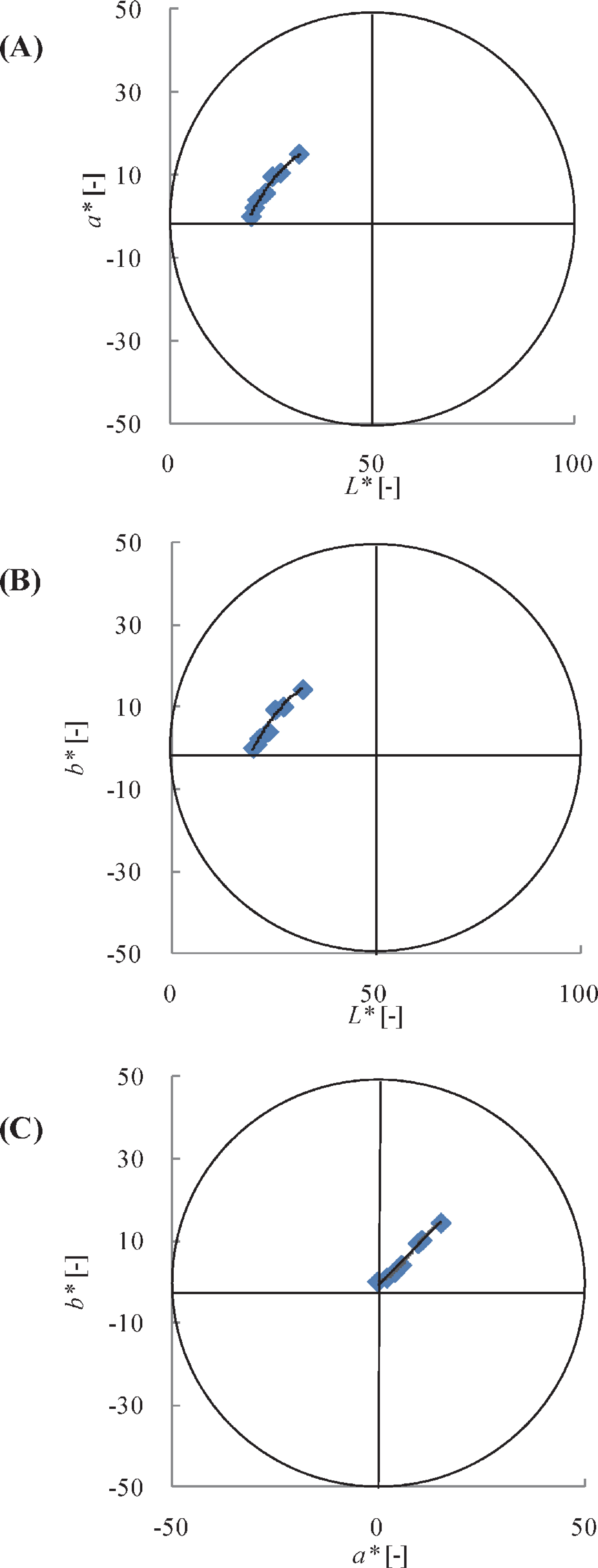
The relationship between a*-L* (A), b*-L* (B), and b*-a* (C). The solid line represents the correlation of the calculated values.
As shown in Fig. 4, a good approximation of the measured data was obtained using the calculated values in all the cases. Thus, when the calculated L*c value decreases, the a*c and b*c values change simultaneously according to Eqs. (16) and (17), respectively. The relationship between the measured values of a* and b* (solid line, Fig. 4C) confirms the results shown in Figs. 4A and 4B. The Ea and Z were found to be extremely smaller than those values of the preliminary steps of grilling (Matsuda et al., 2013; Yu et al., 2014), probably because the kinetic parameters were obtained from the base of the occurrence of browning. Therefore, after the browning is completed, carbonization can occur with very little activation energy. Similar small kinetic parameters were reported by Hosseinpour et al. (2013) for the carbonization step during the drying of shrimp.
As shown in Fig. 5, to estimate the changes in color, the samples were grilled for 30 min, and the results were combined with those reported previously by Yu et al. (2014). Thus, the analysis of the change in color on grilling for longer times extends the scope of the previously reported results obtained for 8 min of grilling. During this stage, the muscle appearance became darker and darker as the surface temperature increased. A gradual reduction of the color profile of L* from 30 to 20 was also observed, a final value at which the L* value seems to reach equilibrium instead of increasing the surface temperature. The color values of a* and b* slightly decreased in a similar rate as the heating proceeded until reaching an equilibrium value of 0. No significant difference (by one-way ANOVA, p > 0.05) was observed between the a* and b* values at this stage. Onishi et al. (2011) reported similar results for white bread during baking. They observed that in the case of baking, the L* value decreased with increasing baking time and appeared to reach a constant value at a certain level depending on the oven air temperature.
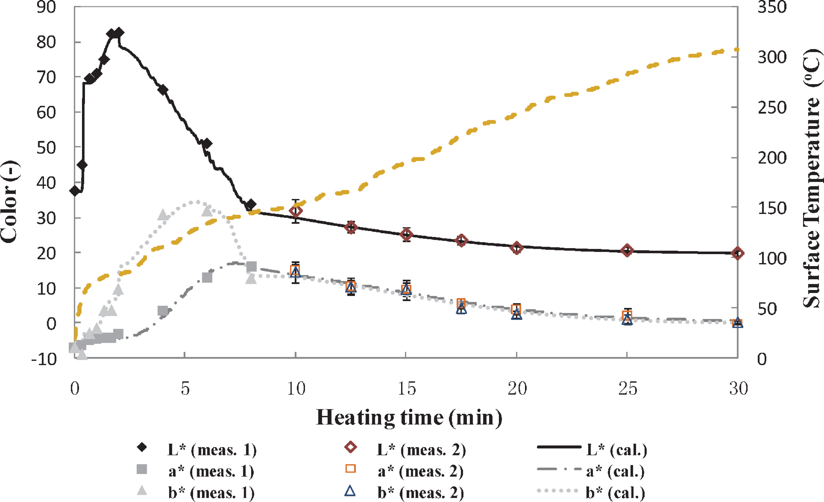
Comparison of calculated and measured L*a*b* values during the entire grilling period. The dashed lines represent the surface temperature profile. The filled dots represent the measured values (1, reported by Yu et al., 2014), and empty dots represent the measured values (2, found in this study).
The relationship between the color changes and surface temperature shows that the carbonization step begins at a temperature close to 150°C. Similar results were reported by Llave et al. (2014b) for the case of Japanese amberjack and red sea bream, Matsuda et al. (2013) using red sea bream, and Wang et al. (2011) for the case of bread, coffee roasted malt, cocoa, and biscuits. Although the reduction in the colors at the carbonization step was not as pronounced as the previous steps, the variable surface temperature process as shown in Fig. 5 confirmed the relevance of surface temperature on the darkening (Fig. 2). Moreover, since carbonization is a subsequent event of browning, and they are continuous during grill processing, it is difficult to strictly divide them into two different parts. Thus, the starting point of this reaction was decided based on the observed abrupt change of the slope of the color profile, especially for the L* value profile.
In addition, as shown in Fig. 5, the calculated L*c, a*c, and b*c values agreed well with the respective measured values. Therefore, when L*c decreases, a*c and b*c change accordingly, even though it was also observed that the heating rate accelerates or decelerates the color changes. Although the color changes during the grilling were successfully estimated by the kinetic model based on the surface temperature measurement and validated with experimental color values obtained using the CDM, it is important to develop a more practical, less time-consuming, and cost-effective method for the analysis of the color changes. Moreover, the CDM provides average values of the color changes of small areas of the sample; thus, many locations must be measured to obtain a representative color profile. Furthermore, the global analysis of the food's surface becomes more difficult. Therefore, a CVS, a potentially fast, non-invasive, and inexpensive method, is a promising tool to solve these problems.
Color analysis using the CVS-calibration Fig. 6 shows the plot of L*a*b* values obtained using the CVS, by the transformation of color space as mentioned above, against the corresponding L*a*b* values measured using the CDM on the tile pattern color sheets. For the camera settings, an f of 5.6 and a shutter speed of 1/40 were observed as the optimal values. The results clearly show a linear relationship obtained with a reasonable fit between the L*a*b* values estimated by the CVS and those obtained using the CDM, with a variance of R2 > 0.97 for all the regression functions.
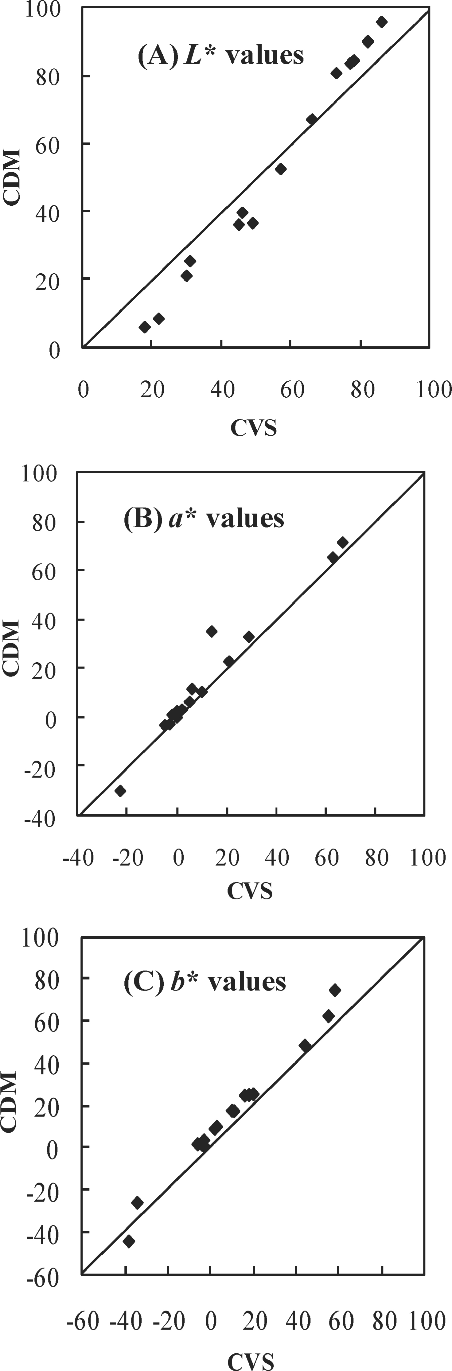
Comparison of the L* (A), a* (B), and b* (C) values obtained by the CVS and CDM of the tile patron color sheets.
Effect of surface temperature on carbonization using the CVS Using the same camera settings defined at the calibration step of the CVS, the effect of temperatures, 160, 180, and 200°C, on the color changes of the sample surfaces was analyzed using the CVS (Fig. 7). Unlike the results shown in Fig. 5; in Fig. 7 the starting point of carbonization under all the conditions was 10 min. At this point, an L* value of 35 was obtained instead of 30. The L* values significantly decreased at high temperatures relative to at low temperatures. However, no significant difference (by one-way ANOVA, p > 0.05) was observed between 180 and 200°C during this step of grilling, thus ending both the processes with an L* value lower than 21. At this precise point, vigorous carbonization on the sample surfaces occurred. In contrast, for the grilling conducted at 160°C, even when the process was allowed to proceed for 30 min, the final L* value decreased to a value just below 27, a point at which the final surface color was not at all black, with some additional brown spots observed at the same time. Additionally, the model has been built based on the knowledge of the initial and final L* values obtained from a specific thermal schedule, which caused the difference in the profile of the color. Thus, these parameters govern the final point at which the model simulated the reduction in the L* value. Although the observed final L* values, which were below 30 in all cases, lead us to believe that carbonization was completed, the results in Fig. 7 confirmed that in order to obtain the charred condition, it is necessary for temperatures to be above 180°C to complete the carbonization of fish samples during grilling under the conditions explained here.
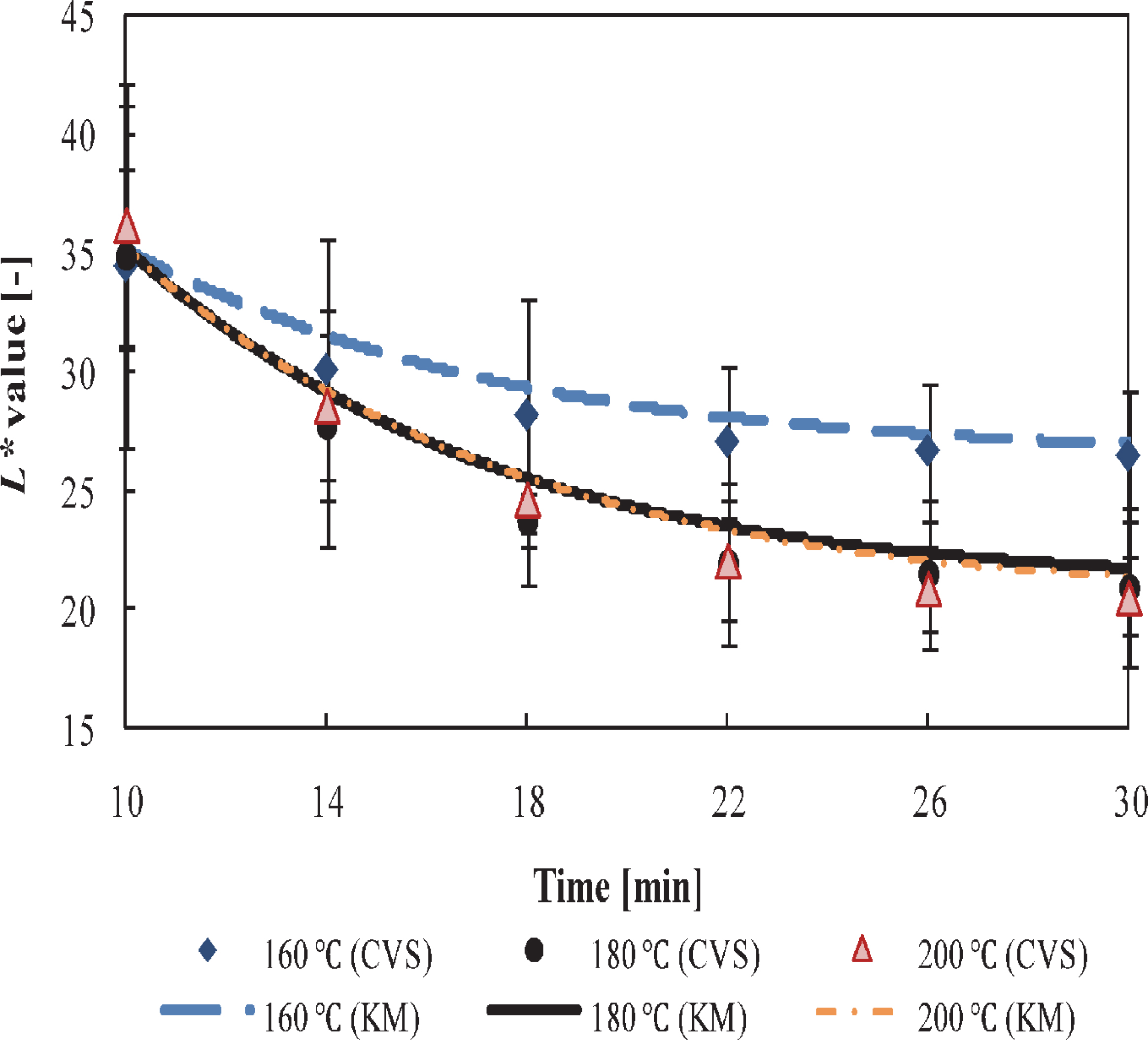
Changes in L* values during carbonization. Color profiles obtained using the computer vision system (CVS) and kinetics model (KM).
The use of higher grilling temperatures provided more energy available for the Maillard reaction, and thus the color degradation was accelerated. Similar results were obtained by Hosseinpour et al. (2013) for drying shrimp. Most of the microscopic structures obtained with the controlled surface temperature of 160°C (not shown), showed a structure similar to “C” in Fig. 3. This confirmed the effect of heating temperature on the surface structure and color changes, providing a reason to maintain the surface temperature as low as possible during grilling.
Fig. 7 also shows a comparison of the estimated values obtained by the CVS and kinetic model (KM). The results are in good agreement even though the surface temperature profiles were different to that used for estimating the kinetic parameters. In addition, the results were also compared to the measured values obtained using the CDM at certain steps. Thus, for example, at the end of the grilling (30 min), no significant difference (by one-way ANOVA, p > 0.05) was observed at high surface temperatures (180 and 200°C) between the CVS and CDM measurements and between both the grilling temperatures on the final L* values; however, at a low surface temperature (160°C), a very small difference of 3.5 ± 1.1°C (mean ± standard deviation) was observed between the CVS and CDM measurements. Iyota et al. (2013) using sliced bread, reported that from the color measurements aspects, the acceptable color difference will be less than 5, because 5 in the L*a*b* system is equivalent to 0.5 in the Munsell color system, which is a commonly used system for the visual evaluation of color. These results justified the use of a CVS for determining the surface color changes during grilling.
Estimation of surface color distribution using the CVS To account for the all-round distribution of color on the surface at each time interval, a CVS technique was employed at different time intervals during the FIR grilling of red sea bream (Fig. 8) using the variable surface temperature process. The distribution in the ranges of the L* values gradually moved towards lower values according to the progress in the grilling time, thus confirming that the surface first browns and then blackens as it burns gradually. Moreover, after a grilling time of 18 min, the maximum L* values in all the time intervals were in the range 0 – 20.
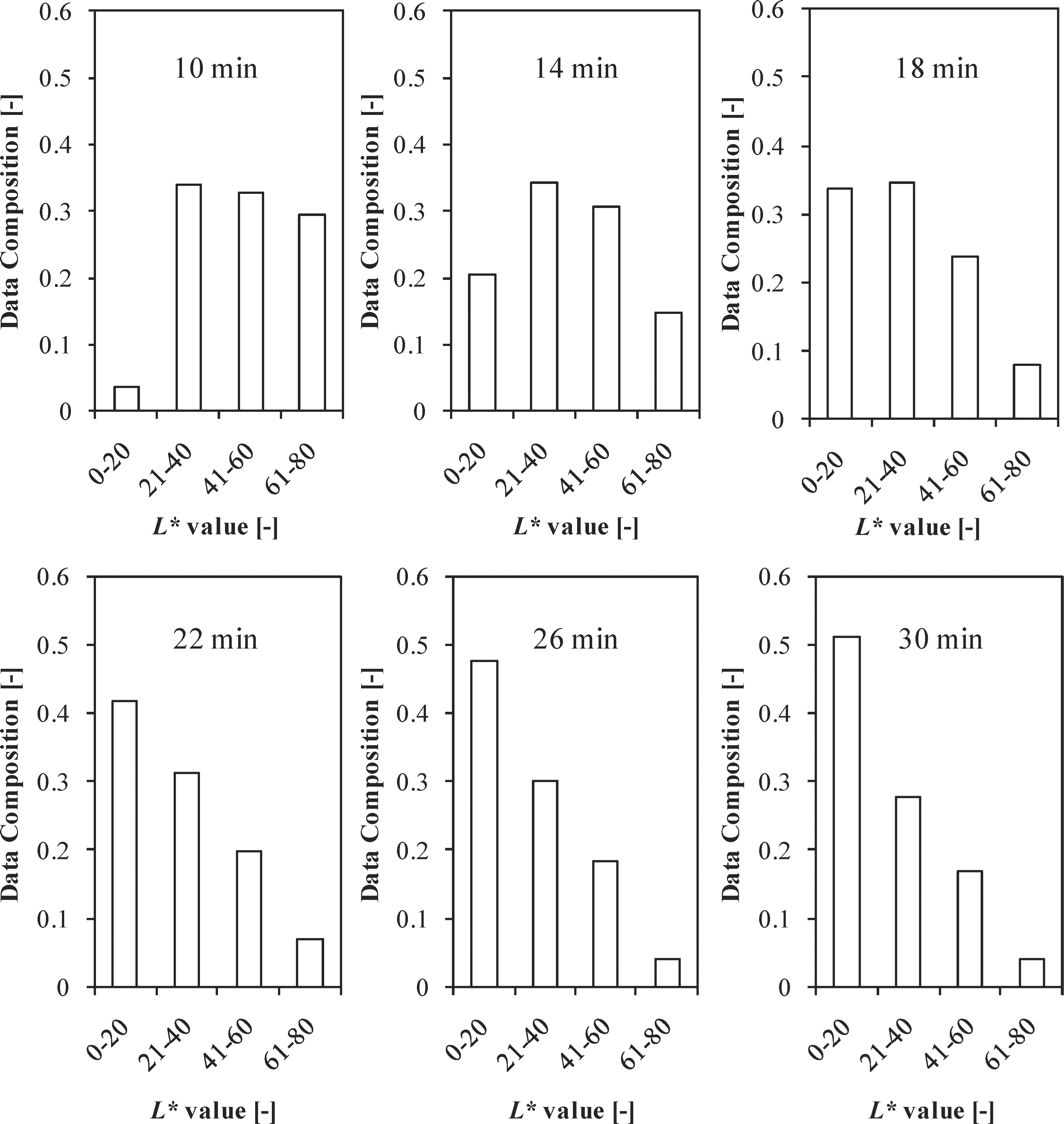
Comparison of the surface distributions of the L* values of red sea bream at several grilling times during the carbonization step.
Simulation of carbonization by the 2D visualization model To visualize the browning and darkening on the sample surface at the end of grilling, the method described by Llave et al. (2014b) was used to extend the grilling time to observe the initial occurrence of carbonization as shown in Fig. 9. The model used the R′G′B′ values obtained from the L*a*b* values by a sequential mathematical transformation using intermediate color spaces. These L*a*b* values were previously predicted by the browning and carbonization kinetic models based on a single measurement of the surface temperature profile at the center during grilling. An empirical equation was used to estimate the temperature distribution of the entire upper surface. To understand the non-uniform browning of red sea bream, mathematical noise functions were included to fine-tune the corrections in the temperature distribution. Finally, the FEMAP software was used to build a 2D model and simulate the browning and darkening with the increase in the temperature during grilling.

Visualization of browning and darkening of red sea bream during FIR grilling using the 2D model and comparison to photographs at the same time step. The variable surface temperature process (A) and the process with a surface temperature controlled at 160 °C (B).
The results show a good approximation of the model in the photographs at any time interval. The non-uniformity of the surface color observed before 20 min was satisfactorily simulated by the 2D model. After 20 min of using process A, a uniform black color formed on the surfaces. The comparison of results between the A and B processes confirms the effect of temperature on color formation during grilling. The process in which the surface temperature was maintained as low as 160°C and a sudden rise in temperature was avoided shows reduced carbonization even for a process time of up to 30 min.
Browning of food occurs at low levels of available water; therefore, it is common during the process of grilling in which the surface layer is dehydrated. Sustained heating of dry surfaces leads to carbonization and is usually accompanied by the generation of smoke. In such circumstances, the food surface first turns browns, following which it blackens as it burns. This study analyzed the effect of surface temperature on the color changes during the last step of grilling. Carbonization was estimated using a kinetic model and CVS. A 2D visualization model successfully simulated the darkening. The results confirm that the darkening was reduced by grilling at a low surface temperature. The use of this practical and economical technique and the 2D visualization model may help support process control in the food industry.