Original papers
Numerical Simulation of Gas Exchange in Fresh-keeping Transportation Containers with a Controlled Atmosphere
2016 年 22 巻 4 号 p. 429-441
詳細
2016 年 22 巻 4 号 p. 429-441
Maintaining a suitable gas composition in a transportation container with controlled atmosphere is important. When O2 concentration is below the suitable value, gas exchange is activated to improve O2 concentration. Computational fluid dynamics was used to compute the effects of exhaust valve location, driving speed, and valve diameter on the gas exchange process. Gas exchange time can be reduced by relocating the exhaust valve to a lower area and by improving driving speed and valve diameter. Moreover, running the fan can shorten gas exchange time and enhance the distribution uniformity of the O2 volume fraction in a container. The influence of gas exchange on temperature in the container can be reduced by shortening processing time, but this reduction significantly affects the distribution uniformity of O2 volume fraction. A test was conducted to verify the accuracy of the numerical models. A good agreement was found between the simulation and test values of O2 volume fraction during gas exchange. Results reveal the rules and characteristics of gas exchange in fresh-keeping transportation containers with a controlled atmosphere.
Fruits and vegetables continue to “breathe” after being harvested. A key method to guarantee the quality of fruits and vegetables involves storing such fresh products in a suitable environment. This environment is usually characterized by low temperature, low O2 volume fraction, and high humidity. Researchers have studied the optimization of fresh-keeping systems (Wang and Touber, 1990; Tassou and Xiang, 1998; Nahor et al., 2005; Hoang et al., 2015). The establishment of a controlled atmosphere (CA) is an effective method to prolong the shelf life of products. The maintenance of a suitable O2 concentration is a crucial function of a container with CA. A low level of O2 volume fraction generally facilitates the limitation of bacteria development and restrains the “breathing” of fresh products. However, excessively low O2 concentrations cause the anaerobic respiration of products. Therefore, the decay process is accelerated. To prevent such anaerobic respiration, the CA system must adjust the O2 concentration in a container quickly so as to avoid extremely low O2 concentrations.
A new type of fresh-keeping transportation truck with CA has been designed and constructed; the O2 concentration in the container can be quickly reduced via liquid nitrogen injection (Enli et al., 2012). The container includes cooling, humidifying, and gas-adjusting systems that can change air temperature and composition. When the O2 concentration is lower than the ideal value, the gas exchange system activates, and the O2 concentration consequently improves. However, certain characteristics of the gas exchange process, such as the influence of fan running and exhaust valve location on the process, remain unknown. These characteristics can be beneficial to the optimization of gas exchange systems. Furthermore, the gas exchange process can be affected by driving speed because the difference in the air pressure inside and outside the container is relatively large when the truck is running. An additional area of study is whether extremely low O2 concentrations occur in certain areas.
Fresh-keeping containers include a space for product storage. The cooling rate, airflow field, and packages in such a space are widely studied. Experimental studies on this topic are often time consuming and labor intensive. In investigating airflow in the said space via testing, numerous sensors and products are placed in the space to simulate actual situations. This requirement is often time consuming and costly. In another aspect, the mass and heat transfer process between the environment and products is difficult to describe via measurement alone. Xiaoteng et al. (2011) and Dongxia et al. (2012) experimentally investigated the distribution of temperature and humidity in a fresh-keeping transportation container that measured 2.40 m long, 1.28 m wide, and 1.40 m high. A total of 32 PT100 sensors were installed in the container. Approximately 500 kg of bananas was placed in the container, and temperature distribution was determined over a period of more than two months. However, when trucks are running, recording data is difficult because of possible vibrations.
The development of computers has facilitated the wide use of mathematical models and computational fluid dynamic (CFD) methods to investigate and optimize the performance of fresh-keeping equipment. Specifically, accurate mathematical models have been developed for cold chain investigation (Gottschalk et al., 2007; Laguerre and Flick et al., 2010 & 2015; Laguerre et al., 2012; Hoang et al., 2012; Chong et al., 2013). Compared with mathematical models, CFD methods can obtain a considerable amount of information about airflow in a given space. The results of these methods are presented through many colorful contour maps that provide excellent insights into the airflow transport process. Many studies have explored the optimization of fresh-keeping equipment, and the development of CFD methods has facilitated the establishment of low-cost but effective techniques for modeling heat and mass transfer in cold systems (James et al., 2006). Defraeye et al. (2014) adopted the shear stress transport k-ω model to investigate the forced convective pre-cooling of oranges in a container. Moureh et al. (2004) and Mitoubkiet et al. (2006) investigated air velocity, temperature field, and other parameters in a car body by applying the CFD method in different turbulent models. Such methods have also been utilized in the study of airflows in packages (Delele et al., 2013; Defraeye et al., 2013), thermonebulization fungicide fogging systems (Delele et al., 2012), and humidification of cold stores (Delele et al., 2009). Therefore, the CFD method can solve many problems related to heat and mass transfer in fresh-keeping systems as well as aid in investigating the gas exchange process in containers. In the present study, a far field is incorporated into CFD model to consider the effects of the external environment on the gas exchange process. A 3-D model can be used for this study, but the grid number must be high to guarantee mesh quality. The problem-solving process requires a significant amount of time and computational resources, which hinder the convenient comparison of different parameters and levels. Foster et al. (2006) developed a 2-D model to investigate the performance of a plane jet air curtain that restricts cold room infiltration. Ho et al. (2011) indicated that 3-D models are complex and require extensive computing time, although they can describe the air distribution in a container in detail. They applied 2-D CFD models to study heat and mass transfer in a refrigerated warehouse and in an office (Ho et al., 2011 & 2010). The simulation results they obtained were in good agreement with the measured data. Therefore, given that the container considered in this study is symmetric in structure, a 2-D model can be used instead.
In the present study, a 3-D simulation was performed, and the results were compared with those of a 2-D simulation to verify their accuracy (Ho et al., 2010). Eleven 2-D CFD models were built to investigate the effects of exhaust valve location, driving speed, valve diameter, and other factors on the gas exchange process. Products were regarded as porous media, as is typical in CFD simulations (Delele et al., 2013). A standard k-ε turbulence model and a SIMPLE algorithm were adopted to solve the problems in gas exchange. The obtained results can be used in the design and optimization of containers with CA for fruits and vegetables.
The structure of a fresh-keeping transportation truck with CA is shown in Fig. 1. This truck includes a chassis and a container. The cooling unit and liquid injection system in the container were disregarded in this study to simplify the computational models and limit the computational cost. The products were stacked according to the work of Dongxia et al. (2012) to achieve proper ventilation in the container. The container sizes are as follows: L1 = 4.00 m, L2 = 2.00 m, L3 = 1.80 m, L4 = 0.80 m, L5 = 0.20 m, L6 = 1.60 m, L7 = 0.10 m, L8 = 0.15 m, and L9 = 0.25, 0.90, or 1.55 m. The container enclosure was composed of 0.8 m-thick polyurethane and was covered with 0.01 m-thick stainless steel. The 3-D structure of the container is presented in Fig. 1a. A fan is located on top of the container. When this fan is running, the air in the container flows clockwise; specifically, the air exits the fan outlet and reaches the back of the container. The air then returns to the fan inlet after flowing through the products and other spaces. Two intake valves were installed in top of the front wall of the container, and two exhaust valves on three different locations (shown as different values of L9 in Fig. 1) were positioned on the back wall. The diameter of these valves was 0.05 m. When the O2 volume fraction is lower than the minimum value, the valves are opened, and the air in the container exchanges with the incoming air from the outside. Thus, O2 concentration improves. In this study, we defined the minimum and maximum values of O2 volume fraction at 3% and 5%, respectively. Air velocity was 6 m s−1 in the fan outlet; therefore, the following simulations with the fan running were all under an air velocity of 6 m s−1. Nonetheless, this velocity must be converted into a 2-D value according to the mass-conserving boundary condition in the 2-D simulation. To simulate gas exchange during transportation, a far field was integrated into the model of the external environment. Moreover, driving speed was altered by changing the air velocity in the far field. Litchi is a common fruit in southern China, and it was reported that CA treatment has great effects on maintaining the post-harvest quality of litchi (Mahajan and Goswami, 2004), thus, litchi fruit was chosen as the products.
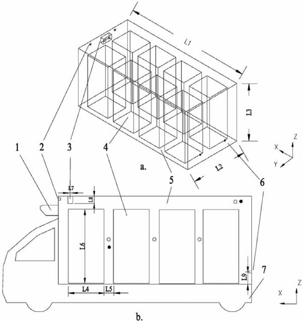
Simplified structure of a fresh-keeping transportation truck with CA
a. 3-D structure b. 2-D model
1. Condenser 2. Inlet valve 3. Fan 4. Products 5. Container 6. Exhaust valve 7. Chassis
Note: ● represents the sensors of the O2 volume fraction, and ○ denotes the temperature and relative humidity sensors.
Certain assumptions were made to simplify the simulation. The air in the container was considered incompressible fluid with constant properties. The gas exchange process was short (less than 30 min); therefore, the effects of product respiration were ignored. Furthermore, the cooling unit and humidifying equipment occupied space in the container, but their effects were ignored as well. The following set of equations describes the mass, momentum, and heat transfer in the models (Anonymous, 2003; Chourasia and Goswami, 2007).
(1) Continuity equation
 |
In each volume unit, mass is factored in, and density changes. The increment in mass should be equal to mass flux density. Buoyancy force increases as a result of density variation according to the assumptions that only the effects of buoyancy term and temperature on fluid density were considered and that other effects were ignored (Ho et al., 2010).
(2) Momentum equation
 |
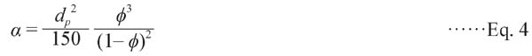
Products affect airflow in a container. In particular, air velocity can be weakened significantly upon coming into contact with products. In this study,  is the fluid body force that mainly includes the drag source term Sj of the porous medium. The effects of products on airflow can be described as follows:
 |
where  is the viscous drag coefficient and C2 is the internal resistance coefficient. α and C2 are described as follows:
 |
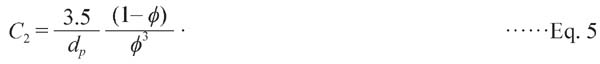 |
In this study, the equivalent diameter of the porous medium (dp) was assumed to be equal to the average diameter of litchi fruits, i.e., 0.03 m. The porosity of the porous medium (ϕ) was calculated according to the package information.
As we discussed in our previous research (Jiaming et al., 2012), the air velocity in the area near the wall of a container is low; thus, wall treatment must be enhanced to consider the effect of wall roughness on airflow. The wall enhancement function can be incorporated into the models by establishing a viscous model.
(3) Energy equation
 |
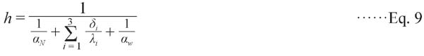
In this model, heat transfer from the external container is integrated by calculating the heat transfer coefficient of the enclosure. Thermal conductivity can be calculated with the following equation:
 |
where θ is the thermal conductivity, density, or specific heat capacity parameter. β is the volume fraction of material 1 in the compound material.
(4) Species transport equation
 |
In this model, the mass originating from products is ignored. Thus, Si is 0. Air is presumably composed of N2, O2, and H2O; these components were set in this study as phases 1 to 3. The governing equations shown subsequently were solved with the finite element method along with the boundary conditions.
The applicable thermal properties of air were obtained from Anonymous (2003). The applicable thermal properties of the container enclosure were derived via calculation. Finally, the applicable thermal properties of litchi products were obtained from the work of Xu (2006), as listed in Table 1. Gravitational acceleration was set as 9.8 m s−2.
| Name | Parameters | Value |
|---|---|---|
| Air | Density/kg m−3 | 1.225 |
| Specific heat capacity/J kg−1 K−1 | 1006 | |
| Heat conductivity coefficient/W·m−1 K−1 | 0.0225 | |
| Dynamic viscosity coefficient | 1 .79×10−5 | |
| Stainless steel plate and polyurethane | Density/ kg · m−3 | 1,612 |
| Specific heat capacity/J kg−1 K−1 | 2,004.44 | |
| Heat conductivity coefficient /W m−1 K−1 | 0.05 | |
| Litchi products | Density/kg m−3 | 932.89 |
| Specific heat capacity/J kg−1 K−1 | 3,710 | |
| Heat conductivity coefficient/W m−1 K−1 | 0.51 | |
| Porosity | 0.3 |
To define the problem accurately, appropriate boundary conditions must be established in this model. Two computational inlets were considered: the far field inlet and the fan outlet. Velocity was constant in both inlets as per the boundary condition for Eqs. 1 and 2. The velocity in the inlet boundary can be set as υx=V, υy=υz=0.
To maintain the relativity of the 2-D model to the 3-D model, V should be calculated on the basis of Eq. 1. In the product space, V was affected by the resistances of the products and their packages. These resistances were calculated using Eqs. 4 and 5. The heat transfer across energy boundaries was considered a surface-to-surface transfer process. The heat transfer coefficient of the wall surface can be calculated with Eq. 9.
 |
The geometry of this model was constructed with AutoCAD. This geometry included a chassis, a container, and a far field measuring 15 m long and 6.5 m high. Then, the geometry was imported into ICEMCFD. The unstructured grid method was used to generate a mixed quadrilateral mesh in a regular area. A triangular mesh was used because of the irregular areas. For instance, the product area was dominated by a quadrilateral mesh. In the transition area between the fan and the intake valve, a triangular mesh was used to limit mesh deformation. To enhance the details in the simulation of these components, mesh density was improved in areas such as the intake valve, exhaust valve, and fan. Reynoldsnumber (Re) (Vali et al., 2015) is an important parameter for simulation; in this study, this variable was calculated with Eq. 10 (Zhu et al., 2010). The largest mesh was 0.05 m, whereas the smallest was 0.001 m. Research on 2-D mesh independence was completed, and the result is shown in Fig. 2, which shows only a 3.1% reduction in maximum velocity (the 16 points in Fig. 3) when the mesh number is reduced from 400,000 to 200,000. A 3-D mesh file (5624300 cells) and five 2-D mesh files were constructed for this research (227715, 228066, 226555, 223000, and 224037 cells), and all equations for this simulation were solved using the finite element method.
 |
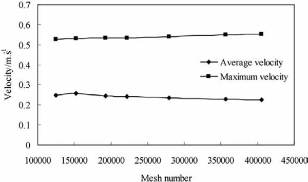
Results of mesh independence study
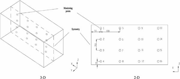
Monitor point locations in the 3-D and 2-D models (unit: cm)
| Simulation# | Valve diameter/cm | Exhaust valve location/cm | Speed/km·h−1 | Fan functioning | Loaded or empty | Modeling dimension |
|---|---|---|---|---|---|---|
| 1 | 5 | 25 | 0 | Yes | Loaded | 3-D |
| 2 | 5 | 25 | 0 | Yes | Loaded | 2-D |
| 3 | 5 | 25 | 45 | Yes | Loaded | 2-D |
| 4 | 5 | 25 | 90 | Yes | Loaded | 2-D |
| 5 | 5 | 90 | 45 | Yes | Loaded | 2-D |
| 6 | 5 | 155 | 45 | Yes | Loaded | 2-D |
| 7 | 10 | 25 | 45 | Yes | Loaded | 2-D |
| 8 | 15 | 25 | 45 | Yes | Loaded | 2-D |
| 9 | 5 | 25 | 0 | No | Loaded | 2-D |
| 10 | 5 | 25 | 45 | No | Loaded | 2-D |
| 11 | 5 | 25 | 90 | No | Loaded | 2-D |
| 12 | 5 | 25 | 0 | Yes | Empty | 2-D |
Twelve simulation cases solved via Fluent are summarized in Table 3. In previous CFD studies on refrigerated food application, the k-ε turbulent model was widely used to solve many turbulence problems with high Reynolds numbers. A standard k-ε model is adequately accurate for the simulations in the present work. This model can also reduce the load of the central processing unit (CPU) and calculation time. In addition, the excellent fault tolerance of this model can address the transition of air between the far field and the container because velocity varies significantly in the calculation area. Therefore, a standard k-ε model was applied in this study. In this model, turbulence intensity (I) was calculated with Eq. 11 (Zhu et al., 2010).
 |
| Conditions | O2 volume fraction/% | Temperature/°C | Relative humidity/% RH | |||
|---|---|---|---|---|---|---|
| Inside | Outside | Inside | Outside | Inside | Outside | |
| Test preparation | 20.9 | 20.9 | 10 ± 1 | 28 ± 1 | 70 ± 5 | 70 ± 5 |
| Test and simulation initialization | 3 ± 0.1 | 20.9 | 5 ± 1 | 28 ± 1 | 50 ± 5 | 70 ± 5 |
First-order implicit transient formulation was implemented as well. A SIMPLE algorithm was used in pressure-velocity coupling. A least squares cell-based method was used in gradient computation. Standard discretization schemes were implemented for pressure computation. First-order upwind discretization schemes were applied to the calculation of momentum, turbulent kinetic energy, and turbulent dissipation rate. The radiation from outside the container was determined using Eq. 9.
When the truck is running, external airflow is turbulent. Airflow is thus difficult to initialize in the cases. Therefore, a steady solver was used to initialize the case. An unsteady solver was then used to simulate the gas exchange process. This model also considers the effects of buoyancy force, as in Eq. 6. The initialization temperature and volume fraction of O2 outside the container was set as 303.15 K and 20.9%, respectively. The corresponding values inside the container were 278.15 K and 3.0%. The natural acceleration attributed to gravity was set to 9.8 m s−2, and the time step was 0.001 s. This time step gradually increased to 5 s. Finally, the calculation process was terminated as soon as the O2 volume fraction reached 5%. This volume fraction was not uniform in the container once exchange valves were closed. Thus, if O2 volume fraction is monitored in only one position, then the average volume fraction might be either greater or smaller than the desired set volume fraction. In this study, the average O2 volume fraction in the container was applied to estimate the end of such simulations. The simulations were conducted using a computer running 64-bit Windows 7 with an Intel® CoreTM 2 i5 CPU and 4GB RAM.
To verify the accuracy of the models, a 3-D model was built, and a test was conducted. Sixteen monitor points were selected on symmetric plane of the 3-D model, and their locations are shown in Fig. 3. In this study, the 3-D model (simulation 1) and 2-D model (simulation 2) were solved with a steady solver. After the simulations were convergent, the velocity values in the certain points were analyzed. The comparison of the velocity distribution in the container between the 3-D model and the 2-D model is shown in Fig. 4. The air velocity in the top areas is greater than those in other areas. In fact, the value of a point in a 2-D model should be equal to the average value of the line with the same x and z locations in a 3-D model in the y-horizontal direction. The velocity distribution in 2-D is in good agreement with the result in the 3-D model. Hence, the 2-D simulations could provide the correct information about the airflow in the container. The difference between these simulations may be due to the mesh number and products (Ho et al., 2010). Thus, in the other simulations, a 2-D model was used.
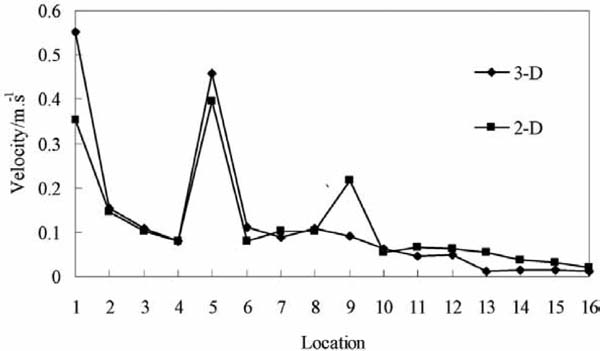
Velocity distribution in the 3-D model (simulation 1) and 2-D model (simulation 2)
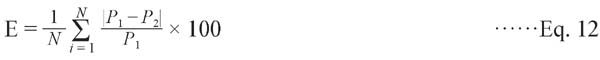
The validation test was conducted on a fresh-keeping transportation container with CA for fruits and vegetables. This test served to verify the accuracy of the simulation models. To negate the factor of vibration, the truck in the test was stopped so that the experimental condition was similar to that in simulation 12 (2-D), as listed in Table 3. To enhance test accuracy, two O2 volume fraction sensors as well as four temperature and humidity sensors were installed, as shown in Fig. 1. The version, measuring range, and other information of these sensors are provided in Table 4. The sensors were connected to a data recording instrument, and data were collected every minute. Before the test, the door of the container was opened until the O2 volume fractions inside and outside the container were almost equalized. Then, the door was closed, and the container was cooled down. Afterward, liquid nitrogen was injected into the container to reduce the concentration of O2, during which the exhaust valve and inlet valve were opened to avoid extremely high pressure in the container. When the average O2 volume fraction in the container was 3%, the injection process was terminated. Next, gas exchange was activated once the O2 volume fraction and temperature were steady. The conditions during the process were recorded until the average volume fraction of O2 reached 5%. All of the instruments were then turned off to end the gas exchange. This test was repeated three times, and the obtained data were averaged. The average value of oxygen concentration was used for comparison. The comparison of the test and simulation results (from simulation No. 12) is shown in Fig. 5. The prediction errors in average temperature and average oxygen concentration were 3.6% and 3.3%, respectively; these values were calculated with Eq. 12 (Delele et al., 2013a). The test and simulation values were in good agreement. Hence, such models exhibited a certain degree of accuracy. Moreover, an empty container requires approximately 18 min to increase O2 volume fraction from 3% to 5%.
 |
| Sensor | Version | Measuring range | Accuracy |
|---|---|---|---|
| O2 volume fraction | EC810 | 0% to 25% | ±0.7% |
| Temperature | CHT-D | −20°C to 80°C | ±0.3°C |
| Relative humidity | CHT-D | 0% to 100% RH | ±3% RH |

Comparison of experimental values and simulation values
a. Average temperature; b. Average oxygen volume fraction.
where E is the prediction error, N is the number of samples, P1 is the measured value, and P2 is the prediction value.
The solution of air velocity and the distribution of the O2 volume fraction for simulation 2 are shown in Fig. 6. The velocity distribution in the far field and in the container are shown in Fig. 6a. When the truck was running at 45 km h−1, the air velocity in the far field inlet was approximately 12.5 m s−1, whereas that at the top region outside the container reached roughly 24 m s−1; the air velocity behind the truck was below 2 m s−1.
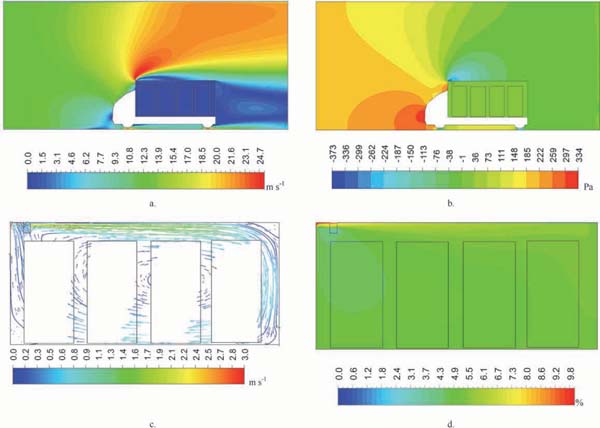
Airflow distribution within and outside the container (simulation 3)
a. Air velocity distribution within and outside the container; b. Pressure distribution in the container; c. Air velocity vectors in the container; d. O2 volume fraction distribution in the container.
Air pressure distribution is depicted in Fig. 6b. With the truck running, it provided a lift force to the air such that a negative pressure behind the container was noted. The air pressure in front of the truck was stronger than that behind the container by more than 300 Pa. The distribution of air velocity vectors in the container is indicated in Fig. 6c. The figure shows an eddy in the middle of the container. The running of the fan accelerated the air circulation and facilitated a clockwise airflow. Air from the outside entered the container and mixed with the air inside before proceeding to the back areas. A relatively low air velocity was observed in the middle and in the back of the container. The air velocity in the exhaust valve was lower than that in the intake valve. The distribution of O2 volume fraction in the container at the end of the gas exchange is shown in Fig. 6d. As shown in Fig. 6c, the O2 volume fraction of the air outside was high (20.9%); the O2 volume fraction was particularly high in the front and top areas of the container.
Gas exchange time The effects of exhaust valve location on the exchange time for simulations 3, 5, and 6 are detailed in Fig. 7a. In these simulations, the driving speed was 45 km h−1, and the fan was running. The effects of different exhaust valve locations were not significant (P > 0.05) in the first 30 s. Subsequently, the difference in the O2 volume fractions among various exhaust valve locations increased. When L9 = 155 cm, the duration of the exchange process was maximized at 220 s. When L9 = 25 cm, however, exchange time was minimized at 135 s.
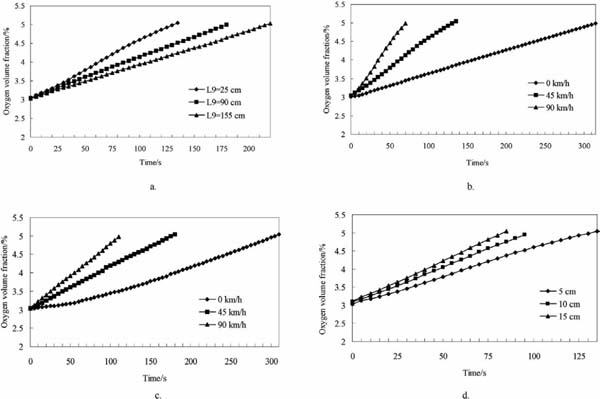
Effects of different factors on changes in O2 volume fraction in the container
a. Effects of exhaust valve location; b. Effects of driving speed; c. Effects of driving speed without fan running; d. Effects of valve diameter.
The effects of different driving speeds on gas exchange time are shown in Fig. 7b. The data were derived from simulations 2 to 4. When L9 = 25 cm, the fan was running, and the driving speed was 90 km h−1; the process of increasing the O2 volume fraction from 3% to 5% required only 70 s. When the truck stopped, the exchange time increased to 315 s in the absence of a significant pressure difference in the air inside and outside the container when the truck was running (shown in Fig. 6b). The effects of driving speed on the gas exchange process without the fan running are shown in Fig. 7c. The data originated from simulations 9 to 11. The gas exchange speed was relatively slow in the first 60s. Subsequently, this O2 volume fraction began to improve quickly, and the O2 volume fraction in the container reached 5%; such improvement required approximately 120 s more than that required when the driving speed was 45 km h−1. When the driving speed was 90 km h−1, the O2 exchange time was approximately 110 s. This time was considerably longer than the gas exchange time when the fan was running.
The effects of valve diameter on gas exchange time are shown in Fig. 7d. The data originated from simulations 3, 7, and 8. When the driving speed was 45 km h−1 with the fan running, the valve diameter was 15 cm, and the gas exchange time was 85 s. This duration was shorter than the exchange times of the other two diameter levels. When the valve diameter was 5 cm, the O2 volume fraction in the container increased from 3% to 5 % in 135 s. When the valve diameter was 10 cm, the gas exchange time was roughly 10 s shorter than that at 5 cm.
Uniformity of gas volume fraction in the container To understand the variation in the distribution of the O2 volume fraction in the container, the average values of the O2 volume fraction on equal distance lines (Ho et al., 2011) in the container were analyzed. Furthermore, the standard deviation of the entire container was calculated by
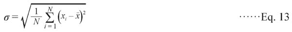 |
where σ is the standard deviation, xi is the average O2 volume fraction of No. i line, and x is the average O2 volume fraction of the whole container. The distribution of the data lines is illustrated in Fig. 8. The effects of different exhaust valve locations on O2 volume fraction distribution are shown in lists 3, 5 and 6 in Table 5. The difference among the standard deviations was 0.04. Moreover, the standard deviation was minimized at 0.47 when L9 = 155 cm. The standard deviations of different driving speeds are presented in lists 2, 3, and 4 in Table 5. When the driving speed was 90 km h−1, the standard deviation decreased, and the maximum O2 volume fraction was 5.37%. The distribution of the O2 volume fraction was relatively uniform in all cases. The effects of different valve diameters on standard deviation are shown in lists 3, 7, and 8 in Table 5. Standard deviation was high when the valve diameter was large, and the maximum standard deviation was 0.89 while the maximum O2 volume fraction was 7.64%. The effects of driving speeds on standard deviation when the fan was not running are provided in lists 9 to 11 in Table 5. The difference in the distribution of the O2 volume fraction was small at a high driving speed. Specifically, the standard deviation was 1.09 when the truck was stationary, and the maximum O2 volume fraction was 8.67%. The average standard deviation across the three simulations was 0.30 when the fan was running. By contrast, this average was 0.70 without the fan running.
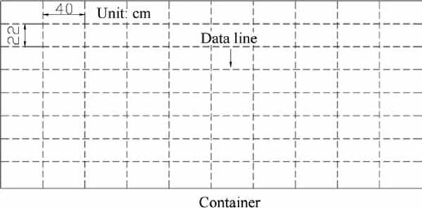
Distribution of data lines
| Simulation# | 2 | 3 | 4 | 5 | 6 | 7 | 8 | 9 | 10 | 11 |
|---|---|---|---|---|---|---|---|---|---|---|
| Minimum value /% | 4.97 | 4.74 | 4.67 | 4.02 | 4.43 | 3.85 | 3.77 | 4.32 | 4.14 | 4.33 |
| Maximum value /% | 5.98 | 7.17 | 5.37 | 6.49 | 6.95 | 6.93 | 7.64 | 8.67 | 6.88 | 6.77 |
| Standard deviation | 0.22 | 0.48 | 0.20 | 0.51 | 0.47 | 0.66 | 0.89 | 1.09 | 0.55 | 0.47 |
Product temperature The change in average temperature in the container during the gas exchange in simulation 3 is shown in Fig. 9. In the initial stage, the average temperature in the container increased from 5°C to 6.5°C in 20 s. Then, the speed of this rise decreased, and in the end, the product temperature rose to roughly 7°C. The fluctuations in air temperature were obvious in the gap between the products and the container wall during the gas exchange. By contrast, product temperature was relatively stable because of the high specific heat capacity.
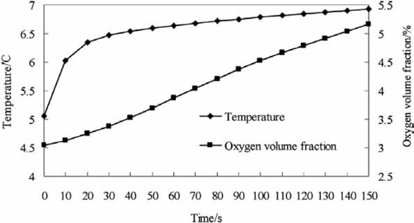
Changes in temperature and O2 volume fraction during gas exchange
The temperature distribution in the container during the gas exchange in simulation 3 is shown in Fig. 10. The gas exchange process also affected product temperature by increasing the temperature in the top and back areas, as suggested in Figs. 10a to 10c. Hot air accumulated in the back areas of the container. The depth from the surface to the center of the products, in which temperature was affected, was roughly 20 cm at the end of the gas exchange.
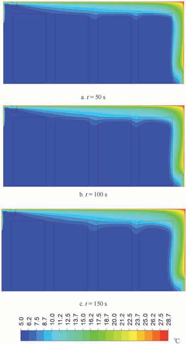
Change in temperature distribution during gas exchange
CFD simulation has been widely used in the description and design of post-harvest facilities, including products and packaging (Defraeye et al., 2014; Delele et al., 2013a, b; Ferrua and Singh, 2009), storage facilities (Chourasia et al., 2007; Delele et al., 2009; Foster et al., 2006), and refrigerated transport (Moureh et al., 2009a, b; Tapsoba et al., 2007). This study addresses the optimization of the gas exchange system for transportation with CA. Thus, a 2-D model was used to predict the influence of exhaust valve location, driving speed, and diameter of valve on gas exchange performance. To improve the airflow patterns in a ventilated enclosure, a 3-D model is useful to obtain considerable data in only one case (Foster et al., 2006; Tapsoba et al., 2007). However, in this study, the outside fluid conditions were investigated, and a far field containing numerous meshes in the 3-D model was built. Meanwhile, the solutions of 3-D models require considerably more computing time than those of 2-D models, especially when achieving comparisons among many cases. Twelve cases were used in this study, and many comparisons were needed. Thus, a 2-D model was ultimately selected.
Model verification Ho et al. (2011) used 2-D and 3-D models to investigate airflow in a warehouse and proved that 2-D models can describe flow information as effectively as 3-D models can. In the present study, although the container and the devices in it were symmetric in the y- direction, the fan was not as wide as the container; the flow rate and velocity should thus be adjusted on the basis of the width of the fan and that of the container. To verify the model result, a 3-D model was built, and the results matched the 2-D model results. Hence, the method is accurate for changing complex geometry from 3-D to 2-D. With this approach, the cost to study post-harvest storage facilities can be reduced. As shown in Fig. 4 and Eq. 10, the air turbulence was higher in the front than in the back areas of the container. This result is in agreement with that of Tapsoba et al. (2007). Concurrently, a test was built according to one of the cases. In this test, the results were compared with the results from the simulation. Temperature (Dehghannya et al., 2011; Delele et al., 2013a; Tutar et al., 2009) and velocity (Moureh et al., 2009) are common indexes for verification. In the present study, temperature and oxygen concentration variation were verified.
Performance analysis of gas exchange The airflow patterns in the outside environment of a truck are difficult to measure when the truck is running. However, with the CFD method, an overall view can be achieved by solving the far field computational domain, as shown in Fig. 6. The far field can be used in the study of post-harvest storage facilities (Foster et al., 2007), as well as in the design of trucks (Xiaoni and Yongqi, 2011; Xingjun et al., 2014), aerospace (Huixue et al., 2010; Suresh et al., 2015), and architecture (Ai and Mak, 2014). The high resistance in front of a container improves the fuel cost of the truck; a guide plate may help reduce resistance. During the gas exchange process in this study, the entry of air from the outside and its exit from the inside were accelerated by the joint effects of the pressure difference between the inside and outside environments, as seen in Fig. 6b. Such a result indicates that truck running is beneficial for gas exchange. Given the drag force caused by the fan running and the lift force from product surfaces (Mclaughlin, 1989), the gravity effect on airflow is not significant (Delele et al., 2012). Significant turbulence was observed in the front areas of the container because of the high-velocity air in the x-direction from the fan mixing with the airflow returning from the back areas; such a phenomenon was called the “ceiling Coanda effect” by Tapsoba et al. (2007). The large eddy in Fig. 6c can be enlarged by improving the air velocity in the fan outlet; these airflow patterns explain that oxygen concentration was higher in the back areas than in the front areas, as shown in Fig. 6d.
Gas exchange time Changing exhaust valve locations can change the airflow route during gas exchange, as shown in Fig. 6c. Similar to choosing the location of a window for a room (Ai and Mark, 2014; Bangalee et al., 2014; Parto and Palizi, 2012), changing the location of the exhaust valve significantly affects gas exchange. In this study, the lower location of the exhaust valve was proved to be helpful to improve gas exchange efficiency, as shown in Fig. 7a. This finding may be ascribed to the fact that when the exhaust valve was located in a higher place, the gas exchange route was shortened in z- direction that most of the air flowed in x-direction as the effect of gravity was not significant. This situation does not benefit the mixing of external air with that in the container. Efficiency is reduced as air enters the container without mixing fully with the air inside before exiting from the exhaust valve. Thus, the gas exchange process is long when the exhaust valve is in a high position.
Exchange efficiency can therefore be improved when the truck is running, given that gas exchange time can be reduced with high driving speed. When the truck is stationary (driving speed of 0 km h−1) and in the absence of a running fan, the gas exchange process is mainly driven by buoyancy (Boulard et al., 2002). The diffusion force from natural convection (Parto and Palizi, 2012) is relatively small in such areas. Therefore, the exchange process is relatively long. After outside air enters the container, it diffuses via convection, which is driven by O2 concentration and temperature gradients (Delele et al., 2012). Thus, the oxygen concentration in the container grows rapidly after only 60s. Warm air with high O2 volume fraction needs a relatively long time to enter the container without the fan running. The comparison between the conditions in which the fan is running and not running (Figs. 7b and 7c, respectively) indicates that fan running affects gas exchange time to a certain degree, especially when the driving speed is relatively high.
Valve diameter significantly affects gas exchange time, that is, a high valve diameter can be helpful in shortening gas exchange time, as shown in Fig. 7d. Dehghannya et al. (2011) also showed that a large vent area for packages can improve the forced convection cooling of produce. This phenomenon accounts for the cross-sectional area of gas exchange being improved when the valve diameter is large; such an improvement reduces ventilation resistance and improves gas exchange efficiency. However, the best valve diameter should be determined according to container volume and length.
Uniformity of gas volume fraction in the container and produce temperature Although airflow tends to be uniform through natural convection after gas exchange in the container, limiting the variation of O2 volume fraction in the container can decrease self-regulation time, which is beneficial for energy saving. This limitation can prevent physical defects in fresh products caused by environmental fluctuations. After the analysis of the standard deviation of the oxygen concentration distribution in this study, the minimum standard deviation was found to be 0.20, whereas the maximum was found to be 1.09. This result indicates that fan running can reduce the standard deviation of O2 volume fraction distribution and improve distribution uniformity (Delele et al., 2012). A large container may equate to a high standard deviation and air turbulence deviation; many eddies can also be seen (Moureh et al., 2009a; Tapsoba et al., 2007).
Temperature is the most important factor that influences the quality of fresh products because respiration rate is relatively low in low temperature conditions (Rezagah et al., 2014). Thus, reducing the fluctuation of temperature can prolong the shelf life of fresh products. The effects of gas exchange on temperature in the container should be minimal during the exchange process.
When the container is full of products, the available space for air is limited such that the flow resistance of products increases; air enters the container and reaches the back areas. The air mainly passes through the gap between the container wall and the products at the top and back areas; thus, the temperature in such areas is higher than those in other areas. Therefore, fluctuation in air temperature is obvious in the gap between products and the container wall during gas exchange. Product temperature is relatively stable because of the high specific heat capacity.
The result shown in Fig. 10 indicates that gas exchange can influence the temperature of products. Reducing gas exchange time can limit this effect; however, such a reduction may improve the standard deviation of O2 volume fraction distribution.
Finally, the results of this work are based on certain assumptions, such as the weather outdoors being agreeable without any wind, the truck running on a smooth road such that the vibration is small and constant, and the effects of humidity on the gas exchange being ignored. The aim of this study, however, is to indicate the performance of the gas exchange system in a container with CA under different conditions. The results will thus be helpful in the design and optimization of gas exchange systems. The assumptions may have considerable effects on the result in some conditions, much specific work is presently being conducted. In addition, numerous factors that may affect the performance of gas exchange are being investigated by our group.
Heat and mass transfer during gas exchange was investigated in this study using a fresh-keeping transportation container with CA. Numerical simulations were conducted to predict and optimize airflow in the container. A test and 3-D simulation were conducted to verify the results of one simulation. The results indicated that the test and simulation values are in good agreement. Thus, the other simulations can also generate useful and reasonably accurate results. Specifically, this study performed 11 2-D simulations to study the effects of exhaust valve location, driving speed, and valve diameter on the gas exchange process. Gas exchange time can be shortened by reducing the height of the exhaust valve, improving driving speed, and increasing valve diameter. The distribution of O2 volume fraction can also be improved with fan running, which also somewhat reduces gas exchange time. Limiting gas exchange time can weaken the effects of the aforementioned factors on temperature in the container. Moreover, this process significantly affects the uniformity of the distribution of O2 volume fraction. The gas exchange process may be influenced by the deviation of temperature inside and outside the container, the stacking methods of products, and container structure.
Acknowledgments The authors acknowledge the financial support from the National Science and Technology Support Program of China (2013BAD19B01-1-3), the Design of Containers with Controlled Atmosphere for Fruits and Vegetables.
fluid density, kg m−3
;%0A%09%09%09newWindow.document.open();%0A%09%09%09newWindow.document.write('<img src=%22./Graphics/22_429_26.jpg%22>');%0A%09%09%09newWindow.document.close();%0A%09%09)
velocity vector, m s−1
ttime, s
pstatic pressure, Pa
;%0A%09%09%09newWindow.document.open();%0A%09%09%09newWindow.document.write('<img src=%22./Graphics/22_429_27.jpg%22>');%0A%09%09%09newWindow.document.close();%0A%09%09)
acceleration due to gravity, N m−3
;%0A%09%09%09newWindow.document.open();%0A%09%09%09newWindow.document.write('<img src=%22./Graphics/22_429_28.jpg%22>');%0A%09%09%09newWindow.document.close();%0A%09%09)
fluid body force, N m−3
µfluid dynamic viscosity, pa s
υjvelocity components in x-, y-, and z- directions, m s−1
αpermeability of porous medium, m2
C2internal resistance coefficient, m−1
dpequivalent diameter of porous medium, m
Effluid energy, J kg−1
Epproduct energy, J kg−1
ϕporosity of porous medium
ρpdensity of porous medium, kg m−3
keffeffective thermal conductivity of porous medium, W m−1 kg−1
Ttemperature, K
hienthalpy of species i, J kg−1
Jidiffusion flux of species i, kg m−2 s−1
Shjsource of energy, W m−3
Sisource of extra mass, kg s−1
Ucharacteristic scale of velocity, m s−1
Vair velocity in fan outlet, m s−1
YiMass fraction of gas component i in air
Lcharacteristic scale of length, m
vkinematic viscosity, m2 s−1
Iturbulence intensity, %
ReReynolds number calculated by hydraulic diameter
θone of the parameters, include thermal conductivity, density and specific heat capacity
βvolume fraction of material 1 in the compound material
hconvective heat transfer coefficient, W m−2 K−1
αNexternal heat transfer coefficient, W m−2 K−1
αwwall surface heat transfer coefficient, W m−2 K−1
λithermal conductivity of enclosure materials i, W m−1 K−1
Δithickness of enclosure materials i, m