Introduction
Yellowtail (Seriola quinqueradiata), with total production of approximately 123,000 t in 2015, is one of the most important fish species reared by aquaculture in Japan. Various food science studies have been conducted on yellowtail, and much work has been done on distinguishing dark muscle (DM) and ordinary muscle (OM). Examination of lipids, K values, extractive components and volatile or flavor components have demonstrated differences in the biochemical composition of DM and OM and that the quality of DM is more significantly reduced than is OM with storage (Murata and Sakaguchi, 1986; Sakaguchi et al., 1982; Sohn et al., 2005, 2007; Tanimoto and Shimoda, 2016).
Relatively large fish such as yellowtail are often divided into sections for consumption, and the OM is further broken down by type as dorsal (DOM), ventral (VOM) and caudal (COM). Fish muscle from these types is often cut into blocks, sliced or minced prior to distribution to the marketplace. When distributed as cuts of fish, it may be difficult even for specialists to distinguish the source type by appearance or taste, making evaluation using objective indicators, such as biochemical indicators, important. VOM has different lipid content than other OMs (Shimizu et al., 1973) and, therefore, can likely be distinguished based on lipid content. However, to date, there are no reports on the differences in biochemical composition between DOM and COM, and these are currently considered to be difficult to distinguish. On the other hand, consumer preference differs depending on the source tissue type of the muscle because taste and texture properties differ. For some species of fish, the muscle tissue from different parts of the body is sold for very different prices; therefore, it is important to develop methods for distinguishing fish muscle by type in order to prevent fraud.
With recent improvements in instrumental analysis and statistical analysis software, comprehensive analysis of metabolic components has become possible (Cevallos-Cevallos et al., 2009). Metabolic analysis utilizing analytical methods, such as nuclear magnetic resonance spectroscopy, gas chromatography-mass spectrometry (GC-MS), liquid chromatography-mass spectrometry and capillary electrophoresis–mass spectrometry, is emerging as a promising method for making quantitative assessments of food products (Pongsuwan et al., 2007; Ramautar et al., 2015; Shiga et al., 2014). These methods allow objective characterization of samples through comprehensive analysis of metabolites. In a bivalve mollusk, Mediterranean mussel (Mytilus galloprovincialis), Aru et al. (2016) clarified the relationship between metabolites and storage and microorganisms. However, there have been only limited applications of metabolic analysis in the field of aquatic food science. To the best of our knowledge, there are no reports of applying metabolomics to distinguishing fish meat by muscle type.
In this study, the goal is to develop a novel method for distinguishing the different types of the fish muscle by GC-MS based on metabolic analysis. Thus, orthogonal partial least squares discriminant analysis (OPLS-DA) using GC-MS data was applied to distinguishing yellowtail muscle types.
Materials and Methods
Experimental samples Experimental samples were prepared as previously reported by Tanimoto et al. (2018). On three occasions, on July 14, September 29 and November 5, 2014, two yellowtail for a total of six fish (mean weight, 5.4 ± 1.2 kg) reared by aquaculture were purchased at a local market in Hiroshima, Japan, killed by ikejime at the market, filleted and transported on ice to the laboratory within 8 h. Fillets of each fish were rinsed with chilled 0.85% saline and then separated into DM and DOM, VOM and COM. About half of the ordinary muscles located dorsally and ventrally to the head was excised for DOM and VOM samples, respectively. COM samples were prepared from about one-third of the fillet located caudally and excluding DM. Muscle samples of the same type from the two fish purchased on the same date were minced together using a food processor (MK-K60P, Panasonic, Japan). The minced fish muscle was wrapped tightly with polyethylene film to prevent the surface from drying. To simulate storage conditions prior to consumption as sashimi (raw sliced fish), the samples were stored at 5 °C for 1 day on a net tray. These samples were then frozen and stored at −80 °C until analysis. Each minced fish muscle sample was freeze-dried (Freeze Dryer FD-5N; EYELA, Japan) and dry-milled (Tube-Mill C S001; IKA, Germany). These samples were stored at −80 °C until analysis.
Sample preparation and derivatization Each fillet sample (n = 3) was analyzed in triplicate. Sample preparation and derivatization was conducted as reported by Pongsuwan et al. (2007) with modification. Hydrophilic primary metabolites in 50 mg of fish meat were extracted using a solvent mixture 1 mL of MeOH/ultrapure water/CHCl3 in a ratio of 2.5/1/1 (v/v/v) with the addition of 60 µL of 0.2 mg/mL ribitol as an internal standard for GC-MS and shaking at 3,000 rpm for 5 min followed by centrifugation at 16,000 × g at 4 °C for 5 min. Then, 400 µL of ultrapure water was added to 800 µL of supernatant in a microtube and shaken at 3,000 rpm for 1 min. Following centrifugation at 16,000 × g at 4 °C for 5 min, 400 µL of aqueous phase was transferred to another microtube, and the remaining organic layer was evaporated using a centrifugal evaporator (CVE-2000; Eyela, Japan) at room temperature for 1 h. Following evaporation, the extract was freeze-dried overnight.
For derivatization, 50 µL of methoxyamine hydrochloride in pyridine (20 mg/mL) was added to each freeze-dried sample, and the mixture was incubated in a dry incubator (Thermo Q, Bioer, China) at 30 °C for 90 min to produce a methoximation reaction (derivatization for C=O). Following the addition of 50 µL of N-methyl-N-(trimethylsilyl) trifluoroacetamide, the reaction mixture was incubated at 37 °C for 90 min to induce the trimethylsilylation reaction (derivatization of functional groups, such as -NH2, and -OH). The derivatized sample was analyzed by GC-MS.
GC-MS analysis Analysis of derivatized metabolic components was performed using a Gas Chromatograph-Mass Spectrometer (GCMS-QP2010, Shimadzu, Japan). GC-MS was conducted as described by Nishiumi et al. (2010). Briefly, 1 µL of derivatized sample was injected in split mode (10:1) into a capillary GC column (Agilent J&W DB-5, Agilent Technologies, USA) via an injection port maintained at 250 °C with helium carrier gas with a linear velocity of 39.0 cm/s and a purge flow of 5 mL/min. The column temperature was held at 100 °C for 4 min, then raised at 10 °C/min to 320 °C and held for 11 min. The MS conditions were as follows: transfer line temperature, 280 °C; ion source temperature, 200 °C. Electron-impact ionization (EI) was used for MS with an ionization voltage of 70 eV. Mass scans were conducted in full scan mode over the range of m/z 45–600 at 2,000 scans/0.3 s.
Data processing Peak detection and calculation of the peak area were conducted using the GC-MS solution software package (Ver. 2.72, Shimadzu). Retention indices of major compounds were calculated against a standard n-alkane mixture (C6-C33). Peak annotation was performed using a commercially available database (GC-MS metabolite database Ver. 2, Shimadzu). The ratio of peak area of a metabolite to that of ribitol was calculated and reported as a semi-quantitative value.
Statistics The data set was prepared as a data list with sample name on the first line, group number on the second line and each compound listed after the third line. Principal component analysis (PCA) and orthogonal partial least squares discriminant analysis (OPLS-DA) were performed using commercially available software (SIMCA 14, MKS Instruments, USA). Pareto scaling was applied to data processing. Data are expressed as the mean ± standard deviation (SD). Significant differences (P < 0.05) of mean values between the two meat groups (i.e., DM vs OM) was subjected to Student's t-test and three OM subgroups (i.e., DOM, VOM and COM) were subjected using the and one-way analysis of variance (ANOVA) followed by Tukey's test, respectively. Analyses were conducted using IBM SPSS Statistics 24 (IBM, USA).
Results and Discussion
GC-MS data acquisition Metabolic components levels in yellowtail muscle were determined from typical total ion current chromatograms (TIC) as shown in supplementary Fig. S1. Peaks were numerous and the patterns did not vary greatly by sampling tissue. In our study, 100 peaks (hereinafter, metabolites) were annotated, and the overall totals were 70 for DM and 92 for OM (Supplementary Table S1). By type in the OM, the number of annotated metabolic components was 64 for DOM, 59 for VOM and 78 for COM. The 100 metabolic components were classified by biochemical composition as follows: 40 sugars, 23 amino acids, 7 organic acid, 5 nucleic acid-related compounds (NARs), 7 phosphorylated compounds, 4 vitamins and 14 others. Table 1 shows the classification of metabolic components in the tissue types of yellowtail muscle. Metabolic components were rich in sugars and amino acids, but there were no large differences among the classification profiles of metabolic components in each tissue type.
Table 1.
Composition of annotated metabolites in tissues by type
| Classification |
Overall muscle |
Dark muscle |
Overall ordinary muscle |
Dorsal ordinary muscle |
Ventral ordinary muscle |
Caudal ordinary muscle |
| Sugar |
40 (40) |
28 (40.0) |
36 (39.1) |
22 (34.4) |
20 (33.9) |
25 (32.1) |
| Amino acid |
23 (23) |
17 (24.3) |
23 (25.0) |
21 (32.8) |
20 (33.9) |
23 (29.5) |
| Organic acid |
7 (7) |
5 (7.1) |
6 (6.5) |
5 (7.8) |
4 (6.8) |
4 (5.1) |
| Nucleic acid-related |
5 (5) |
4 (5.7) |
4 (4.3) |
4 (6.3) |
4 (6.8) |
4 (5.1) |
| Phosphorylated compounds |
7 (7) |
4 (5.7) |
7 (7.6) |
4 (6.3) |
3 (5.1) |
7 (9.0) |
| Vitamin |
4 (4) |
4 (5.7) |
3 (3.3) |
3 (4.7) |
3 (5.1) |
3 (3.8) |
| Other |
14 (14) |
8 (11.4) |
13 (14.1) |
5 (7.8) |
5 (8.5) |
12 (15.4) |
| Total |
100 (100) |
70 (100) |
92 (100) |
64 (100) |
59 (100) |
78 (100) |
Values are the number of metabolites in each tissue for each classification category.
Numbers in parentheses are percentages of each metabolite class for each tissue type.
In metabolic analysis, the target metabolic components available for analysis may depend on extraction method and analytical methods used to collect data. In this study, we were able to identify 100 metabolic components based on extraction of water-soluble primary metabolic components and analysis using GC-MS. This analysis pool was comparable to 53 metabolic components identified from the serum of tiger puffer fish (Takifugu rubripes) by Kodama et al. (2014) and 67 metabolic components from plasma in crucian cap by Guo et al. (2014). Comparatively, we detected a few more metabolites in the muscle of yellowtail by GC-MS analysis, and this number of metabolic components is suitable for conducting metabolic analysis. This report is the first metabolic analysis of yellowtail by GC-MS, and the identified metabolic components are related to biochemical metabolism in fish and are also related to food quality. For example, the K value is used to evaluate the freshness of fish meat and is based on nucleic acid-related compounds (Cheng et al., 2015). Inosine monophosphate, inosine and hypoxantine in nucleic acid-related compounds were also identified in present study. In addition, amino acids histidine and glutamic acid, which are related to taste, were the major extractive components of yellowtail (Kubota et al., 2002; Murata et al., 1995). Creatinine and taurine were identified in metabolic components classified in the others group. Creatinine has wide distribution in the tissues of fish and shellfish. Taurine is reported to be a major extractive component of yellowtail (Kubota et al., 2002; Takagi et al., 2008). In addition to the above-mentioned compounds, using other many metabolic components makes it possible to distinguish each yellowtail meat tissue using a multivariate statistical approach.
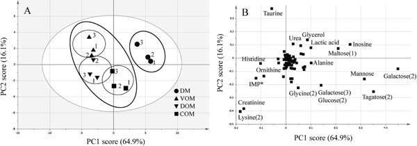
PCA of metabolic component profiles PCA was performed to identify trends and groupings in the data. In PCA based on the sample variance-covariance matrix, the first principal component (PC1) explained 64.9% and the second component (PC2) explained 16.1% of the total variation. A plot of PCA scores (Fig. 1A) visually distinguished samples based on metabolic components profiles, and a loading plot (Fig. 1B) identified constituents that contribute to differences among samples on the score plot. Fig. 1A shows clear separation based on PC1 between DM and OM samples. Additionally, samples of the OM group had moderate separation into three discrete groups. The loading plot shows the involvement of individual metabolic components contributing to the groupings shown in Fig. 1A. Looking at the loading of PC1, many metabolic components are located in the positive direction (i.e., sugars such as galactose). These metabolic components show a positive correlation with DM. On the other hand, the metabolic components to the left of the first principal component are correlated with VOM and DOM (i.e., lysine, creatinine, inosine monophosphate, ornithine, histidine, and taurine). PCA is a dimensional compression method having a minimum loss of multivariate information (Wallisch et al., 2014). Huang et al. (2011) used a colorimetric sensor array and PCA to evaluate the freshness of fish samples. Velioglu et al. (2015) used Raman spectroscopy and PCA to differentiate between fresh (never frozen) and frozen and thawed fish samples. In this study, PCA was used to assess the overall differences in metabolic component profiles among tissues. In particular, distinct differences were observed between OM and DM, and although the differences were slight, the three OM types could be distinguished.
Discriminant analysis with OPLS-DA OPLS-DA, a supervised classification method, was used to extract the systematic differences between known classes of samples with predictive and orthogonal variation (Bylesjo et al., 2006). In contrast to the results of the unsupervised PCA models, where the ability to distinguish among tissues originates only from the projection of variance, the class identity in OPLS-DA is given in a Y matrix to which semi-quantitative values are then correlated (Worley and Powers, 2013). In order to maximize the separation between metabolic components characterizing the DM and OMs, OPLS-DA was performed with pairwise comparisons for groups defined as having a discrete variable Y. The models for distinguishing between DM and OM in yellowtail were sufficiently separated by OPLS-DA based on metabolic components profiles consisting mainly of low molecular weight hydrophilic components (Fig. 2A). In this model, the number of model dimensions was 1+1+0. Models exhibited a reasonable separation between DM and OM and acceptable goodness of fit (R2Y = 0.992) and goodness of prediction (Q2Y = 0.953). R2 and Q2 values close to 1 mean a better fitting and more accurate model. In general, an R2 of 0.65 or more and Q2 of 0.5 or more indicate satisfactory quantitative predictive ability (Hotelling, 1933; Williams and Norris, 1987). The metabolic components that most contributed to class separation were selected by analyzing the correlation coefficient loading plot. The S-plots of the OPLS-DA models were used to identify potential markers of group separation as proposed by Wiklund et al. (2008). In the S-plot, the range of selected variables is highlighted with a dotted rectangle. Cut-off values were set as being greater than or equal to 0.05 and 0.5 for the absolute value of covariance p and correlation p(corr), respectively (Sieber et al., 2009), identifying 12 metabolic components as possible markers of tissue-specific constituents for separating DM and OM (Fig. 2B). Metabolic components showing a positive relationship with DM were alanine, galactose, glycerol, hypoxanthine, inosine, lactic acid, maltose, pantothenic acid and tagatose. On the other hand, metabolic components with a positive relationship with OM were creatinine, histidine, lysine and ornithine. Semi-quantitative values of the 12 metabolic components that can potentially distinguish DM and OM are shown in Table 2. A statistically significant difference was observed in the semi-quantitative values of DM and OM in metabolic components, except for lactic acid and tagatose. Notably, creatinine, inosine, lysine, maltose, ornithine and pantothenic acid showed marked differences with creatinine, lysine and ornithine present at high levels in OM, and inosine, maltose and pantothenic acid present at high levels in DM. Therefore, using these metabolic components as indicators may make it possible to distinguish OM and DM based on chemical composition.

Table 2.
Comparison of semi-quantitative values of candidate discriminant metabolites in dark muscle (DM) and ordinary muscle (OM)
| Metabolite |
Semi-quantitative value |
P value |
| DM |
OM |
| Alanine |
0.64 ± 0.06 |
0.36 ± 0.12 |
0.004* |
| Creatinine |
1.28 ± 0.06 |
3.21 ± 0.55 |
0.000004* |
| Galactose (2) |
7.92 ± 0.98 |
2.96 ± 1.84 |
0.0014* |
| Glycerol |
1.17 ± 0.06 |
0.67 ± 0.11 |
0.002* |
| Histidine |
0.34 ± 0.16 |
0.69 ± 0.16 |
0.008* |
| Hypoxanthine |
0.39 ± 0.02 |
0.18 ± 0.07 |
0.001* |
| Inosine |
3.41 ± 0.22 |
1.34 ± 0.32 |
0.000001* |
| Lactic acid |
1.81 ± 0.07 |
1.46 ± 0.26 |
0.05 |
| Lysine (2) |
0.64 ± 0.08 |
2.70 ± 0.64 |
0.000008* |
| Maltose (1) |
1.48 ± 0.16 |
0.21 ± 0.24 |
0.00003* |
| Maltose (2) |
0.31 ± 0.04 |
0.08 ± 0.05 |
0.004* |
| Ornithine |
0.11 ± 0.01 |
0.43 ± 0.11 |
0.00006* |
| Pantothenic acid |
0.15 ± 0.01 |
0.02 ± 0.01 |
0.00000001* |
| Tagatose (2) |
6.14 ± 1.58 |
3.42 ± 2.09 |
0.09 |
*
P < 0.05. * indicates significant differences by Student's
t test (
P < 0.05).
Numbers in parentheses after compound names are the same as in Fig. 1.
The component profiles of fish muscle are greatly affected by factors such as handling, storage methods and bacterial growth; therefore, markers for distinguishing tissues should be components that are not greatly affected by these factors. In this study, storage conditions were emulated for consumption as sashimi. Under the conditions adopted here, no significant changes were noted in bacterial growth and lipid oxidation in different tissue types of yellowtail (S. quinqueradiata) (Tanimoto et al., 2018). After death, ATP in fish is successively degraded to ADP, AMP, inosinic acid, inosine and hypoxanthine by a series of endogenous enzymatic reactions. The rates of degradation of ATP in the postmortem changes differ considerably in ordinary and dark muscle tissues (Murata and Sakahuchi, 1986). Consequently, hypoxanthine and inosine, which differ between muscle tissue types, are probably unsuitable as markers for distinguishing tissue types because they are likely to be affected by storage (Table 2). Free amino acids such as alanine, histidine, lysine and ornithine, as well as creatinine are reported to be present in higher levels in OM than DM (Sakaguchi and Murata, 1986). It has been reported that free amino acids are not greatly affected by cold storage (Murata et al., 1993) and, therefore, they could be candidates as effective markers for identifying tissue types. However, depending on the storage method, amino acids that are the constituents of protein, such as alanine, histidine and lysine, would likely be affected by proteolysis. On the other hand, there are no reports of changes in amino acids such as ornithine or pantothenic acid during storage, and these amino acids were selected as the dominant marker candidates, but future studies are needed to verify their stability during storage.
Next, the differences between tissue types of the OM were assessed using OPLS-DA score plots, and we found that it was possible to distinguish between tissue types of the OM (Fig. 3A). Each OM tissue type that did not show a large difference in PCA was clearly distinguishable. The first component (t[1]) separated COM from DOM and VOM. The second component (t[2]) separated DOM and VOM, though the difference was modest; and COM was located between VOM and DOM in t[2]. The first and second components explained 64.6% and 20.8% of R2X variation in metabolic patterns, respectively. In this model, the number of models was 2+0+0 (number of model dimensions), with 0.793 of R2Y and 0.68 of Q2Y. Thus, statistical analysis of metabolic components can make it possible to distinguish muscle tissue that is indistinguishable based on visual appearance. Discriminant metabolites are shown on S-plots (Fig. 3B, C). Fig. 3B is the S-plot for t[1]. Histidine and IMP are metabolic components showing the relationship between DOM and VOM. On the other hand, the other metabolic components shown in Fig. 3B show a relationship with COM. Fig. 3C is the S-plot for t[2]. Lactic acid and succinic acid are metabolic components related to VOM. On the other hand, metabolic components shown in Fig. 3C are metabolic components related to DOM. We further confirmed these through comparison of the peak area ratio between DOM, VOM and COM (Table 3). Significant differences were also confirmed by ANOVA of individual metabolic components that were shown to be important for distinguishing between the three groups. In particular, glycerol 3-phosphate, niacinamide and valine showed differences between the three tissue types.

Table 3.
Comparison of semi-quantitative values of discriminant metabolites in ordinary muscle (OM) tissue types
| Metabolite |
Semi-quantitative value |
ANOVA P values |
| Dorsal OM |
Ventral OM |
Caudal OM |
| Alanine |
0.34 ± 0.04ab |
0.25 ± 0.08a |
0.49 ± 0.07b |
0.012* |
| Asparagine |
0.07 ± 0.01a |
0.05 ± 0.00b |
0.08 ± 0.00a |
0.018* |
| Creatinine |
3.44 ± 0.10ab |
2.60 ± 0.54a |
3.58 ± 0.26b |
0.028* |
| Fructose-1-phosphate (1) |
nd |
0.03 ± 0.00 |
0.36 ± 0.17 |
0.025* |
| Fructose-1-phosphate (2) |
0.04 ± 0.02 |
nd |
0.39 ± 0.14 |
0.012* |
| Galactose (2) |
2.04 ± 0.88a |
1.65 ± 0.65a |
5.20 ± 0.99b |
0.004* |
| Glucose-6-phosphate (1) |
0.02a |
0.01a |
0.12 ± 0.01b |
0.003* |
| Glucuronic acid (2) |
0.18 ± 0.01 |
0.13 ± 0.01 |
nd |
0.002* |
| Glutamine |
0.04 ± 0.01ab |
0.02 ± 0.01a |
0.07 ± 0.02b |
0.014* |
| Glycerol-3-phosphate |
0.28 ± 0.05a |
0.14 ± 0.04b |
0.41 ± 0.01c |
0.0003* |
| Glycine (2) |
0.89 ± 0.21 |
0.55 |
1.08 ± 0.26 |
0.150 |
| Histidine |
0.82 ± 0.16 |
0.68 ± 0.15 |
0.55 ± 0.04 |
0.100 |
| Hypoxanthine |
0.26 ± 0.05a |
0.12 ± 0.02b |
0.15 ± 0.01ab |
0.024* |
| Inosine |
2.56 ± 0.81a |
0.87 ± 0.43a |
0.48 ± 0.20b |
0.001* |
| Inosine monophosphate |
1.20 ± 0.05a |
1.07 ± 0.11a |
1.74 ± 0.14b |
0.007* |
| Inositol |
0.17 ± 0.02a |
0.14 ± 0.02a |
0.25 ± 0.05b |
0.010* |
| Lactic acid |
1.21 ± 0.04 |
1.54 ± 0.17 |
1.63 ± 0.30 |
0.090 |
| Lysine (2) |
2.98 ± 0.59 |
2.13 ± 0.54 |
2.99 ± 0.53 |
0.171 |
| Maltose (1) |
0.17 |
0.04 ± 0.02 |
0.39 ± 0.27 |
0.19 |
| N-Acetylaspartic acid |
0.07 ± 0.01ab |
0.04 ± 0.02a |
0.08 ± 0.01b |
0.012* |
| N-Acetylmannosamine |
0.07 ± 0.01a |
0.06 ± 0.01a |
0.11 ± 0.02b |
0.013* |
| Niacinamide |
0.45 ± 0.03a |
0.31 ± 0.04b |
0.77 ± 0.04c |
0.00002* |
| Ornithine |
0.49 ± 0.15 |
0.38 ± 0.03 |
0.40 ± 0.08 |
0.508 |
| Phenylalanine |
0.28 ± 0.01a |
0.18 ± 0.03a |
0.50b |
0.004* |
| Phosphoric acid |
5.29 ± 0.58 |
4.57 ± 0.53 |
5.05 ± 0.42 |
0.292 |
| Serine |
0.06 ± 0.01 |
0.04 ± 0.02 |
0.09 ± 0.03 |
0.124 |
| Succinic acid |
0.11 ± 0.08 |
0.22 ± 0.29 |
nd |
0.053 |
| Tagatose (2) |
nd |
1.65 ± 0.65 |
5.20 ± 0.99 |
0.007* |
| Threonine |
0.29 ± 0.03ab |
0.20 ± 0.07a |
0.36 ± 0.05b |
0.024* |
| Valine |
0.20 ± 0.01a |
0.12 ± 0.03b |
0.25 ± 0.03c |
0.001* |
*
P < 0.05. Different lowercase letters on the same metabolite indicate significant differences by Tukey's test (P < 0.05).
Numbers in parentheses after compound names are the same as in Fig. 1.
nd = not detected
Glycerol-3-phosphate is an intermediate in triacyl glycerol and phospholipid synthesis (Lordan et al., 2017; Reshef et al., 2003). Niacinamide is a precursor of NAD+ and NADP+ through the salvage pathway. These coenzymes are essential for maintaining cellular redox homeostasis and for modulating numerous biological events, including cellular metabolism (Xiao et al., 2017). Valine is one of the branched chain amino acids. These amino acids are not only elemental components for building muscle tissue but also participate in increasing protein synthesis in animals and humans (Zhang et al., 2017). The semi-quantitative values of the above-mentioned three compounds were the highest and lowest in COM and VOM, respectively, potentially indicating that metabolism flows are different among the tissue types of OM depending on the function of the respective tissue type such as the motility. However, there have been no reports of metabolite composition by OM tissue type or changes during storage to date. Therefore, further investigation is needed to confirm that these three compounds are effective markers for distinguishing the three tissue types.
In conclusion, metabolic analysis clearly distinguished between DM and OM. The differences in metabolic profiles could be also be used to distinguish among three tissue types of OM. Further, metabolic components (ornithine for OM vs DM and glycerol-3-phosphate for OM tissue types) with various biochemical properties were important for differentiating among these muscle tissue types. In future, this strategy may be developed and utilized for other fish species.
Acknowledgements This work was supported by a grant from JSPS KAKENHI (Grant Number JP 26750023).