Original papers
Visualization of Browning Color Formation on Grilled Fish Through a 2D Simulation
2014 Volume 20 Issue 3 Pages 537-545
Details
2014 Volume 20 Issue 3 Pages 537-545
The aim of this work is to develop a 2D model for the effective visualization of browning color formation on the upper surface of a sample during far-infrared radiation heating. Temperature and color (CIE L*, a*, and b* values) at a central surface position on Japanese amberjack (Seriola quinqueradiata) and red sea bream (Pagrus major) were monitored over time. A mathematical approach was used to predict the upper surface temperature distribution according to the browning behavior of each sample by the insertion of noise functions. Estimated L*, a*, and b* values were obtained by inserting a plot of temperature profiles into the browning kinetic model. Color values were converted to an R′G′B′ color space, and the model was constructed using FEMAP software. The uniformity or non-uniformity of the browning color formation on the surface of the samples was visualized using the developed 2D model.
Color plays an important role in indicating how well food is cooked. Thus, if the changes in food color, such as the occurrence of browning during cooking, can be predicted and effectively modeled, cooking methods such as grilling can be improved.
In our previous works, the browning formation on fish during grilling was modeled according to the change in color intensity and did not directly involve chemical compounds. First, the browning of red sea bream was analyzed according to the relationships between color, sample surface temperature, and grilling time. A model that enables the prediction of fish surface color lightness (L*) from the surface temperature history was proposed. The values of a* and b* (fish surface color position on red/green and blue/yellow axes, respectively) were estimated from empirical equations obtained using near-infrared radiation (NIR) heating (Nakamura et al., 2011). Then, the browning of red sea bream grilled by far-infrared radiation (FIR) and superheated steam (SHS) heating, besides NIR heating, was analyzed. The results confirmed that the kinetic model developed in the previous work can be applied to the browning formation on fish during the grilling process, independent of the heat transfer mode (Matsuda et al., 2013). Then, the analysis of the differences in browning formation rate during grilling on the surface layer of several fish species, taking into consideration their intrinsic chemical composition, was conducted. As browning occurred, the color changes on the samples followed almost the same trajectory, except for salmon, which was probably due to its astaxanthin content. Samples with a higher fat content browned faster, in accordance with their higher browning rate frequency factor (k0) (Llave et al., 2014). Finally, the relationship between the progressive color changes during grilling and the progression of protein denaturation of the muscle, caused by the heat applied at the beginning of the grilling process, was analyzed. Surface color changes on fish during the beginning of grilling were estimated from the degree of protein thermal denaturation, obtained through differential scanning calorimetry (DSC) measurements. The total non-denaturation ratio using contributions of 0.70 and 0.30 from myosin and actin, respectively, was found to be the best fit for the changes in the L* values (Yu et al., 2014). In all cases, estimations were approximated to the measured colors, obtained by a colorimeter using the CIELAB color space. However, the fact that the measured data was collected from a single measurement point and that the all-round distribution of color on the surface was not evaluated raised the need for the present study.
Several authors, such as Hutchings et al. (2002), claimed that tristimulus colorimeters using the L*, a*, and b* color space are inherently unsuitable for assessing the color distribution and color uniformity measurements for many whole foods. These instruments only provide average values for small areas of the sample, and therefore, many locations must be measured to obtain a representative color profile (Mendoza et al., 2006). As a result, the measurements are not representative of heterogeneous materials such as most food items (Papadakis et al., 2000; Segnini et al., 1999), making the global analysis of the food’s surface more difficult (Mendoza and Aguilera, 2004; Papadakis et al., 2000; Segnini et al., 1999). Thus, these instruments can only provide average values, and it would be quite difficult and time-consuming if they were used for point-by-point measurements at many locations to obtain the color distribution (Yam and Papadakis, 2004). It is also difficult to obtain the whole color distribution when the color on the surface varies from point to point as a result of fat and moisture content, surface shape, and other factors. These drawbacks instigated our analysis of the color changes through an original simulation method based on one temperature measurement point at the center of the fish surface. Using a mathematical technique, the entire surface temperature distribution was estimated, and using our previously developed browning kinetic model, the all-over color of the upper surface was predicted. Finally, to appropriately visualize the browning color formation during grilling, a 2D model was built using FEMAP software (a modeling/finite element post-processing system). Therefore, the goal of this study was to develop a 2D computer-imaging model for visual simulation of the browning color formation on the upper surface of fish during FIR grilling. To deal with the different browning behavior of fish species and improve the browning visualization, mathematical noise functions were included to fine-tune corrections in the temperature distribution.
Materials Japanese amberjack (Seriola quinqueradiata) and red sea bream (Pagrus major) were used as samples in this study. These fish species were chosen because they are commonly used for grilling. They were purchased from a fish market on the day of the experiment, and in all cases they were under rigor mortis. The skin and bones were removed and the ordinary muscle of the fillets was cut into 3 × 4 × 1.5 cm samples for all experiments. The samples were wrapped in wrapping film and refrigerated at 5°C for no more than 30 min before use.
Experimental conditions Figure 1 shows a schematic diagram of the manually assembled laboratory-scale oven used in this study. The 12 × 12 cm FIR heater was a 100 V/750 W, electric ceramic plate heater (PLC-328) from Noritake Co., Aichi, Japan. The infrared energy radiated downward from the heater. The samples were positioned approximately 80 mm below the heat source on an electronic balance. The FIR heater was warmed up 30 min before starting the experiment and the radiation energy was measured three times during the grilling process. The FIR heater was adjusted to 420°C and the temperature at the sample point was confirmed to be 240 ± 1.8°C during the entire grilling process. The radiation energy, measured by a radiation sensor (RF30; Captec, Villeneuve d’Ascq, France) at the same sample position, was 2.8 × 10⁴ Wm−2 (with a standard deviation of 1.9%).
Surface temperature measurements The surface temperatures of the samples were measured using a K-type thermocouple (ø = 0.5 mm) at the center position. A single measurement profile was collected from each run using the sample with the longest grilling time. A personal computer, a data logger (Thermodac 5001A; Eto Denki Co., Tokyo, Japan), and software (Thermodac-E/Ef 2.6; Eto Denki Co.) were used to collect the temperature data. The accuracy of the surface temperature profiles collected using the K-type thermocouples was verified by comparing with profiles collected using IR sensors. For details, please refer to Matsuda et al. (2013).
Color measurements Changes in the color values on the fish surface were measured using the CIE L*, a*, and b* system at the same position as the surface temperature measurement was taken, using a spectrophotometric color difference meter (NF333; Nippon Denshoku Industries Co., Ltd., Tokyo, Japan). The L*, a*, and b* values were measured using a D65 light source with a viewing field angle of 2°. Sampling of the grilled fish was conducted at 0, 2, 4, 6, 8, and 10 min.
Construction of a 2D model for simulation of browning color To construct the 2D model, the steps presented in Fig. 2 were followed.
Construction of the surface temperature distribution The surface temperature profile of the center position was used to construct the whole surface temperature distribution using the following equation:
 |
Initially, the simulated browning color formation on the surface of the sample could not be visualized because the whole sample surface automatically received the same temperature from the beginning of the process. For this reason, a noise load (randomization) function was included on the surface of the model to simulate the heterogeneous temperature distribution behavior, observed particularly in low fat samples, such that normal random numbers generated by Excel, were incorporated into the surface temperature profile for each coordinate.

Experimental grilling apparatus of the FIR heater.

Steps followed to construct the 2D visualization browning color model.
To deal with the non-uniform browning of the sample surfaces, a noise (magnification) function was also used. To adjust the magnification function of the calculated surface temperature distribution, it was compared to the measured surface temperature distribution profile collected by an infrared (IR) thermographic camera (TH7102WV; NEC San-ei Instruments Ltd., Tokyo, Japan) with a resolution of 0.06°C (at 30°C) and an accuracy of ±2°C.
Thermographic analysis To adjust the calculated temperature distribution profiles, the fish sample surface temperature distribution was collected each minute using an IR thermographic camera, placed over the sample model at a 45° incline, with an emissivity value εj = 0.95. Thermographic images represent the spatial temperature distribution of surfaces based on measured infrared radiation (Tanaka et al., 2007). The IR thermographic camera was calibrated at surface temperatures ranging from 110 – 150°C by using calibrated optical fiber sensors. The surface temperature profiles were similar, with a variation of ± 0.6°C in the worst case. When comparing the whole profile, the mean of the absolute values of the relative error ( ) was 1.02%, with a standard deviation (SD
 ) of 0.43%. The method for evaluating the error was described in detail by Llave et al. (2012). This led to the conclusion that the surface temperature profile of the grilled fish could be determined accurately using the IR thermographic camera. From a total of 9,800 collected surface temperature data points, 1,200 data points nearest to the center of the sample surface were selected to avoid data points nearest to the external limits.
Calculation of the L*c, a*c, and b*c values The browning kinetics theory used in this study to determine the activation energies (Ea) and frequency factors (k0) of the reduction rate of the calculated L*c values of the samples was described in detail in our previous works (Matsuda et al., 2013; Nakamura et al., 2011). Using this theory, browning was modeled according to the color intensity change and did not directly involve chemical compounds. To determine the a*c, and b*c values, based on the L*c values, the empirical equations developed by Nakamura et al. (2011) were used:
 |
 |
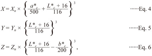
Conversion of the calculated color values from L*, a*, and b* to R'G'B' In order to analyze the color values by 2D computer simulation, it is necessary to convert the L*c, a*c, and b*c values of the CIELAB color space (hereafter called the L*c, a*c, and b*c values) into R′G′B′ values that can be better manipulated on a display color. Brosnan and Sun (2004) and Du and Sun (2004) explained the advantages of analyzing each pixel of the entire surface of the food and quantifying surface characteristics and defects by using R′G′B′ values. To perform the color system conversion, it is necessary to convert the data using three steps:
(1) L*c, a*c, and b*c to CIE XYZ
The L*c, a*c, and b*c values are based on the intermediate system CIE XYZ, which simulates human perception. Later, they are converted into RGB values. The following equations were used to convert L*c, a*c, and b*c into XYZ (Pascale, 2003):
For L* >8.0:
 |
(2) CIE XYZ to sRGB
To obtain the sRGB triads, the following three-by-three matrix transformations for the D65 illuminant and a 2° standard observer (Pascale, 2003; Wyszecki and Stiles, 1982) were performed using the recommended coefficients by the Rec. ITU-R BT.709–5 (2002), an International Telecommunication Union recommendation that defines the image format parameters and values for high-definition TV (HDTV); sRGB:
 |
After this operation, the sRGB coordinates of the illuminant were (100, 100, 100). All sRGB triads were rescaled at this point (divided by 100) and the illuminant coordinates became (1, 1, 1). Results greater than one or less than zero were clipped at one and zero respectively. Pascale (2003) claimed that for critical work, the series ITU-R BT.709 (sRGB) recommendations should be used if the images are to be distributed and viewed using unknown displays. Mendoza et al. (2006) also used the recommended ITU-R BT.709–5 coefficients in the opposite way, from sRGB to CIE XYZ. They claimed that the ITU-R BT.709 recommendation specifically describes the encoding transfer function for a video camera that, when viewed on a “standard” monitor, will produce excellent image quality.
(3) sRGB to R'G'B'
The sRGB values were transformed to the nonlinear R′G′B′ values using the following transformation method recommended by Pascale (2003):
 |
These equations are similar to those reported by Larraín et al. (2008) and Mendoza et al. (2006), who used Eq. (8) in the reverse manner; thus, they transformed R′G′B′ into sRGB.
In Eq. (8), the terms were added to scales and the values rounded to the nearest integer between zero and 255. This scale corresponds to 8 bits per primary, a 24-bit color system. For computer-generated images, a simple gamma (γ) correction is necessary for sRGB. This value is usually 0.45 (1/2.2) for sRGB, a space used only by Windows-based computers. In this way, R′G′B′, the gamma corrected coordinates, were obtained.
Construction of the 2D model The FEMAP software (10.2; NeiSoftware, CA, USA) was employed to construct the model, selecting the appropriate shape, size, and mesh of the sample. Although 3D images are presented below, the browning color formation was evaluated at the upper surface only, and therefore the analysis of browning was simulated in 2D only (X and Y axes). A sample model of a 4 × 3 × 1.5 cm slab shape was used for all experiments and is shown in Fig. 3. The X, Y and Z coordinates were divided using a mesh spacing of 5 mm, which results in an 8 × 6 × 3 mesh. The R′G′B′ color data were fed into the model, positioning the values at the meshes. We used workstations with a quad-core processor (CPU speed = 2.83 GHz, RAM = 4 GB), running the 64-bit Windows 7 Professional OS.

Sample model used in the computational modeling.

Temperature distribution on the upper surface of samples captured using an IR thermographic camera, in comparison to digital pictures after 6 min of FIR heating. A: Japanese amberjack, B: red sea bream.
Statistical evaluation Composition data were analyzed by oneway ANOVA, combined with Tukey’s pairwise comparison test, using the Systat statistical software (3.5; Systat Software Inc., IL, USA).
Surface color changes of fish samples The color of the fish surface at the center point during grilling was accurately determined by using the browning kinetic model (Llave et al., 2014; Matsuda et al., 2013; Nakamura et al., 2011). In this study, the calculated color and b*c for both species were found to be in good agreement with the respective measured values (not shown). Therefore, if L*c declines, a*c and b*c change accordingly; although it was also observed that the heating rate accelerates or decelerates the color changes. Hosseinpour et al. (2013) reported that for color changes in shrimp during drying, a decreased L* could be attributed to non-enzymatic browning, brown pigment formation, and lipid oxidation resulting from the classic Maillard reaction between carbonyl and free amino groups, as well as carotenoid destruction and astaxanthin degradation. Additionally, Contreras et al. (2008) claimed that it might also be related to an increase in the samples’ opacity, resulting from structural shrinkage due to moisture evaporation.
The accuracy of the model was observed even for species that present a large difference in fat content (the fat content for Japanese amberjack and red sea bream is 13.8% and 2.0%, respectively). Llave et al. (2014) reported the intrinsic behavior of browning color formation for some fish samples according to their chemical composition. In the case of Japanese amberjack, a uniform surface color formation was found, in contrast with that of red sea bream, which presents a non-uniform brown color formation. Similar results were found here. Figure 4 (A-B) shows the results after 6 min of FIR heating for Japanese amberjack and red sea bream, respectively, captured using an IR thermographic camera, along with digital pictures from the same time step. Figure 6 shows changes in color during grilling at several time points.
Estimation of the surface temperature distribution The upper surface temperature distribution profile for Japanese amberjack and red sea bream were estimated from a single collected temperature profile, as explained above, at all time points. Next, the temperature distribution was modified and adjusted for the special behavior of each fish sample by customizing using an α function for fine tuning. Figure 4 (A-B) shows a higher and more homogeneous increment of surface temperature for the Japanese amberjack sample compared to the red sea bream sample under the same conditions. The mathematical correction procedure conducted in this study made it possible to obtain a similar temperature distribution profile as the upper surface temperature distribution profile collected by the use of the IR thermographic camera.

Comparison of the whole surface temperature distribution profiles measured by the IR thermographic camera and calculated using Eq. (1) after 6 min of FIR heating. A: Japanese amberjack, B: red sea bream.
These results are shown in Fig. 5 (A-B) for Japanese amberjack and red sea bream, respectively. The best agreement of the profiles with a lower relative error () was obtained for α values of 0.06 and 0.11 as the mean values for Japanese amberjack and red sea bream, respectively. The mean absolute () value between the profiles was 0.33%, with a standard deviation (SD) of 0.063%, a of 5.7% and a SD of 0.12% for Japanese amberjack and red sea bream, respectively. For more details on the error determination, refer to Llave et al. (2012).
The results showed a normal distribution for the surface temperature distribution on Japanese amberjack, with a frequency temperature in the range of 180 – 230°C and a peak temperature of 200°C. This contrasts with the distribution on red sea bream, which had a wider frequency temperature, in the range of 130 – 240°C, and a smaller peak temperature at 180°C. These differences justified the use of the magnification function in Eq. (1) to deal with the different intrinsic behavior of the fish species that show changes in local temperatures due to the shrinkage phenomenon, as explained by Braeckman et al. (2009) and Llave et al. (2014).
| Kinetic Parameters | Japanese amberjack | Red sea Bream |
|---|---|---|
| *Ea [kJ mol−1] | 49.6 ± 0.2a | 50.7 ± 0.2a |
| *k0 [s−1] | 9875 ± 62.2a | 4759 ± 51.9b |
Ea: activation energy; k0: frequency factor; *Mean ± standard deviation of the kinetic parameter values (n = 3); values with different superscripts within a line are significantly different ( p < 0.05).
Moreover, randomization of the surface temperature profiles by the Ra function was necessary to deal with the temperature equilibrium behavior observed on the upper surface after several minutes of simulated heating. Since the thermographic technique is a fast online method of analyzing temperature distribution, providing a full thermal landscape (Björk et al., 2010), its utilization in future color analysis during grilling is desirable.
Estimation of the surface color distribution The previously obtained temperature distribution at any position on the upper surface was used to calculated the L*, a*, and b* color values using the browning kinetic model, to obtain the color profiles at the same positions. Different color patterns were observed among these profiles. More specifically, for red sea bream, a low fat species, a non-uniform browning color formation was observed on the fish surface. Llave et al. (2014) analyzed the kinetic results of the reduction rate of L*c values of the fish species during the grilling process. Their results for the fish species considered in this study are presented in Table 1 for discussion. The frequency factors (k0) of both species had significantly different values (p < 0.05). This may be due to their different crude fat content. The results show that the higher the fat content, the higher the reduction rate of L*c value. This is reasonable because the browning color for samples with a high fat content, such as Japanese amberjack, is more intense than for those with a low fat content (see Fig. 6).
Fish grilling causes a mass transfer of water from the surface by evaporation, due to the elevated temperatures used during the process. This dynamic process changes the flat surface to a curved surface, a phenomenon known as the shrinkage effect, and thus the initial flat surface topography (obtained in sample preparation) may not remain homogeneous. The irregular undulations on the surface not only disturb the direction and distribution of the reflected light intensities but also produce shadows on the surface having varied temperatures (Mendoza et al., 2006).
Thermal processing causes the release of free water in muscle, which then evaporates and causes a further decrease in surface moisture levels of the product; this drying is influenced by the initial moisture content of the sample. Decreasing the moisture content decreases the color lightness of the sample, whereas other color parameters are increased (Hosseinpour et al., 2013). Similar results were obtained in this study. For example, in the case of red sea bream, the moisture content values were 0.75, 0.74, 0.72, 0.72, 0.72, and 0.70 (kg/kg-muscle) for the entire sample, whereas values for the surface position obtained from the external 1 mm of the crust portion were 0.75, 0.71, 0.66, 0.63, 0.56, and 0.43 (kg/kg-muscle) at 0, 2, 4, 6, 8, and 10 min, respectively. Moreover, the moisture reduction during grilling was less intense for Japanese amberjack than for red sea bream, probably due to its lower initial moisture content (0.64 kg/kg-muscle). For details of the moisture content determination, please refer to Llave et al. (2014). These browning characteristics of grilled samples, strongly dependent on the moisture content, are relevant when constructing a model.

Comparison of photographs and images of browning color formation of red sea bream and Japanese amberjack simulated in X and Y axes using FEMAP software.
Simulation of browning color by a 2D visualization model L*c, a*c, and b*c values were converted into R′G′B′ values using the equations presented above. Then, to construct the visualization model, the R′G′B′ values were plotted into the FEMAP software.
Figure 6 shows the comparison of photographs and the simulated browning color formation on Japanese amberjack and red sea bream at several time points. All considered cases had temperatures above 100°C to avoid the effect of protein denaturation, as was described in detail by Yu et al. (2014). Samples with similar sizes and weights were used in the experiment. The surface temperature was measured and photographs were taken at nearly constant time intervals. The results show a good approximation of the model to the photographs at any sampling period. To relate the browning color formation visualized by the model to the photographs (known as color matching), a final assessment was conducted on the color pattern of the inscription to deal with the color change range observed during browning reaction by the simulation. These color changes are recognized from a very pale white color at the beginning of the browning process (just after the protein denaturation reaction is finished), changing to an obscure brown color at the end of the browning formation and at the same time as the start of the carbonization reaction. For this purpose, the final color range using R′G′B′ values, obtained as a consequence of the color transformation, were inserted into the FEMAP software. Thus, the default color range of the inscription was modified for better visualization of the color reproduction. This final adjustment of the color reproduction is a necessary step (Valous et al., 2009) that is usually followed by image analysis using a computer vision system (CVS). Several authors (Brosnan and Sun, 2004; Du and Sun, 2004; Hutchings et al., 2002; Larraín et al., 2008; Leon et al., 2006; Mendoza and Aguilera, 2004; Mendoza et al., 2006; Valous et al., 2009) have reported that CVS can be an efficient tool for determining the color of food surfaces. However, in order to objectively measure color and to accurately detect color features in food products using CVS, color characterization, as well as evaluation of the reproducibility of the camera’s sensor, are essential steps in the implementation of any CVS, as color information captured by digital cameras is device-dependent (Valous et al., 2009). Moreover, in the case of bio-processing, as in the present study, the complexity becomes more pronounced because of the heterogeneity of biological materials, which indicates different exclusive characteristics under processing activities, even under the same operating conditions (Nazghelichi et al., 2011). These problems are overcome by the method described in this study.
The differences in the uniformity of the surface color described above were satisfactorily simulated by the developed 2D model. These results are in agreement with the results presented in Fig. 5, in which Japanese amberjack exhibited a higher and more homogeneous surface temperature distribution than red sea bream. After 6 min of grilling, black spots were observed on the upper surface of the red sea bream as a result of the carbonization reaction, and it was concluded that this was a consequence of the highest temperature existing at these positions. Therefore, the white spots observed at the same time represent positions of the lowest temperature.
Because the CIELAB color space is recognized as the most appropriate for representation of surfaces or materials with natural curvatures and undulations (Mendoza et al., 2006), its use, combined with the browning kinetic model in the present study, improved the prediction accuracy of the 2D model. Hosseinpour et al. (2013) and Leon et al. (2006) claimed that the L*, a*, and b* color space gives a more uniform distribution of color and their results match human perception more closely. Similar results were found here. Moreover, the conversion into R′G′B′ values permits better manipulation of the data by computer simulation of the upper surface color, resulting in a good approximation to the photographs. Thus, differences in browning formation explained by differences in the chemical composition of the fish species were visualized independent of their typical uniform or non-uniform surface distribution of brown color.
Effective visualization of the browning color formation on grilled fish is a necessary challenge in line with the demand for enhanced food quality. The present study focused on the development of a computer 2D imaging model to simulate the browning color formation on fish surfaces during grilling. The model used R’G’B’ values obtained from L*, a*, and b* values, by a sequential mathematical transformation through intermediate color spaces. These L*, a*, and b* values were previously predicted from the browning kinetics model based on a single measurement of surface temperature profile at the center position during grilling. An empirical equation was used to estimate the temperature distribution of the entire upper surface. To deal with the different browning behavior of fish species, due to differences in chemical composition, and improve the browning visualization, mathematical noise functions were included to fine-tune corrections in the temperature distribution. Finally, the FEMAP software was used to build a 2D model and simulate the browning color formation as temperature increases during grilling. We reached the following conclusions:
A single temperature profile from the center of the upper surface of the samples can be used to accurately simulate the entire upper surface color distribution by the appropriate use of the mathematical technique explained here.
The randomization and magnification noise functions of the temperature distribution of the upper surface sample can be treated accurately through the simulation of browning color formation of fish species, even though they present a typically uniform or non-uniform browning behavior.
Transformation of L*, a*, and b* values to R'G'B' color coordinates permits an accurate and reliable simulation of the browning formation on fish samples during grilling.
The black spots observed on the surface of some fish species, as a result of water evaporation as well as the impact of the shrinkage phenomenon during the grilling process, were appropriately simulated using the 2D model developed in this study.
Acknowledgements This work was supported in part by a Grant-in-Aid for Scientific Research (C) from the Ministry of Education, Culture, Sports, Science and Technology of Japan (22500728).