Original Research Papers
Population Balance Model for Crushed Ore Agglomeration for Heap Leach Operations
2014 Volume 31 Pages 200-213
Details
2014 Volume 31 Pages 200-213
Agglomerate size distribution is a pretreatment step in low grade heap leach operations. The present work focuses on modeling the evolution of size distribution in batch agglomeration drum. Up to now there has been no successful work on modeling of crushed ore agglomeration although the framework for population balance modeling of pelletization and granulation is readily available. Different batch agglomeration drums were used to study the agglomeration kinetics of copper, gold and nickel ores. The agglomerate size distribution is inherently subject to random fluctuation due to the very nature of the process. Yet, with careful experimentation and size analysis the evolution of size distribution can be followed. The population balance model employing the random coalescence model with a constant rate kernel is shown to work well in a lab scale agglomerator experiments. It was observed that in a small drum agglomerates begin to break in a short time whereas the growth is uniform in the larger drum. The experimental agglomerate size distributions exhibit self-preserving size spectra which confirms the applicability of coalescence rate based model. The present work lays out the fundamentals for applying the population balance concept to batch agglomeration, specifically crushed ore agglomeration. The experimental difficulties and how to overcome them are described.
Heap leaching is one of the promising economic and green processes for the treatment of lean ores of copper, nickel, and gold. Acid or cyanide solution is percolated through a large heap of ore body and leached out metal is collected after several days.
During heap building i.e. the transport of ore material to the heap, severe segregation of material can occur which results in poor bulk permeability and ore percolation. Introduction of agglomeration step prior to heap building results in minimal segregation and solution flow through heap. It is well understood that percolation is highly dependent on the size distribution of the crushed ore, because fine particles tend to wash out and plug the pores in the heap. Therefore, it is important to bind fines to coarse particles to improve overall percolation.
Agglomeration pretreatment is required for ores which either contain excessive amounts of clay or an excessive quantity of fines generated during crushing. While agglomeration has become common pretreatment step in heap leach operations, the fundamental understanding of the agglomeration process for crushed ores is still lacking (Bouffard, 2005; Dhawan et al., 2013).
Crushed ore agglomerates can take two forms: fine particles adhering to coarse particles and fine particles adhering to each other. The former is similar to granulation whereas latter is referred as pelletization. For binder assisted agglomeration, adhesion and cohesion forces are dominant whereas surface tension and capillary forces prevail in non-binder/wet agglomeration (Kodali et al., 2011).
The residence time for agglomeration and the binding agents dominantly control the growth and mechanism of agglomeration. For hard to crush ores, the dominant mechanism of agglomeration growth is layering of fines on bigger particles, i.e., rim agglomerates whereas, newly nucleated agglomerates are expected to be more prevalent in high clay content ores such as nickel-laterite ores.
Generally, the agglomerated ore has a distinct particle size distribution (PSD) with a slight increase of the top size but a very large increase in the lower sizes. Typically, sizes are 60 mm to 2 mm with all of the minus 2 mm adhering to the coarser particles or between themselves (Miller, 2010). The author reviewed the crushed ore agglomeration process up to 2012 and did not come up on modeling studies on the topic (Dhawan, 2013; Dhawan et al., 2013). Some of the possible reasons can be the stochastic nature of process, experimental difficulties and lack of instrumentation for fundamental studies. Therefore, in this work the fundamentals for applying the population balance concept to batch agglomeration is laid out. Also, some other aspects of the evolution of agglomerate size distribution (ASD) are carefully studied using four different ores.
Agglomeration results from direct interactions between discrete particles, and the agglomerate formation and growth can be mechanistically described with phenomenological models (Hogg, 1992). The basic mechanisms observed in agglomeration systems include coalescence, crushing and layering, snowballing and nucleation. These have been discussed in detail in the past (Kapur and Fuerstenau, 1969, Sastry, 1975; Kapur and Runkana, 2003; Liu et al., 2012).
Coalescence refers to the production of large-size agglomerates by clumping or fusing together of two or more particles. When agglomerates collide and stick or pack together in a geometric configuration favorable with respect to the rest of the moving charge, the conglomerate of agglomerates begins to roll and eventually deforms and forms the next larger agglomerate. The coalescence events cause discrete changes in the size of the agglomerates with an overall decrease in the agglomerate population without any change in their mass. Often coalescence is observed to be the most important mechanism responsible for growth in a batch system. Coalescence mechanism contributes wholly or partially to the growth of agglomerates made from materials of wide size distributions, whereas crushing and layering mechanism is the dominant mode in narrow sized particle populations (Kapur and Fuerstenau, 1969; Sastry, 1975; Kapur and Runkana, 2003). These authors reported that it holds strongly in the initial stages of agglomeration and almost throughout the batch agglomeration of materials with naturally comminuted and wider size distributions. Coalescence applies to wide distributions due to size independence, whereas crushing and layering applies to narrow size distributions due to size dependence. Unlike pelletization, the crushed ore agglomeration primarily contains wider feed size distribution of sizes up to 1.5 inch, employs retention times as low as 1–3 min and lacks stable acid-binder within the bed. Moreover, the coexistence of fines (minus 75 micron) micron and larger sizes makes the growth mechanism and particle-particle interaction cumbersome in agglomeration.
At present no definitive modeling studies have been reported on crushed ore agglomeration (Dhawan et al., 2013). Considering these facts, modeling studies of pelletization and granulation forms the starting point. In the past, pelletization and granulation have been studied in detail. The pelletization studies were carried out with very fine sizes in the 100 μm size range whereas granulation studies were also restricted to a maximum feed size of 10 mm. In these studies, it is important to mention that narrow feed size distribution, longer agglomeration times and stable binder conditions were the influencing factors. The size enlargement modeling has been done primarily with the concept of population balance model. Pelletization systems have utilized the coalescence model, whereas granulation studies used partition coefficient for an equilibrium model without considering agglomeration kinetics (Litster et al., 1986; Kapur and Runkana, 2003).
The population balance for a well-mixed batch system undergoing coalescence alone is described in the literature (Kapur and Fuerstenau, 1969; Kapur and Runkana, 2003) as Eq. (1).
| (1) |
In this equation, u and v refers to volume of agglomerate, n(v, t) is the number density function, λ(u, v, t) is coalescence kernel rate, NT is the total number of particles at time t, and α is space system parameter. This is the time continuous and size continuous population balance model.
The total volume should be conserved in the system since agglomerates of volume vi and vj combine together to form an agglomerate of volume vi + vj at all times as shown in Fig. 1.

Schematic of coalescence mechanism.
In modeling, coalescence is the most difficult mechanism. However, it is needed to formulate the population balance in terms of number distribution by volume because granule volume is conserved in a coalescence event. An important parameter in population balance modeling (PBM) is the growth rate (coalescence kernel (λ)) that signifies the degree of agglomeration. The kernel dictates the overall rate of coalescence, as well as the effect of granule size on coalescence rate. The order of the kernel has a major effect on the shape and evolution of the granule size distribution. Most of the kernels are empirical or semi-empirical and must be fitted to plant or laboratory data. Modeling growth where deformation is significant is more difficult. It can be assumed that a critical cutoff size determines which combination of agglomerate sizes is capable of coalescence. Coalescence of particles is mainly dictated by its inertia. As with chemical reactors, the degree of mixing within the agglomerator has an important effect on the final ASD because of its influence on the residence time distribution (Snow et al., 2009).
Four ores provided by different mining companies were used in this study. The ores were screened into various size fractions and the size distribution of ores used in the experiments is shown in Fig. 2. The major difference between the ores is weight percentages of minus 200 mesh. Copper ore-II and nickel ore feeds are finer than gold ore and copper ore-I (minus 200 mesh% Cu-I: 7.4, Cu-II: 23.6, Au: 10.6, Ni: 14.9). The top size fed to the laboratory agglomerator was limited to 13 mm to insure that agglomerates were not too large for subsequent column leaching and secondly to accommodate the size and capacity of the drums used in this study. The bulk densities of copper-I, copper-II, nickel and gold ores are 1.42, 1.55, 1.17 and 1.67 g/cc, and the natural moisture content is 0.26, 2.6, 13.4 and 1.4%, respectively.

Feed size distributions of different ores used.
The preliminary experiments were conducted using a micro-agglomerator as shown in Fig. 3. The agglomeration drum was made using a 1 liter fluorinated polyethylene (FLPE) Nalgene bottle 9 cm in diameter by 17 cm in length. Three polytetrafluoroethylene (PTFE) lifters placed 120° apart were attached in the drum. Each lifter was 2 cm wide, 14.3 cm long and 6 mm thick. The small drum was mounted in a horizontal bracket and was driven with a 24 V D.C. motor and can run at variable speeds up to 76 rpm (Dhawan, 2013).

Image of micro-agglomerator and ancillary equipment.
Based on several experiments, it was observed that in small drums the presence of large particles hindered the growth of other agglomerates. This caused incomplete agglomeration and thereby failing the objective of studying the behavior of each ore type. To avoid such behavior, lab-scale drum, shown in Fig. 4, was used in this study. This drum is a copy of the drum used in previous studies by Kapur and Fuerstenau (1969) and Sastry and Fuerstenau (1973) at the University of California Berkeley. The drum is a fully enclosed water-tight drum machined from an aluminum block, measuring 12 inches in diameter and 6.9 inches in length. Twelve lifters of 20 mm diameter were attached length wise uniformly around the inner periphery of the drum to prevent any sliding of the charge and imparted a rolling and cascading action to the agglomerates. The inner surface of the drum was lined consistently with silicone coated polyurethane gloss finish to eliminate ore charge sticking. The drum lining was refurbished whenever there was a change in ore type. The use of scraper was not considered to avoid any interference with the experiment. A transparent acrylic plastic cover on the drum enabled convenient withdrawal of product and observation of the charge motion.

Photograph of the agglomeration drum.
In crushed ore agglomeration, volume loading is generally kept low, up to 8%. This low volume filling of the drum can be seen as a single layer of charge and thereby not enough capacity to carry on. In general, large particles migrate to the outer side of cascading charge, whereas smaller particles are at the lower or inner region. Under these conditions large particles can break intermediate size agglomerates.
For PBM, number size distribution is a prerequisite. Therefore, batch experiments corresponding to different time intervals were conducted in the lab-scale drum. Following the experiment, number size distribution for each time step was also determined in an image analysis set up. A batch of known weight corresponding to 7% volume loading was introduced into the drum. Next, the drum was rotated for 5 min without any other additives. Then a premeasured amounts of sulfuric acid solution (Copper ore-I, II and nickel ore) or cyanide solution (gold ore) was added to the drum in a short time (less than 30 seconds). In other words, the ore was prewetted to minimize the incomplete wetting of the tumbling charge during solution delivery.
After that, the drum was closed with the lid and was placed on two horizontal rubber rollers. It was rotated at 24 rpm (30% critical speed) for a specified time. At a predetermined time interval, the rotation was stopped and the moist agglomerated ore was spread on a tarp. The material was further sampled by cone and quartering technique a representative sample of 450–500 grams was collected. The sample was air dried at room temperature for 24 hours. Then the dried sample was analyzed under image analysis set up for number size distribution. To avoid experimental error or concerns regarding effect of drying and sampling, for each time interval, a new batch experiment was conducted for the entire duration of 1, 2, 2.5, 3 or 4 min.
The standard cone and quartering technique was used in this work only because there are no other practical methods that will work with soggy ore agglomerates that have a wide size distribution. The material is piled in a heap so that the natural segregation in the heap is nearly symmetrical. The conical pile is then spread from the center to form a flattened disk of material. Then, the disk is divided into quarters using a flat wooden plank. A pair of opposite quarters is removed, and the other pair is used as the representative sample. Depending on the mass needed, the material can be coned and quartered again. Certainly, the procedure is tedious, time consuming and prone to human error. The representative agglomerate sample was air dried at room temperature before sieve size analysis.
The procedure for number size distribution of agglomerates involves primarily image analysis and shape factor to convert between mass and number distribution. A dry sample was placed on black paper under the image analysis setup. Individual agglomerates particles were moved apart from each other on the paper so that there was no overlap. The setup requires proper lighting conditions so that the particles do not reflect light. The pictures were taken by a camera (Fujifilm® FINEPIX® XP10). Next, the images were processed through ImageJ® software from which the number size distribution was obtained. Once the particles are captured in an image file, each particle area is known and its size is determined. In the image analysis, it is assumed that the particles are spherical in shape. This may be a very drastic assumption but very much necessary for modeling. In the modeling part the volumes of particles are added to generate agglomerate volume. Considering the different response of each ore type, the shape factors effect was not included in the population balance model. However, using shape factors, converting number size distribution (image analysis) to weight size distribution (sieve size) is possible.
The time evolution of the PSD is commonly obtained from the solution of the general population balance model governing the dynamic behavior of a particulate process. Several numerical methods have been used for solving the steady-state or dynamic population balance equation. These include the full discretization method (Hounslow et al., 1988), method of moments, fixed and moving pivot discretized methods (Sastry and Gaschignard, 1981), high-order discretized methods (Ramkrishna and Mahoney, 2002). Based on the detailed literature review, the PBM equation used in this work was adapted from Kapur and Runkana (2003).
The rate of coalescence in restricted-in-space environment should be proportional to number of particles of size i and number fraction of particles of size j, or vice versa. Hence, specific rate constant or coalescence kernel λ by definition is independent of the size of the interacting agglomerates. Under these stipulations, the generalized PBM Eq. (1) reduces to Eq. (2) (Kapur and Fuerstenau, 1969; Sastry and Fuerstenau, 1973; Kapur 1978).
| (2) |
The basic postulate of the model is that the particle mass is well mixed and the collision of frequency and the probability of coalescence are independent of size. The coalescence model also assumes that the nucleation of the moist feed has already been completed in the first few revolutions and hence, only the mechanism of coalescence is operative.
In this model, the size interval is discretized into a large number of intervals. Interval i represents a volume vi of particles in that interval. Further, interval i is assumed to represent a volume i × v1 where v1 is the smallest volume representing the first interval. Such a formulation allows a pair of size classes to coalesce and yet form a larger volume that is already defined as a size class. Thus, volume conservation is guaranteed. In the model Eq. (2), ni(t) is the number of particles of size i at time t in the agglomeration drum, λ is average random coalescence rate constant, N(t) is total number of particles at time t. The derivative term in the Eq. (2) gives the time rate of number of particles of size i. The second term depicts the disappearance of size i due to agglomeration of size i with all other sizes. The third term depicts that the formation of particles of size i due to coalescence (below size i) of size i with size i-j.
In this formulation, particle of size i disappear in proportion to the number fraction nj(t)/N(t) of particles of size j surrounding it. Likewise, particles of size i agglomerate with size j in proportion for the number fraction of size i surrounding it. Summing Eq. (2) over all sizes, it can be shown that the rate of depletion of the total number of agglomerates, N(t), conforms to the first order decay kinetics as shown in Eq. (3). The solution of Eq. (3), which is the total number of agglomerates at any instant N(t) is given by Eq. (4).
| (3) |
| (4) |
However, the random coalescence model includes some assumptions. It involves pure agglomeration process; all agglomerates are spherical and equal probability of coalescence for all size classes. It can be argued that a single-parameter coalescence kernel is sufficient for short agglomeration time provided the total volume of the system is conserved. If necessary, the single coalescence kernel can be transformed into a matrix form. In other words, the coalescence between size class i with class j can be distinguished with a coalescence rate λij instead of a single value of λ used for all size classes. Under this formulation, Eq. (2) is rewritten as Eq. (5). Therefore, the coalescence kernel becomes a set of m2 values or m × m matrix, where m is the total number of intervals. The kernel matrix is symmetric because rate of coalescence is identical for size i with size j as it is for size j with size i.
The matrix enables the assignment of coalescence rate values as is needed between particles. However, this assignment is done from a primary value λ determined. For example, two large particles of sizes 20 and 24 mm cannot coalesce to form 44 mm agglomerate. Hence, their coalescence rate may be set to a small value, small as λ/100. The lambda matrix can predict size distribution more accurately if the precise interaction between sizes can be formulated.
| (5) |
The matrix formulation is shown in Fig. 5. The coalescence rate λ is determined graphically by plotting the total number of agglomerates remaining as a function of time. The analytical solution to the integro-differential equation is only known for special forms of the coalescence kernel with an assumed initial number density distribution.

Formulation of Lambda matrix for random coalescence model.
The lack of analytical solutions necessitates the use of numerical techniques. A popular method is method of size discretization (Kapur and Runkana, 2003) that involves discretizing the particle size domain into a relatively small number of size classes, and then monitoring the number and mass of particles in each size class so as to minimize if not eliminate the finite domain error. Volume is used as the size descriptor for the sake of convenience in handling death and birth terms. Often in the laboratory, the size distribution is measured with a set of sieves. Since a few sieves are used, only size fractions are measured in each size interval. In other words, the measured information is not sufficient to convert to the continuous density function. Therefore, the reverse course is followed: discretize the continuous size model, and get a discretized model with discrete solution.
As per model Eq. (2), the volume intervals and number of particles in each volume interval were specified. Assuming all agglomerates as perfect spheres and knowing their respective size fractions were the prerequisites for the model framework. Considering the maximum agglomerate size to be approximately 25 mm that covers a volume of 10,000 mm3, 4,000 intervals each of volume 2.5 mm3 were used to cover the entire volume range. For example, 1.7 mm agglomerate means agglomerate retained on 1.7 mm screen and passed through 2.5 mm screen.
Similarly, the number size distribution of particles at time zero or particle size distribution of the drum feed was also calculated. Based on the volume intervals, a set of 4,000 ordinary differential equations (ODE’s) were solved simultaneously using Matlab software. After each experiment the number of agglomerates with their respective sizes was determined. A MATLABTM code was written to count the number of agglomerates in each volume interval. The population balance model was solved using discretization procedure at defined screen sizes. The numerical package used for solving the set of differential equations was the Matlab function “ode45 and ode15s”, which is an ODE solver within the “Optimization” toolbox. Both of the functions were yielding very similar results. Since ode45 function was taking less time, it was selected for all the simulation work. The ode45 solver uses a variable step Runge-Kutta numerical algorithm. For all the simulations, a time step of 0.001 min was used.
The experiments were determined based on the numerous preliminary experiments done in the lab-scale and micro-agglomerator drums. The results of these experiments were also used for determining optimum agglomeration conditions. However, for the sake of brevity only typical results are shown here. Preliminary experiments were conducted on copper ore using fine feed size distribution (minus 1 mm) to test the applicability of the population balance model. For modeling purposes, one expects a gradual and smooth coarsening of size distribution. The evolution of PSD with time should be smooth as it is in other size enlargement operations.
From image analysis methodology, it was observed that the number of agglomerates remaining in the drum is decreasing with increase in residence time. The coalescence rate was different for each experiment and also varies with the amount of solution added. The range of coalescence rate for all the experiments is 0.4–2.4 per minute. A typical model prediction as compared to experiment results is shown in Fig. 6. It is evident that model prediction and experimental results are in agreement.

Comparison of experimental number size distribution and model predictions for fine copper-I ore feed at different time.
Based on the success of PBM model predictions in fine feed experiments, scoping experiments were performed in the microagglomerator with wide feed size distribution. Fig. 7 show typical copper ore model predicted and experimental agglomerate size distribution. It is evident from the figure that model prediction and experimental results are not satisfactory. Moreover, there is not a smooth transition of ASD with time as was expected. In fact, ASD corresponding to 3 and 6 min are same, which indicates saturation or equilibrium size distribution.

Comparison of experimental number size distribution and model predictions for coarse copper-I ore at different time.
Based on many similar experiments, it was confirmed that longer retention times lead to restricted growth or finer ASD which indicates there is breakage of agglomerates. In particular, the majority of the experimental ASD showed breakage after 3 min. Since ASD curves collapse on each other it seems that after certain time there is an equilibrium size distribution. It can be argued that breakage and agglomeration occurs in the drum within 3 min. Therefore, in this study, larger retention time was not attempted because most plant scale agglomerators run at 2 or 3 min mean retention time. The expectation is that in the first 3 min growth is much larger than breakage.
In regular crushed agglomeration, however, the evolution of PSD with time is not as smooth as it is in other size enlargement operations such as pelletization. The sources of such behavior include, (1) irregular shape of agglomerates which makes it difficult to determine actual volume, (2) mixing of ore particles with acid solution seems to be never uniform within the agglomerator unless prewetted, (3) agglomerates break mainly due to weak adhesion between large and small particles, (4) due to lack of wetting of fine ore particles, the growth rates may vary in the small and intermediate sizes, (5) in general, small particles layer large particles, but if too much fines are present, they themselves, can agglomerate but they break up on collision. In the first few revolutions, the nucleation of the moist feed completes, but due to lack of uniform wetting nucleation itself is random.
The modeling of agglomeration with PBM is approached with a view to make it reasonably simple so that it may become a tool in plant operations for the prediction of ASD. However, the inevitable irregularities in the experiments pose a severe challenge to the approach. Obviously, agglomerates are not perfectly spherical and wetting with acid solution is not uniform either. However, with these considerations, it is worthwhile to see how crushed ore agglomeration may be brought under control to study the underlying growth rates.
It was thought that the reason for some of the unfavorable model predictions is due to the use of single coalescence rate for all size classes. The logical next step is to try different coalescence rate for pairs of size classes, i.e., the coalescence rate constant is different pairs of coalescing size classes, as described in model Eq. (5).
The cumulative number fraction passing using a single lambda value (scalar lambda), experimental data and a matrix of lambda values is compared in Fig. 8. It is quite clear that experimental data do not fit really well with different matrix lambda for most of the ASD. Rather, the model prediction fits well with the single value of lambda. However, with a better understanding of coalescence rate of different sizes, the matrix predictions can be improved. However, the matrix formulation requires more detailed micro-scale investigation of underlying mechanisms that was beyond the scope of this work.

Comparison of experiment and and model predictions at t= 3 min for copper-I ore using lambda matrix.
Coalescence rate model worked well even with an approximated growth rate. The prediction for first few minutes was accurate however it fails at longer retention time because the size distribution does not conform to regular growth behavior for any ore. With these experimental and model analyses, it was realized that the experiments should be done in a larger drum. It was expected that due to more free space in a larger drum, better cascading action and regular growth will occur. Therefore, to study the agglomeration behavior of different ore types and to delineate the other relevant effects all modeling experiments were done in the lab-scale drum.
Although no rigorous statistical analysis of the experimental precision has been attempted, it is nevertheless important to consider in a qualitative sense the possible source of errors. The two main sources of error are the procedure adopted for measurement of the agglomerate size and the stochastic nature of the process. Firstly, the agglomerates are not geometrically perfect spheres and the measured agglomerate size is based on the estimate of circular diameter. Moreover, the image analysis system loses its precision at sizes less than 1 mm. The second error is due to stochastic fluctuations of size distribution about the average agglomerate size mean. Agglomeration dynamics is subject to probabilistic laws, and as such, two agglomeration experiments carried out under identical conditions have only a finite probability of showing the same ASD.
In the small agglomeration drum, however, the stochastic nature is magnified due to small number of agglomerates participating in each size class. In very large drums the stochastic nature will be smoothed out by the very large number of agglomerates present.
Based on preliminary experiments it was evident that higher retention time (i.e., more than 3–4 min) does not contribute to further agglomerate growth. Therefore, the maximum retention time in the drum was limited to 4 min. Since the coalescence rate plays a major role in the underlying model, its accuracy is vital. Hence, all experiments were done at four time intervals so that better approximation of slope can be obtained. To avoid experimental errors such as stopping the drum to collect the sample, each time step was done in different batches. Therefore, one complete experiment involves four batch experiments between 1–3 min. Each experiment was carried out at different moisture conditions and was part of the planned agglomeration growth range. Also, the drum volume filling (7%) and drum speed (30% Nc) were kept constant for all experiments.
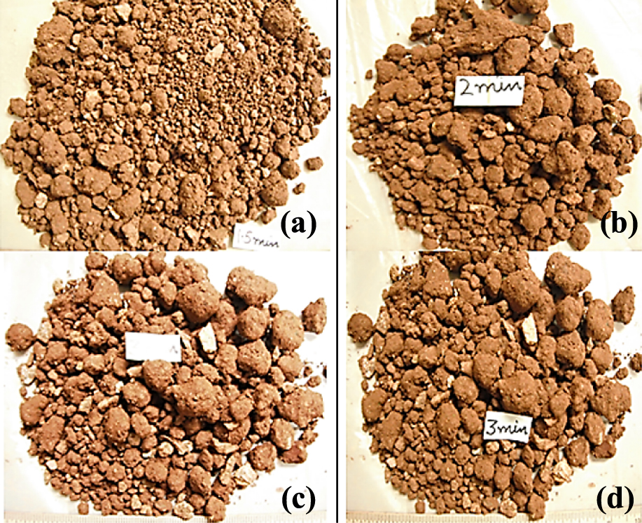
The visual appearance of agglomerates is one of the first hand experiences regarding agglomeration behavior. Long duration agglomerates are generally characterized by smoother surface and shape. A typical screen shot of copper-II ore agglomerates under image analysis set up is shown in Fig. 9. It is evident from the figure that agglomerate shape becomes more regular (spherical) at a longer retention time.

Typical screenshot of copper-I ore agglomerate samples under image analysis set up at different time intervals (increasing left to right: (a) 1.5 min, (b) 2 min, (c) 3 min, (d) 4 min.
A series of experiments were done with copper-I ore in the lab scale drum. A typical experiment results is shown here. Fig. 10, 11, 12 show the photographs of the agglomerates, experimental ASD, semi-log plot of total number versus time, and model prediction overlaid on experimental data. It is difficult to recognize any appreciable growth pattern from agglomerate photographs. But the surface sheen increases at high moisture conditions as seen in Fig. 10.

Photograph of copper-I ore agglomerate sample at different time intervals (increasing left to right: (a) 1.5 min, (b) 2 min, (c) 3 min, (d) 4 min.

Agglomerate size distribution for copper-I ore (weight percent).

Semi-log population plot for growth rate determination for copper-I ore.

Comparison of experimental number size distribution and model predictions for copper-I ore at different time intervals.
In each of these experiments some overlap between successive ASD was noticed as in Fig. 11(a). The growth rate was not large enough to show sufficient advance in these intervals. The closeness or cluster between ASD curves possibly indicates that certain equilibrium size distribution is unique for agglomerates and it will not move further irrespective of retention time. In some experiments it is evident that the model prediction for initial time, i.e., 1 min does not fit well with experimental ASD. This is due to the slope approximation made from 0–4 min (Fig. 11b). It can be seen from the population plot that the number of agglomerates decreases at a faster rate during the initial 1 min period than other times. This is due to the presence of a large amount of fines present at start time. In other words, the decay or population of agglomerates is not progressing at exactly same rate as expected in the model. Even then, with average growth rate, the model predictions are still satisfactory as shown in Fig. 12. Similar results were obtained for different experiments involving different moisture content. Similarly, copper-I ore experiments were also conducted in the micro-agglomerator in order to study the variation in growth rates in different size of drums.
Fig. 13 compares the growth rate as a function of moisture between the microagglomerator and the lab-scale drum. The growth rate trend is the same in both the drums. However, the coalescence rate was slightly less in microagglomerator as compared to the lab-scale drum. Obviously, there is better cascading and tumbling action achieved in the lab scale drum and hence the higher growth rate. Moreover, the breakage problem arises at longer agglomeration times in the microagglomerator. Considering the similar behavior of agglomerates in these two drums, all experiments for nickel, gold and copper-II ores were only done in the lab-scale drum.

Comparison of variation of coalescence rate with moisture for copper-I ore.
Similarly series of experiments were done with nickel laterite ore, copper-II and gold ore at different moisture levels in the lab scale drum. For the nickel ore, based on the photos as shown in Fig. 14, there is a notable absence of surface sheen on the agglomerates even at high moisture content (36%). However, long duration agglomerates were possessing smoother surface and shape. It was observed that moist ore sticking was slightly higher at longer time for this ore; therefore, agglomeration time was limited only to 3 minutes.
Photograph of nickel ore agglomerate sample at different time intervals, increasing left to right: (a) 1.5 min, (b) 2 min, (c) 2.5 min, (d) 3 min.
The population decay or decrease in the number of agglomerates with time was more uniform. On drying, agglomerates became highly friable and hence released a significant amount of fines on contact. Hence, the size measurement was restricted up to 2 mm for the same reason. It is important to mention that the background color of image analysis setup was changed to light grey to gain contrast between agglomerates and background.
The gradual growth of agglomerate under specified conditions points to a good fit between experiments and model prediction. The ASD at different time intervals were plotted in accordance with the random coalescence model. A comparison of experimental and predicted ASD is shown in Fig. 15. It can be seen that there is a reasonable fit between experiment and the model prediction. The closeness between experimental data and the theoretical lines confirms the soundness of the model.

Comparison of experimental number size distribution and model predictions for nickel ore at different time intervals.
It can be observed from Fig. 16 that moisture content certainly alters the coalescence or growth rate. However, for most of the experiments it is close to 1.1 min−1, which is slightly less than that for copper-I ore. For practical purposes, an average value of coalescence rate 1.1 min−1 is reasonable for nickel ore.

Variation of coalescence rate (λ) with moisture content for nickel ore.
For copper-II ore, there is slight difference in visual appearance among different experiments. The slight difference between appearances is the dark contrast at high moisture conditions. A surface sheen was never observed on this ore type even at high moisture content, because of high clay content. However, long duration agglomerates had a smoother surface and regular shape as shown in Fig. 17. Based on scoping experimental results, the agglomeration times were confined up to 3 min. It is important to mention that the population decay or decrease in the number of agglomerates with agglomeration time was steepest for copper-II ore as compared to copper-I ore and nickel laterite ore. The agglomerates were of different characteristics in terms of shape and partial wetting.

Photograph of copper-II ore agglomerate sample at different time intervals, increasing left to right: (a) 1 min, (b) 1.5 min, (c) 2 min, (d) 3 min.
From experimental observations, it was seen that as soon as the liquid was added to the charge, lumps were formed. Therefore, some particles were found unwetted even after agglomeration. It was rare to observe any remaining fine particles for copper-II ore. Since there is appreciable agglomerate growth under specified conditions, it is reasonable to expect a good fit between experiments and model prediction. The ASD at different time intervals were plotted in accordance with the random coalescence model as shown in Fig. 18. There is some misfit between experimental and predicted ASD. This is because of steep slope change from 0–1 min as compared to other times. Also, the absence of intermediate size classes in this ore type leads to unusual agglomeration behavior.

Comparison of experimental number size distribution and model predictions for copper-II ore at different time intervals.
The value of coalescence rate is almost twice as compared to copper-I and nickel laterite ore as shown in Fig. 19. In general, there seems to be a midpoint value close to 14% moisture where the rate is at its maximum value. However, for most of the experiments it is close to 1.9 min−1, which is almost twice that for nickel ore. For practical purposes, an average value of 1.9 min−1 is useful.

Variation of coalescence rate with moisture for copper-II ore.
Unlike other ores, the photographs of gold ore agglomerates at different time intervals and at different moisture conditions show a significant variation. With each time step, the transition to smoother surface and shape, appearance of coarser agglomerates at longer times are evident as shown in Fig. 20. The appearance of surface sheen on the agglomerates indicates the range of optimum moisture content. Considering the regular agglomerate growth shown by agglomerates under specified conditions, it is reasonable to expect a regular fit between experiments and model prediction. A comparison of experimental and predicted ASD is shown in Fig. 21. It can be seen from these figures that there is reasonable fit experiment and model prediction. The closeness between experimental data and the theoretical lines confirms the soundness of the model.

Photograph of gold ore agglomerate sample at different time intervals (increasing left to right: (a) 1 min, (b) 1.5 min, (c) 2 min, (d) 3 min.

Comparison of experimental number size distribution and model predictions of gold ore at different time intervals.
The growth rate of gold ore under different moisture conditions is shown in Fig. 22. In general, there seems to be a midpoint value close to 7–8% moisture where the growth rate is maximum. However, for most of the experiments it is close to 1.2 min−1, which is nearly the same as that of copper-I ore and nickel ore.

Variation of coalescence rate (λ) with moisture for gold ore.
For comparison purposes, the variation of coalescence rate with moisture for all ore types is shown in Fig. 23. For each ore type, the moisture content certainly changes the growth rate. In general, there seems to be an optimum moisture value where maximum rate was observed. However, based on magnitude copper-II ore grows almost at a rate two times as that of nickel ore.

Variation of coalescence rate for all ore types with moisture.
In general, it can be seen that the overall agreement is reasonably good between experimental size distributions and those predicted by the random coalescence model. Considerable deviation occurs, especially at the initial time step due to rapid coalescence of fines in the feed. In some experiments the number size distribution curves overlapped at two different times. This is expected in view of the fact that, firstly, the coalescence rate constant used in the development of this model was taken to be a constant for all agglomerate sizes, and secondly, any error in the measurement of the circular diameter of the agglomerate is magnified on taking its cube when computing the agglomerate volume.
Sastry (1975) reported that agglomerate growth by coalescence is a sufficient condition for observing the self-preserving size spectra, which implies that there exists a unique ASD in a batch system which is independent of the material and processing conditions. The similarity distribution of the agglomerates is independent of the ore type and conditions of agglomeration, and is uniquely determined by the coalescence kernel.
It has been reported that the pellet growth by coalescence is a sufficient condition for observing the self-preserving size spectra and not necessarily the only one. Also, self-preserving size spectra of green pellets is a characteristic of the batch agglomeration. Mathematical analysis of the coalescence process indicated that there exists a self-preserving, pseudo-time-independent size distribution of agglomerates.
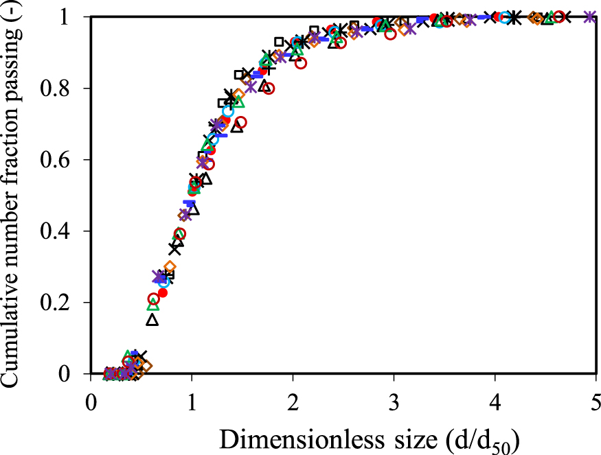
Based on mathematical transformations, it was argued if the coalescence kernel is a homogeneous function of its arguments, then the coalescence process has a self-preserving type of size distribution. However, it was emphasized that such a self-preserving distribution may be only a particular solution and may or may not be unique (Sastry, 1975). In other words, when experimental data exhibits self-preserving spectra then random coalescence is a valid approach to pursue. Therefore, the numerical solution of the population balance model with constant coalescence rate and experimental data for gold ore is plotted in Fig. 24.

Experimental self-preserving agglomerate number size distribution for gold ore.
Computed self-preserving agglomerate number size distribution for gold ore.
Population balance model for batch agglomeration has been developed. The model predicts the evolution of ASD in the batch agglomeration drum. The size distributions of the agglomerates in the specified time are adequately described by the random coalescence model. The model was verified for four ore types and different moisture level for each ore type. The kinetics of agglomeration designated by the coalescence rate is affected by the moisture content of the system. The copper-II ore exhibits the highest growth rate, whereas nickel laterite ore exhibits the slowest rate among the ores tested. A reasonable fit implies that the model accurately accounts for agglomerates growth due to coalescence taking place in the drum. The population balance model is more than adequate for application to batch agglomeration drums. The use of small drums leads to both agglomeration and breakage within a few minutes. The use of larger drums smooth out random fluctuations and minimizes breakage of agglomerates. Hence, for modeling purposes the use of as large drum as possible is recommended. Agglomerates are certainly irregular particles. However, the assumption of spherical agglomerates held pretty well in the population balance modeling effort. Experimental ASD exhibit self-preserving spectra and is found to be independent of operating conditions and is uniquely determined by the coalescence mechanism.
The authors would like to thank AMIRA International and the sponsors (related mining companies) for permission to publish the work. The authors also acknowledge the funding from AMIRA under P986 project. Any findings, opinions, and conclusions in this paper are those of the authors and not those of AMIRA International or its sponsors. Thanks are due to Professor Michael Moats, Michael Free and JD Miller for active discussions throughout the work.
Nikhil Dhawan
;%0A%09%09%09newWindow.document.open();%0A%09%09%09newWindow.document.write('<img src=%22./Graphics/31_2014011_25.jpg%22>');%0A%09%09%09newWindow.document.close();%0A%09%09)
Nikhil Dhawan did his B.Tech in Metallurgical Engineering at Punjab Engineering College, India. Afterwards, he received his Ph.D. in Metallurgical Engineering at the University of Utah, USA under supervision of Prof. Raj Rajamani. His research interest includes comminution particularly HPGR technology and agglomeration practice. Presently he is working as a scientist at CSIR-IMMT Bhubaneswar, India.
Samira Rashidi
;%0A%09%09%09newWindow.document.open();%0A%09%09%09newWindow.document.write('<img src=%22./Graphics/31_2014011_26.jpg%22>');%0A%09%09%09newWindow.document.close();%0A%09%09)
Samira Rashidi is a Ph.D. student in Metallurgical Engineering. She received her BSc and MSc degrees from AmirKabir University, Iran. Her Ph.D. thesis is mainly about studying energy-size relationships of different ores in lab-scale HPGR. Her background research focuses on modelling and simulation of comminution technology.
Raj Rajamani
;%0A%09%09%09newWindow.document.open();%0A%09%09%09newWindow.document.write('<img src=%22./Graphics/31_2014011_27.jpg%22>');%0A%09%09%09newWindow.document.close();%0A%09%09)
Raj Rajamani is a professor of Metallurgical Engineering Department at the University of Utah. His research interests are: Modeling charge motion in ball, SAG and AG mills, fluid flow in pulp lifters, CFD modeling of hydrocyclones, modeling of high pressure grinding rolls and eddy current separation of electronic waste. He is recipient of Gaudin Award (2008) for his work in the application of DEM methods in the modeling of charge motion in grinding mills and for his contributions to the basic science of comminution and classification. He received his B.E. (Honours) degree from Annamalai University, India, M. Tech from Indian Institute of Technology, Kanpur, India and Ph.D. from the University of Utah.